Tau Neutrinos Underground: Signals of $\nu_{\mu}\rightarrow\nu_{\tau}$ Oscillations with Extragalactic Neutrinos

Abstract

The appearance of high energy tau neutrinos due to $\nu_{\mu}\rightarrow\nu_{\tau}$ oscillations of extragalactic neutrinos can be observed by measuring the neutrino induced upward hadronic and electromagnetic showers and upward muons. We evaluate quantitatively the tau neutrino regeneration in the Earth for a variety of extragalactic neutrino fluxes. Charged-current interactions of the upward tau neutrinos below and in the detector, and the subsequent tau decay create muons or hadronic and electromagnetic showers. The background for these events are muon neutrino and electron neutrino charged-current and neutral-current interactions, where in addition to extragalactic neutrinos, we consider atmospheric neutrinos. We find significant signal to background ratios for the hadronic/electromagnetic showers with energies above 10 TeV to 100 TeV initiated by the extragalactic neutrinos. We show that the tau neutrinos from point sources also have the potential for discovery above a 1 TeV threshold. A kilometer-size neutrino telescope has a very good chance of detecting the appearance of tau neutrinos when both muon and hadronic/electromagnetic showers are detected.

I Introduction

A recent breakthrough in the study of neutrino oscillations came from the observation by the Super-Kamiokande experiment of a deficit of upward-going atmospheric muon neutrinos [1]. The observed electron neutrino flux was found to be consistent with the theoretical expectation from models of cosmic ray production of neutrinos. Furthermore, SuperK measurements are consistent with earlier experiments [2, 3, 4, 5] which detected anomalous ratios of the $\nu_{\mu}$ to $\nu_{e}$ flux. The new high-statistics data disfavor scenarios in which $\nu_{\mu}$’s oscillate into sterile neutrinos ($\nu_{s}$) [6], and the data are consistent with $\nu_{\mu}$ to $\nu_{\tau}$ oscillation (99$\%$ CL) with a large mixing angle, $\sin^{2}\theta>0.84$ and a neutrino mass squared difference of $2\times 10^{-3}$ eV${}^{2}<\Delta m^{2}<6\times 10^{-3}$ eV².

Direct detection of $\nu_{\tau}$ appearance is extremely difficult because at low energies, the charged-current cross section for producing a tau is small and the tau has a very short lifetime. Several long-baseline experiments with accelerator sources of $\nu_{\mu}$ [7, 8, 9, 10, 11] have been proposed with the goal of detecting tau neutrinos from oscillations, thus confirming the SuperK results. The only convincing evidence of neutrino oscillations to date involves astrophysical sources, neutrinos from the sun and atmospheric neutrinos. These observations involve indirect measurements, namely the disappearance of the expected neutrino fluxes.

We have recently discussed the possibility of using a kilometer-size neutrino telescope to detect tau neutrinos from extragalactic sources of high-energy neutrinos such as Active Galactic Nuclei (AGN) and Gamma Ray Bursts (GRB), assuming $\nu_{\mu}\leftrightarrow\nu_{\tau}$ with the oscillation parameters of the SuperK experiment [12]. The probability for $\nu_{\mu}\rightarrow\nu_{\tau}$ is given by [13]

$$P(\nu_{\mu}\rightarrow\nu_{\tau};L)=\rm{sin^{2}}2\theta\,\,\,\rm{sin{{}^{2}}}\Biggl{(}\frac{1.27\Delta m^{2}({\rm eV}^{2})L({\rm km})}{E({\rm GeV})}\Biggr{)}\,.$$ (1)

Assuming two flavor oscillations, muon neutrinos produced in AGN or GRB would oscillate to tau neutrinos as they travel to the Earth. Over astronomical distances in the range of a megaparsec to thousands of megaparsecs, by measuring tau neutrino fluxes, one could, in principle, probe oscillations down to $\Delta m^{2}\sim 10^{-17}$ eV², nine orders of magnitude below current neutrino experiments [14, 15]. On the other hand, for the SuperK parameter range, with $\Delta m^{2}$ on the order of $10^{-3}$ eV² and $\sin^{2}2\theta\simeq 1$, the oscillation probability is 0.5. It is this latter possibility that we explore in this paper.

We use the simplest assumption for the flavor content of extragalactic sources of neutrinos, in the absence of oscillations, for the ratio $\nu_{e}:\nu_{\mu}:\nu_{\tau}$ to be $1:2:0$. This is based on a counting argument applied to $\pi\rightarrow\mu\nu_{\mu}$ and $\mu\rightarrow\nu_{\mu}e\nu_{e}$ processes. With the two-flavor oscillations suggested by the SuperK experiment, the flavor ratio becomes $1:1:1$ after the neutrinos have traveled over astronomical distances. Even in the three-flavor oscillation scenario, the ratio is still $1:1:1$, because the path length of high energy extragalactic neutrinos is much larger than any neutrino oscillation length supported by the solar, atmospheric or accelerator data [16].

The ratio for $\nu_{e}:\nu_{\mu}$ might get modified at high energies due to muon cooling [17]. In addition, $\nu_{e}$ from neutron decay might give significant contribution, resulting in neutrino fluxes dominated by electron neutrinos as in the case of diffuse neutrino fluxes from propagating cosmic rays [18]. We comment qualitatively in the discussion section on how our results are altered with more realistic, flavor-dependent neutrino energy cutoffs. Regardless of the flavor content of the source, the maximal mixing suggested by the SuperK experimental results mean that there will be an appreciable tau neutrino component at the Earth, so one is interested in tau neutrino detection in high energy neutrino telescopes such as ANTARES [19], NESTOR [20], AMANDA [21] and the next generation of large underground detectors [22].

Tau neutrino detection requires an understanding of the effect of propagating through the Earth on the tau neutrino flux. The propagation of ultra-high energy tau neutrinos through the Earth is quite different from muon and electron neutrinos. The Earth never becomes opaque to tau neutrinos, while muon and electron neutrinos are absorbed via charged-current interactions before reaching the opposite surface [14]. Ultrahigh-energy tau neutrinos interact in the Earth producing taus which, due to the short lifetime, decay back into tau neutrinos with lower energy. This cascade continues until the tau neutrinos reach the detector on the opposite side of the Earth or until the energy of the neutrinos is small enough that the interaction length of the neutrino is longer than the path length through the Earth. The energy and nadir angle dependence of the extragalactic tau neutrinos fluxes have been examined quantitatively in Refs. [12, 23]. For certain fluxes, those that do not decrease too steeply with energy, there are significant enhancements of the tau neutrino flux relative to the muon neutrino flux at energies below $\sim 10^{6}$ GeV.

An enhancement of the tau neutrino flux does not necessarily translate to dramatic modifications of the standard model (no-oscillation) rates for upward-going muons, especially in view of uncertainties in the normalization of the extragalactic fluxes. However, by comparing rates for upward-going muons with rates for upward hadronic/electromagnetic (EM) showers, the signature of tau neutrino interactions is unambiguous for a large range of neutrino fluxes. In the next section, we briefly introduce the extragalactic and generic $\nu_{\tau}$ fluxes $F_{\nu_{\tau}}^{o}\sim E^{-n}$ for $n=1,2$ that are used here. After reviewing neutrino propagation through the Earth, we describe $\nu_{\tau}$ signatures. The fluxes considered here have a range of energy behaviors. Even if the normalizations of the neutrino fluxes are uncertain, and in some cases optimistic, it is useful to make quantitative comparisons of the event rates for upward muons and upward hadronic/EM showers, with and without neutrino oscillations, which we do in Section IV. The quantitative results for specific models lead to model independent conclusions, which we summarize graphically. Tau neutrino appearance would provide an independent confirmation of the SuperK results and would point towards the better understanding of physics beyond the Standard Model.

II High Energy Neutrinos Sources

Active Galactic Nuclei are the most luminous objects in the Universe. Most of this radiation comes from their central region, indicating that the energy radiation most likely comes from accretion of matter into a superheavy black hole. Protons within the AGN may get accelerated via first order Fermi acceleration to very high energies. They interact with protons and photons in the infalling gas, or they may exist in the jets along the rotation axis and interact with photons there. Photon-proton and proton-proton interactions produce pions, which decay into charged leptons, neutrinos and photons. Energetic photons ($E_{\gamma}\sim 100$ MeV) from about 40 AGN observed by the EGRET collaboration [24], and TeV photons have been detected from Mkn 421, Mkn 501 [25] and 1ES2344+514 [26]. Although these photons are conventionally explained by inverse Compton scattering from energetic electrons, this explanation is not without problems, and a hadronic origin of gamma-ray photons from AGN is a viable alternative [27]. If a large fraction of the observed energy in high energy photons from AGN is produced in hadronic interactions, then AGN are also powerful sources of ultrahigh-energy (UHE) neutrinos [28, 29, 30, 31].

In Fig. 1 we show neutrino fluxes predicted in the AGN models of Stecker and Salamon [28] and Mannheim Model A [29]. Both of these models predict neutrinos fluxes that represent the upper bounds for their class of the models. In particular, the Stecker-Salamon flux is an upper bound for AGN core emission, while Mannheim Model A is an upper bound for AGN jet emission models. Stecker-Salamon flux is bound by the the diffuse X-ray background, while Mannheim flux is bound by the extragalactic gamma ray background. The steep, low energy neutrino flux in Mannheim’s model is the emission from the host galaxy via $pp$ interactions of the AGN protons in the galactic gas disk. Since this part of the flux is derived with the assumption that all protons end up in the disk, it should be regarded as an upper bound. Stecker-Salamon flux at energies above 1 PeV may get reduced due to the cooling of pions and muons in the strong magnetic fields of AGN cores [17]. The fluxes plotted in Fig. 1 are for the sum of muon neutrino plus antineutrino, at the source, namely, without accounting for oscillation over astronomical distances. We label the fluxes in the absence of oscillations by $F^{s}_{\nu+\bar{\nu}}$.

Another extragalactic source with powerful radiation and possibly associated high energy neutrino flux are the gamma ray bursts (GRB). Several models have been proposed in order to explain the origin of GRB’s [32, 33]. In the fireball model [33], the gamma ray bursts are produced by the dissipation of the kinetic energy of the relativistic expanding fireball with a large fraction, $>10\%$, of the fireball energy being converted by photopion production to high energy neutrinos [34]. Photomeson production takes place when extremely energetic protons accelerated at high energies in the ultra-relativistic shocks interact with synchrotron photons inside the fireball. The decay of these charged pions and subsequently produced muons then produce electron and muon neutrinos. Contributions from proton-proton collision can be neglected in this model. In Fig. 1 we show the neutrino fluxes for gamma ray burst model of Waxman and Bahcall (GRB_WB)[35], in which they parameterize the flux by

$$F^{s}_{\nu+\bar{\nu}}(E)=4.0\times 10^{-\alpha}E^{-n},$$ (2)

where $\alpha=13$ and $n=1$ for $E<10^{5}$ GeV and $\alpha=8$, $n=2$ for $10^{5}<E<10^{7}$ GeV and $\alpha=1$, $n=3$ for $E>10^{7}$ GeV.

Theoretical work has been done to set upper bounds on high energy neutrino fluxes from AGN jets and GRB [35]. The bounds are based on the theoretical correlations between the cosmic ray flux and/or the extragalactic gamma ray flux and the neutrino flux. These bounds have some model dependence, and they tend to be weaker in the range of energies considered here than at higher energies ($E\sim 10^{7}-10^{9}$ GeV). The AGN and GRB neutrino fluxes used here satisfy these bounds.

Cosmic topological defects (TD) such as magnetic monopoles, cosmic strings and domain walls are predicted to be formed in the Early Universe as a result of symmetry breaking and phase transition in Grand Unified Theories (GUTs) of particle interactions. In the TD models, $\gamma$-rays, electrons (positrons), and neutrinos are produced directly at ultra-high energies via cascades initiated by the decay of a supermassive elementary “X” particle associated with some Grand Unified Theory, rather than being produced in high energy hadronic interactions. The X particle is usually thought to be released from topological monopoles left over from GUT phase transition. It decays into quarks, gluons, leptons. In this paper, we consider neutrino fluxes from topological defects models of Sigl-Lee-Schramm-Coppi (TD_SLSC) [36] and the model of Wichoski-MacGibbon-Brandenberger (TD_WMB) [37]. The main difference between these two models is the main channel for energy loss of the string network, in the former it is the gravitational radiation, while in the later it is the particle production. Both of these fluxes should be regarded as upper limits for TD models, because they have been constructed in such a way to satisfy the bound imposed by the measured cosmic ray and gamma ray fluxes [38]. These fluxes are shown in Fig. 1, where we take representative flux of WMB model with the string mass parameter giving the largest neutrino flux that is consistent with cosmic ray data. This flux is also below the Frejus [39] and Fly’s Eye [40] experimental limits on the neutrino flux.

We also consider two generic fluxes that have a power law behavior. The flux

$$F^{s}_{\nu+\bar{\nu}}(E)=10^{-7}{(E/{\rm GeV})^{-2}}(\rm{cm}^{-2}\rm{s}^{-1}\rm{sr}^{-1}\rm{GeV}^{-1})\$$ (3)

gives numerically stable results, however, our calculations with a flux with $F^{s}\sim E^{-1}$ is unstable at very high energies. Consequently, we use

$$F^{s}_{\nu+\bar{\nu}}(E)=10^{-13}{(E/{\rm GeV})^{-1}}{1\over(1+E/10^{8}{\rm GeV})^{2}}\ (\rm{cm}^{-2}\rm{s}^{-1}\rm{sr}^{-1}\rm{GeV}^{-1})$$ (4)

as a way to cutoff the high energy behavior. We show results for attenuated fluxes for neutrino energies up to $10^{6}$ GeV. We have chosen the multiplicative factors in $E^{-1}$ and $E^{-2}$ fluxes in such a way that they exceed atmospheric flux at neutrino energies between 10 TeV and 100 TeV. The upper bound for strong source evolution discussed recently by Waxman and Bahcall [35] would correspond to a limit of $2\times 10^{-8}E^{-2}$ (in the same units as Eq. (2)), a factor of 5 smaller than the choice of normalization we take in this paper.

We also show in Fig. 1 the atmospheric neutrino flux at zenith angle of $0^{\circ}$ and the horizontal flux. In our evaluation of the atmospheric backgrounds, we use the atmospheric muon and electron neutrino fluxes as a function of zenith angle [41].

We do not consider the neutrino flux from cosmic ray interactions with the microwave background. This diffuse neutrino flux is typically present at energies higher than we consider here [42], and it gives low event rates [30]. Furthermore, the cosmic ray interactions with the solar atmosphere are another source of neutrinos, however, for energies above a TeV, the flux scales as $E^{-3}$ or steeper [43]. As we see below, tau neutrino regeneration will not be a very important feature in fluxes with such large spectral indices.

III Tau Neutrino Propagation through the Earth

For neutrino energies above 1 TeV, the oscillation probability for $\nu_{\mu}\rightarrow\nu_{\tau}$ in the Earth is less than a percent for the parameters constrained by the SuperK experiment. As a consequence, we can neglect neutrino oscillation in our evaluation of tau neutrino propagation accounting for interactions in the Earth.

The coupled transport equations for the fluxes of the tau neutrino and its charged partner are given by

$$\frac{\partial F_{\nu_{\tau}}(E,X)}{\partial X}=-\frac{F_{\nu_{\tau}}(E,X)}{\lambda_{\nu_{\tau}}(E)}+\int_{E}^{\infty}dE_{y}G_{\nu_{\tau}\rightarrow\nu_{\tau}}(E_{y},E,X)$$ (5)

$$+\int_{E}^{\infty}dE_{y}G_{\tau\rightarrow\nu_{\tau}}(E_{y},E,X)$$ (6)

and for taus as,

$$\frac{\partial F_{\tau}(E,X)}{\partial X}=-\frac{F_{\tau}(E,X)}{\lambda_{\tau}(E)}-\frac{F_{\tau}(E,X)}{\lambda_{\tau}^{dec}(E,X,\theta)}$$ (7)

$$+\int_{E}^{\infty}dE_{y}G_{\tau\rightarrow\tau}(E_{y},E,X)+\int_{E}^{\infty}dE_{y}G_{\nu_{\tau}\rightarrow\tau}(E_{y},E,X).$$ (8)

Here $F_{\nu_{\tau}}(E,X)$ and $F_{\tau}(E,X)$ are differential energy spectrum of tau neutrinos and tau respectively, for lepton energy $E$, at a column depth $X$ in the medium defined by

$$X=\int_{0}^{L}\rho(L^{\prime})dL^{\prime}.$$ (9)

The density of the medium a distance $L$ from the Earth-atmosphere boundary, measured along the neutrino beam path, is $\rho(L)$. The lepton interaction length (in g/cm²) is $\lambda(E)$ and $\lambda_{\tau}^{dec}(E,X,\theta)$ is the decay length of the tau.

The functions $G_{i\rightarrow j}$ schematically represent interaction or decay contributions to lepton $j$ from lepton $i$. We limit our evaluations of the tau neutrino flux to $E_{\nu_{\tau}}<10^{6}$ GeV. Consequently, we can ignore several terms in the coupled differential equations: the term with $G_{\tau\rightarrow\tau}$ and the term $-F_{\tau}/\lambda_{\tau}$, both in Eq. (5). Only the decay contribution to the last term in Eq. (2) ($G_{\tau\rightarrow\nu_{\tau}}$) is included in our evaluation. This is justified by the fact that the tau decay is significantly more important than interactions for the energy range of interest, namely $E<10^{6}$ GeV. The neglected terms start contributing for lepton energies on the order of $10^{8}$ GeV. Detailed formulae for $G_{i\rightarrow j}$ appear in Ref. [12].

In our previous work, we have described an analytic method for solving these transport equations [12], based on the method of Naumov and Perrone [44]. We have evaluated the upward $\nu_{\tau}$ flux for a selection of initial fluxes [12]. We have shown that for “flat” initial neutrino fluxes ($F\sim E^{-1}$), a significant number of high energy $\nu_{\tau}$’s cascade down in energy, resulting in enhanced low energy flux relative to the attenuated $\nu_{\mu}$ flux. Here, we evaluate the tau neutrino flux for a more comprehensive selection of incident fluxes, including both neutrino and antineutrino attenuation. In all of our results below, we evaluate the sum of neutrino plus antineutrino fluxes or rates.

In Fig. 2 and 3, we show the attenuated tau neutrino plus antineutrino flux (blue line) and attenuated muon neutrino plus antineutrino flux (Red line), scaled by a factor of the neutrino energy $E$, assuming the equal fluxes of tau neutrinos and muon neutrinos incident on the surface of the Earth at a nadir angle of $0^{\circ}$ for $F^{o}_{\nu+\bar{\nu}}(E_{\nu})=0.5\times 10^{-13}{E^{-1}}$, $F^{o}_{\nu+\bar{\nu}}(E_{\nu})=0.5\times 10^{-7}{E^{-2}}$, the Stecker-Salamon AGN model, the Mannheim AGN (Model A), the two topological defects models, the Waxman-Bahcall GRB model and the atmospheric flux. We note that the enhancement of the tau neutrino flux relative to the initial flux and also to the muon neutrino flux, is prominent for the flat fluxes, such as $F^{o}_{\nu}(E_{\nu})\sim E^{-1}$, the Stecker-Salamon AGN model and the topological defects model of Sigl et al. In case of the atmospheric flux, which represents the background, the enhancement is very small due to the steepness of the initial neutrino flux.

The angular dependence of the upward $\nu_{\tau}$ flux is also distinct. As an example, in Fig. 4, for the AGN model of Mannheim (Model A) [29], we show the ratio of the neutrino flux scaled by the flux at $X=0$ for two nadir angles, $\theta=0^{\circ}$ and $\theta=30^{\circ}$, as a function of neutrino energy. Because of the shape of the initial flux, steep for energies below $10^{6}$ GeV, and flat for higher energies, the enhancement of the tau neutrino flux becomes significant only for energies above $10^{6}$ GeV. At fixed energies of $10^{4}$, $10^{5}$, and $10^{6}$ GeV, we show the same flux ratios as a function of nadir angle.

IV Detection of $\nu_{\tau}$ appearance

Detection of muon neutrinos, in general, is via their charged-current interactions. Produced muons have very large average range making the effective volume of an underground detector significantly larger than the instrumented volume. On the other hand, tau neutrino charged-current interactions produce tau, which has a very short lifetime, making its detection extremelly difficult. Only at very high energies, $E_{\nu}>$ PeV, the production and decay vertices are separated by a measurable distance providing a distinctive signature of tau neutrinos (“double-bang” events) [45]. However, the predicted neutrino fluxes are low at these energies. For $\nu_{\tau}$’s in the energy range of $10^{3}-10^{6}$ GeV considered here, the produced tau decays after a very short pathlength back to $\nu_{\tau}$ plus leptons or hadrons. Tau neutrinos will interact via neutral currents, producing a hadronic signal as well. Therefore, the signals of tau neutrino interactions below the double-bang threshold are muons from tau decay, or hadronic/EM showers from the tau production and/or decay. In the first case the background to tau production of high energy muons is $\nu_{\mu}$ charged-current interactions. In the latter case, the backgrounds are $\nu_{\mu}$ neutral current and $\nu_{e}$ charged-current and neutral current interactions. The background rates shown below are with the assumption that the electromagnetic shower from $\nu_{e}\rightarrow e$ charged current interactions cannot be distinguished from hadronic showers. As a consequence, we evaluate the hadronic/electromagnetic (EM) shower rates.

We assume in the analysis presented below that the $\nu_{\mu}$ charged-current events and $\nu_{\tau}\rightarrow\tau\rightarrow\mu$ events can be rejected from the contained hadronic/electromagnetic shower signal. In both cases there is a hadronic shower which includes muons, however, the muons in the hadronic showers from pion and kaon decays are significantly less energetic than the muons from $\nu_{\mu}\rightarrow\mu$ and $\nu_{\tau}\rightarrow\tau\rightarrow\mu$. In the latter case, the energy of the shower is $\sim 1/2$ the incident neutrino energy $E_{\nu}$ and the energy of the muon is $\sim 1/6-1/2\,E_{\nu}$. On the other hand, muons coming from particle decays in the hadronic shower are considerably less energetic because of large particle multiplicities. The average charged particle multiplicities for hadronic interactions at $\sqrt{s}>40$ GeV are larger than $\sim 10$ particles [46], so individual muon energies from charged pion and kaon decays are less than $\sim 5\%$ of the incident neutrino energy. The hadronic shower and very energetic muon of the “muon signal” should stand out in comparison to the hadronic/EM shower signal in a detector with good energy resolution like the proposed kilometer-cubed detector IceCube[47].

We describe the evaluation of the muon and hadronic/EM shower event rates. The event rates for $\nu_{\tau}\rightarrow\tau\rightarrow\mu$ and $\nu_{\mu}\rightarrow\mu$ are evaluated and compared with the no oscillation rates. We evaluate the hadronic/EM shower rates for signal and background, then compare with the hadronic/EM shower rates assuming no oscillations of $\nu_{\mu}$. The relative rates of muons and hadronic/EM showers prove to be the most effective diagnostic to neutrino oscillations with the SuperK parameters.

A Muon Event Rates

The standard evaluation of the muon event rate per solid angle for neutrino interactions with isoscalar nucleons $N$ ($\nu_{\mu}N\rightarrow\mu X$) follows from the formula [30]

$${\rm Rate} =AN_{A}\int_{E_{\mu}^{\rm min}}^{\infty}dE_{\nu}\int dy\langle R_{\mu}(E_{\nu}(1-y),E_{\mu}^{\rm min})\rangle{d\sigma_{cc}(E_{\nu},y)\over{dy}}$$ (11)

$$\times F_{\nu}(E_{\nu},X)\Theta(E_{\nu}(1-y)-E_{\mu}^{\rm min}).$$

where $y$ is the neutrino energy loss, $y=({E_{\nu}-E_{\mu}})/{E_{\nu}}$, and ${d\sigma_{cc}(E_{\nu},y)}/{dy}$ is the charged current differential cross section. $F_{\nu}(E_{\nu},X)$ is the upward neutrino or antineutrino flux which depends on angle implicitly through the pathlength $X$. We assume that the initial fluxes of muon neutrinos and antineutrinos that reach the Earth are equal, their sum in the oscillation scenario being half of the muon neutrino plus antineutrino flux produced at the source. The fluxes of neutrinos and antineutrinos at the detector are different because of the difference in charged and neutral current cross sections below energies of $10^{6}$ GeV [30, 31], however, for these energies and fluxes, the antineutrino event rates differ for the neutrino event rates by at most $\pm 20\%$. The average range of a muon, $\langle R_{\mu}(E_{\mu},E_{\mu}^{\rm min})\rangle$, is the range of a muon produced in a charged-current interaction with energy $E_{\mu}$ which, as it passes through the medium, looses its energy via bremsstrahlung, ionization, pair production and photonuclear interaction and arrives in a detector with an energy above $E_{\mu}^{\rm min}$. Avogadro’s number is $N_{A}$ and $A$ is the effective area of the detector. All of the event rates calculated are for the sum of neutrino plus antineutrino contributions to $\mu^{+}+\mu^{-}$ production.

The rate for muons produced by the tau neutrino charged current interactions followed by the tau leptonic decays is given by a modified equation, taking into account the branching fraction for $\tau\rightarrow\nu_{\tau}\nu_{\mu}\mu$ and the decay distribution of the muon via ${{dn(E_{\tau})}/{dz}}$, where $z=E_{\mu}/E_{\tau}$. The decay formulae used here are listed in the Appendix A. The differential event rate is

$${\rm Rate} =AN_{A}\int_{{E_{\mu}^{\rm min}}}^{\infty}dE_{\nu}\int dy\int dz\langle R_{\mu}(E_{\nu}(1-y)z,E_{\mu}^{\rm min})\rangle{\frac{dn(E_{\nu}(1-y)z)}{dz}}$$ (13)

$$\times{\frac{d\sigma_{cc}(E_{\nu},y)}{dy}}F_{\nu}(E_{\nu},X)\Theta(E_{\nu}(1-y)z-E_{\mu}^{\rm min}).$$

In Fig. 5 we show the neutrino processes that contribute to the muon production. In our evaluation of the muon event rates we use the Earth densities of the Preliminary Earth Model (PREM) described in Ref. [48]. We have used the PREM to determine an average density for a given nadir angle, then used that average density to evaluate the attenuated fluxes. We use the muon range evaluated by Lipari and Stanev [49]. The neutrino and antineutrino cross sections have been evaluated using the CTEQ5 parton distribution functions [50]. The effective area $A$ is taken to be 1 km².

In Figs. 6-9, we show muon event rates for $F^{o}_{\nu+\bar{\nu}}\sim E^{-1}$, $F^{o}_{\nu+\bar{\nu}}\sim E^{-2}$, AGN_SS, AGN_M95, TD_WMB, TD_SLSC and GRB_WB for $E_{\mu}^{\rm min}=1,\ 10,\ 100$ TeV. Blue lines correspond to the upward $\mu^{+}+\mu^{-}$ events from $\nu_{\tau}+\bar{\nu}_{\tau}+\nu_{\mu}+\bar{\nu}_{\mu}$ charged-current interactions (including $\tau\rightarrow\mu$ decay), while the red lines are the background contribution from $\nu_{\mu}+\bar{\nu}_{\mu}$ charged-current interaction only. We note that the muon enhancement due to the tau neutrino contribution for $E^{-1}$ flux is almost factor of 2 for small angles and 25% for large angles with $E_{\mu}^{\rm min}=1$ TeV. The enhancement is less pronounced at small nadir angles for increasing threshold energies, for example, the blue line is about 60% enhanced relative to the red line for $E_{\mu}^{\rm min}=10$ TeV for the $E^{-1}$ flux in Fig. 6. A similar enhancement is present for the TD_SLSC. For steeper fluxes, such as AGN_SS, AGN_M95 and $E^{-2}$, the enhancement due to tau neutrino contribution is much smaller, of the order of 20-25%.

The muon event rates from the atmospheric neutrino background are shown in Fig. 10a). The input flux is the angle dependent muon neutrino flux of Agrawal et al. [41]. The atmospheric tau neutrino flux is very low, as the tau neutrinos are produced in the atmosphere by comic ray interactions with nuclei in the atmosphere, which produce $D_{s}$ whose leptonic decay, $D_{s}\rightarrow\tau\nu_{\tau}$, gives $\nu_{\tau}$ [51]. The rates for the atmospheric tau neutrinos are shown in Fig. 10b). In the evaluation of the event rates, we neglect oscillations of atmospheric neutrinos as they travel to the Earth and the oscillations through the Earth since the oscillation probabilities are small above our minimum energy of 1 TeV.

The atmospheric neutrino events represent a background for detection of extragalactic neutrinos. For a muon energy threshold of 1 TeV, the background is large, $400-2000$ events per year per steradian for 1 km² effective area detector. For a muon threshold of $E_{\mu}^{\rm min}=10$ TeV, the event rates range between $6-80$ events per year per steradian. A comparison of the event rates from Figs. 6-9 with the atmospheric muon neutrino background indicates that detection of neutrinos from AGN might be possible with $E_{\mu}^{\rm min}=10$ TeV or $100$ TeV.

The rates for muon events shown in Figs. 6-9 come from assuming that the tau neutrino and muon neutrino fluxes are equal and are half the flux of muon neutrinos produced at the source. Testing the oscillation hypothesis with muon neutrinos alone will be difficult. We see that with the exception of the $E^{-1}$ and TD_SLSC fluxes, the observed muon rate is about half of what one would expect in the absence of oscillations. Given the uncertainties in the normalizations of the predicted fluxes, this factor would not unambiguously signal the presence of tau neutrinos from oscillations. The situation with the $E^{-1}$ and TD_SLSC fluxes is only slightly better. There, in the oscillation scenario, the measured muon event rate is about 80% of the no oscillation prediction at $\theta=0^{\circ}$, but less than 70% of the prediction for horizontal events. Testing the oscillation hypothesis by measuring upward muons only will be very difficult.

The relatively small contribution to the muon rate from $\nu_{\tau}$’s, despite the fact that the attenuated flux of tau neutrinos is larger than that of the muon neutrinos, is due to the fact that the muon carries a small fraction of the initial tau neutrino energy. Consequently, for a muon of a given energy, if it comes from a tau neutrino (which interacted producing a tau that subsequently decayed to a muon), the initial tau neutrino has a much higher energy than a muon neutrino which produces a muon directly via the charged current $\nu_{\mu}N\rightarrow\mu X$ process. All predicted neutrino fluxes decrease with energy. Even with some “pileup,” the tau neutrino fluxes are decreasing fast enough that the muon energy fraction results in sampling a much smaller tau neutrino flux than the corresponding muon neutrino flux. It is this observation that leads one to consider signals that carry a much larger fraction of the incident tau neutrino energy.

B Upward Hadronic/Electromagnetic Showers and Their Detection

The hadronic/EM shower signal of $\nu_{\tau}$ interactions is a much more promising final state from the theoretical point of view than the muon signal. The benefit is that the hadronic showers include both production hadrons and tau decay hadrons, so there is a much higher fraction of the incident tau neutrino energy visible in the detector [52]. The next generation of neutrino telescopes may not be able to distinguish between hadronic and electromagnetic showers, so we include in the signal and in the background, processes that include hadrons and electron. As mentioned above, we assume that the high energy muon associated with the target jet in $\nu_{\mu}$ charged current interactions will be used to veto the process $\nu_{\mu}N\rightarrow\mu X$. Distinguishing electromagnetic from hadronic showers might be possible by looking at the difference between the front to back ratio of the cascade Cherenkov light, and perhaps by the number of residual $\pi\rightarrow\mu\rightarrow e$ decay, although this is considered to be experimentally difficult [53].

The processes that go into our evaluation of $\nu_{\tau}\rightarrow$ hadrons are

$$\nu_{\tau}N\rightarrow\tau+{\rm hadrons},\ \tau\rightarrow\nu_{\tau}+{\rm hadrons}\ ,$$ (14)

$$\nu_{\tau}N\rightarrow\tau+{\rm hadrons},\tau\rightarrow\nu_{\tau}+e+\nu_{e}\ ,$$ (15)

$$\nu_{\tau}N\rightarrow\nu_{\tau}+{\rm hadrons}\ .$$ (16)

For the charged-current interactions, the hadronic/electromagnetic energy is the sum of the energy carried by the hadrons in tau production, as well as the tau decay hadronic energy or tau decay electron energy.

The background for the hadronic/electromagnetic showers is due to the $\nu_{\mu}$ and $\nu_{e}$ neutral current interactions, and $\nu_{e}$ charged-current interactions are

$${\nu_{\mu,e}}+N\rightarrow{\nu_{\mu,e}}+{\rm hadrons}\ ,$$ (17)

$${\nu_{e}}+N\rightarrow e+{\rm hadrons}\ .$$ (18)

For the $\nu_{e}$ flux, we assume it is equal to the $\nu_{\mu}$ flux in the SuperK oscillation scenario. All of the processes that contribute to the hadronic/EM showers are shown in Fig. 11.

The tau neutrino shower event rate per unit solid angle from charged-current interactions followed by the tau hadronic decay is given by

$${\rm Rate} =VN_{A}{\int_{{E_{\rm shr}^{\rm min}}}^{\infty}dE_{\nu}\int dy\int dz{\frac{dn(E_{\tau})}{dz}}{\frac{d\sigma_{cc}(E_{\nu_{\tau}},y)}{dy}}F_{\nu_{\tau}}(E_{\nu_{\tau}},X)}$$ (20)

$$\times\Theta(E_{\nu_{\tau}}(y+(1-y)(1-z))-E_{\rm shr}^{\rm min}).$$

The hadronic energy from the broken nucleon $E_{\rm shr}^{int}=E_{\nu}y$ and the hadronic energy from the decay $E_{\rm shr}^{\rm decay}=E_{\nu}(1-y)(1-z)$ are added to get the total shower energy. Again, $y=(E_{\nu}-E_{\tau})/E_{\nu}$ for incident neutrino energy $E_{\nu}$, while $z=E_{\nu}^{\prime}/E_{\tau}$, where $E_{\nu}^{\prime}$ is the energy of the neutrino from the tau decay. The differential distributions for the hadronic decay modes are shown in the Appendix A. For the electronic decay of the tau, the differential distribution $dn/dz$ is replaced by the purely leptonic distribution in terms of $z^{\prime}\equiv E_{e}/E_{\tau}$. The theta function is replaced by

$$\Theta(E_{\nu_{\tau}}(y+(1-y)(1-z))-E_{\rm shr}^{\rm min})\rightarrow\Theta(E_{\nu_{\tau}}(y+(1-y)z^{\prime})-E_{\rm shr}^{\rm min})\ .$$ (21)

The neutral current background event rate is given by

$${\rm Rate}=VN_{A}{\int_{{E_{\rm shr}^{\rm min}}}^{\infty}dE_{\nu}\int dy{\frac{d\sigma_{nc}(E_{\nu},y)}{dy}}F_{\nu}(E_{\nu},X)}\Theta(E_{\nu}y-E_{\rm shr}^{\rm min})\ ,$$ (22)

while the electron neutrino charged current background rate is given by

$${\rm Rate}=VN_{A}{\int_{{E_{\rm shr}^{\rm min}}}^{\infty}dE_{\nu}\int dy{\frac{d\sigma_{cc}(E_{\nu},y)}{dy}}F_{\nu}(E_{\nu},X)}\Theta(E_{\nu}-E_{\rm shr}^{\rm min}).\$$ (23)

In Figs. 12-15 we show the upward hadronic/EM shower event rates as a function of the nadir angle for $E_{\rm shr}>E_{\rm shr}^{\rm min}$ where $E_{\rm shr}^{\rm min}=1$ TeV, 10 TeV and 100 TeV for input fluxes: $F_{\nu+\bar{\nu}}^{0}\sim E^{-1}$, $F_{\nu+\bar{\nu}}^{0}\sim E^{-2}$ AGN_SS, AGN_M95, TD_WMB, TD_SLSC and GRB_WB, all assuming that $V=1$ km³. The blue lines correspond to the event rates from $\nu_{\tau}+\bar{\nu}_{\tau}+\nu_{e}+\bar{\nu}_{e}$ charged-current interactions (and $\tau\rightarrow\nu_{\tau}+$ hadrons decay) and from $\nu_{\tau}+\bar{\nu}_{\tau}+\nu_{\mu}+\bar{\nu}_{\mu}+\nu_{e}+\bar{\nu}_{e}$ neutral current interactions. The red lines are the contributions from $\nu_{\mu}+\bar{\nu}_{\mu}$ neutral current interaction and $\nu_{e}+\bar{\nu}_{e}$ charged and neutral current interactions. We do not include $\nu_{\mu}+\bar{\nu}_{\mu}$ charged-current interactions in our calculation because these events can be vetoed by the high energy muons produced in the interactions. All of the rates shown in these figures assume equal neutrino and antineutrino fluxes. They are performed in the oscillation scenario where the ratios of the fluxes $\nu_{e}:\nu_{\mu}:\nu_{\tau}$ are $1:1:1$.

From Fig. 12a) we note that in the case of the $E^{-1}$ flux, the contributions from tau neutrinos are large, a factor of 4 times larger than the muon neutrino plus electron neutrino contribution at zero nadir angle. For horizontal showers, the enhancement factor is smaller, about 2 for all the energy thresholds that we consider. Similarly, for $E^{-2}$ flux, the tau neutrino contribution is a factor of 1.7 times larger than the muon neutrino plus electron neutrino contributions for upward showers.

Similar conclusions can be drawn from the plots of the other fluxes. The shower event rates including $\nu_{\tau}+\bar{\nu}_{\tau}+\nu_{\mu}+\bar{\nu}_{\mu}+\nu_{e}+\bar{\nu}_{e}$ are significantly enhanced relative to the rates from $\nu_{\mu}+\bar{\nu}_{\mu}+\nu_{e}+\bar{\nu}_{e}$ in the oscillation scenario. The AGN_SS rates at zero nadir angle are comprised of 60% tau neutrino induced, decreasing to about 40% tau neutrino induced for horizontal showers, as shown in Fig. 13a). AGN_SS flux gives 25-80 shower events for $E_{\rm shr}^{\rm min}=10$ TeV and 6-45 events for $E_{\rm shr}^{\rm min}=100$ TeV with negligible atmospheric background. In Fig. 13b) we show event rates for AGN_M95 model. We find 3-6 shower events per year per steradian for $E_{\rm shr}^{\rm min}=10$ TeV, with atmospheric background of 2-16 events. Detection of events with higher energy threshold would require looking at almost horizontal showers, where the background is small.

The TD_WMB model in Fig. 14a) shows an enhancement of between 2.1-2.3 for zero nadir angle, and a factor of 1.7 for almost horizontal showers. Fig. 14b) shows the more striking enhancement in the TD_SLSC model, where the enhancement is a factor of between 3.7 to 6.2 at zero nadir angle, to a factor of 2 for large nadir angles. However, due to the particularly low normalization of the TD_SLSC flux, the kilometer-size detector would not be sufficient for its detection. Fig. 15 shows the GRB_WB model in which the enhancement factor is between 1.5 to 2, depending on energy threshold and angle. The event rates for showers with energies above 10 TeV are comparable with the background, but higher energy threshold of 100 TeV would still give a few events per year for large nadir angle with negligible background.

Fig. 16a) and 16b) show the shower event rates for the atmospheric $\nu_{\mu}+\bar{\nu}_{\mu}+\nu_{e}+\bar{\nu}_{e}$ and $\nu_{\tau}+\bar{\nu}_{\tau}$ fluxes, respectively. For showers with energies above 10 TeV, the event rates are twice as large as for the $E^{-1}$ flux at small nadir angle. For $E_{\rm shr}^{\rm min}=10$ TeV, we find the event rates for the showers to be about 8-18 per km³ per year per steradian for the $E^{-2}$ flux, compared with the atmospheric background of 2-16.

The AGN rates will stand out above the atmospheric background for $E_{\rm shr}^{\rm min}\sim 10$ TeV. The GRB_WB rates are more than half of the atmospheric neutrino rates at the 10 TeV shower threshold at small nadir angles. The TD rates are all quite low overall, and in comparison to the atmospheric background rates.

Since one does not measure separately the tau neutrino induced shower rates and the muon and electron induced shower rates, given a particular model, one can compare the rates with the oscillation hypothesis to the predicted rates without oscillations. We discuss the rates for specific models here, then discuss a more model independent analysis in the next section. To illustrate the effect of oscillations we plot in Figs. 17-20 the ratio of the shower event rates from $\nu_{\tau}$, $\nu_{\mu}$ and $\nu_{e}$ in the oscillation scenario to the shower rates from $\nu_{\mu}$ and $\nu_{e}$ in the standard model, with no oscillations.

From Fig. 17a) we note that for the $E^{-1}$ flux, the shower event rates in the oscillation scenario are a factor of 3.3-3.7 larger than in the no oscillation case for $E_{\rm shr}^{\rm min}=1-100$ TeV for $\theta=0^{\circ}$. They are a factor of 1.6 enhanced for the horizontal shower rate. For the $E^{-2}$ flux, the enhancement is a factor of 1.4-1.6 relative to the no oscillation case for $E_{\rm shr}^{\rm min}=1-100$ TeV, shown in Fig. 17b). In the case of AGN models, if one assumes oscillations, the shower event rates are factor of 1.8-2.1 larger for AGN_SS at zero nadir angle, decreasing to 1.5 for nearly horizontal showers, as shown in Fig. 18a). Fig. 18b) shows a ratio ranging between 1.4-1.9 for AGN_M95 for small nadir angles.

From Fig. 19a), we note that the shower event rates for TD_WMB are factor of 1.8-2.1 enhanced for energy thresholds of 1-100 TeV for the upward neutrinos, while the enhancement is a factor of 1.5 for almost horizontal showers. In the TD_SLSC model, Fig. 19b), the shower event rate is a factor of 3-3.6 enhanced at small nadir angles, and a factor of 1.6 enhanced for horizontal showers. In the case of GRB_WB model, Fig. 20 shows an enhancement of 1.4-1.7 for $E_{\rm shr}^{\rm min}=1-100$ TeV.

C Relative Rates

We have shown that comparison of the muon and shower rates serves as a diagnostic for $\nu_{\mu}\leftrightarrow\nu_{\tau}$ oscillations over astronomical distances. For example, for the $E^{-2}$ flux,

$${\rm Ratio}\Bigl{[}(\nu_{\tau}+\nu_{\mu}+\nu_{e}\rightarrow{\rm shower})_{\rm osc}/(\nu_{\mu}+\nu_{e}\rightarrow{\rm shower})_{\rm no-osc}\Bigr{]}\simeq 1.5$$ (24)

while

$${\rm Ratio}\Bigl{[}(\nu_{\tau}+\nu_{\mu}\rightarrow\mu)_{\rm osc}/(\nu_{\mu}\rightarrow\mu)_{\rm no-osc}\Bigr{]}\simeq 0.5\ .$$ (25)

The ratios include contributions to showers and muons from antineutrinos. This feature of a deficit of muon rates and an excess of shower rates in the oscillation scenario compared to the no-oscillation scenario is a generic feature of all the neutrino spectra in Fig. 1. To demonstrate this point quantitatively, we define a ratio of ratios,

$${R}\equiv{{\rm Ratio}\Bigl{[}(\nu_{\tau}+\nu_{\mu}+\nu_{e}\rightarrow{\rm shower})_{\rm osc}/(\nu_{\mu}+\nu_{e}\rightarrow{\rm shower})_{\rm no-osc}\Bigr{]}\over{\rm Ratio}\Bigl{[}(\nu_{\tau}+\nu_{\mu}\rightarrow\mu)_{\rm osc}/(\nu_{\mu}\rightarrow\mu)_{\rm no-osc}\Bigr{]}}\ .$$ (26)

As Figs. 6-9 and 17-20 illustrate for individual fluxes, $R$ depends on energy threshold and angle. We show in Fig. 21 the band of $R$ spanned by the representative models of Fig. 1 for three thresholds in muon or shower energy: a) 1 TeV, b) 10 TeV and c) 100 TeV. We note that $R$ depends on nadir angle and threshold energy, however, ${R}\mathrel{\raisebox{-2.58334pt}{$\stackrel{{\scriptstyle\textstyle>}}{{\sim}}$}}2.4$ independent of the initial flux. For a given model, measured rates will be very distinct from predicted rates if the SuperK results for oscillation parameters are correct.

Determining

$$R_{exp}\equiv{{\rm Ratio}\Bigl{[}({\rm shower\ rate})_{\rm measured}/{\rm(\mu\ rate)}_{\rm measured}\Bigr{]}\over{\rm Ratio}\Bigl{[}(\nu_{\mu}+\nu_{e}\rightarrow{\rm shower})_{\rm no-osc}/(\nu_{\mu}\rightarrow\mu)_{\rm no-osc}\Bigr{]}}$$ (27)

nevertheless relies on theoretical input for the “no-oscillation” flux. Different energy behaviors of incident fluxes will have implications for the angular and energy dependence of the event rates of upward muons and upward hadronic/EM showers, allowing for an indirect characterization of the energy dependence of the source.

A more model independent test of the oscillation scenario would be to compare the measured ratio of showers to muons with the no-oscillation predictions, on an absolute scale. This requires a crude separation of the different energy behaviors of the fluxes of Fig. 1. By only looking at the ratio of shower to muon events, one could confuse the AGN_M95 no-oscillation ratio with the similar GRB_WB oscillation ratio. However, experimentally, the energy and angular dependence of the muon event rates for the two fluxes are quite different, and GRB neutrinos would reveal themselves by time correlations to observed GRB events. One category of fluxes, with not too steep energy behavior ($E^{-1}$, AGN_SS, TD_WMB, TD_SLSC and GRB_WB), have a reduction in the event rates from a muon threshold of 1 TeV to 10 TeV at nadir angle of $0^{\circ}$ by a factor of less than 4, whereas for the other two steeper fluxes ($E^{-2}$ and AGN_M95), the reduction is by more than a factor of 6. These reduction factors are independent of whether or not oscillations occur. The steeper fluxes are also distinguished by muon event rates with a less marked dependence on nadir angle. If one separates the steep from the less steep examples used here, then at all three threshold energies, the band of oscillation shower to muon ratios does not overlap with the band of no-oscillation ratios. This is shown graphically in Figs. 22 (a-f) for 1 TeV, 10 TeV and 100 TeV thresholds, respectively. In fact, for the 100 TeV threshold, one does not need any information about the energy dependence of the initial flux, but in this case, the event rates are expected to be low.

V Discussion

We have studied signals for $\nu_{\mu}\rightarrow\nu_{\tau}$ oscillations with extragalactic high energy muon neutrinos. Assuming SuperK oscillation parameters, muon neutrinos convert into tau neutrinos as they travel megaparsec distances, with both fluxes being equal at the surface of the Earth. High energy muon neutrinos get absorbed as they pass through the Earth, while tau neutrinos cascade down to lower energies. We find this enhancement of the $\nu_{\tau}$ flux in the low energy region to be prominent for flat initial spectrum, such as $E^{-1}$, the AGN model of Stecker and Salamon, and the topological model of Sigl et al. For steeper spectra, the enhancement is small because the number of higher energy neutrinos that contributes to the lower energy flux via tau decay is relatively small compared to the low energy flux of neutrinos.

Upward tau neutrinos, once they reach the detector, interact producing tau leptons which decay with very short lifetimes. We have considered muons from tau decay as well as its hadronic decay mode. Since the planned detectors are unable to distinguish between hadronic and electromagnetic showers, we have included all the processes that give both hadronic and electromagnetic showers. We find that upward muons alone would not be sufficient to separate the tau neutrinos contribution, due to the large background from $\nu_{\mu}$ charged-current interactions, the small branching fraction for $\tau\rightarrow\mu$ decay mode and the model uncertainty for the incident neutrino flux.

In the case of upward hadronic/EM showers, we find that tau neutrinos give significant contributions, signaling the $\nu_{\tau}$ appearance. Given the uncertainties in the normalizations of the extragalactic neutrino fluxes, combining muon rates and hadronic/EM rates offer the best chance to test the $\nu_{\mu}\rightarrow\nu_{\tau}$ oscillation hypothesis.

As concluded in earlier work [30, 31], in general, an energy threshold of between 10 TeV and 100 TeV for upward muons and showers is needed in order to reduce the background from atmospheric neutrinos. We find that diffuse AGN neutrino fluxes, as described by the Stecker-Salamon and Mannheim models, as well as neutrinos from GRBs can be used to detect tau appearance. By measuring upward showers with energy threshold of 10 TeV, and upward muons, the event rates exceed the atmospheric background and are about a factor of 1.5-2 larger than in the no-oscillation scenario.

Here we also comment on the effect of muon and pion cooling to the flavor ratio. Athar et al. in Ref. [16] have shown that with a negligible electron neutrino content at the source, the electron neutrino content at the Earth (in the three-flavor model) is reduced if not negligible compared to the nearly equal muon and tau neutrino fluxes. Keeping the energy spectrum unchanged, this means that the hadronic/electromagnetic shower background, which has significant contributions from $\nu_{e}N\rightarrow eX$ with $\nu_{e}>E_{\rm shr}^{\rm min}$ would be reduced. Electron (anti-) neutrinos from processes in the propagation of cosmic rays may dominate at some energies [18]. We have not considered that possibility here because of the low rates below 1 PeV.

Steepening of the energy spectra displayed in Fig. 1 due to a neutrino energy cutoff from pion and muon cooling will have implications for the tau neutrino ‘pileup’, especially for the flatter spectra where the pileup is more pronounced. As an estimate of the lower bound on the relative enhancement of the hadronic/EM signal compared to the muon signal, one can compare the rates for horizontal events, where tau neutrino pileup is small. For example, Figures 22 (a-f) show clear distinction between oscillation and no-oscillation scenarios, even in directions near horizontal, where there is no pile up. Furthermore, for $E^{-2}$ flux, where the pileup is very small [12], the ratio of ratios $R$ discussed above ranges from 2.5 to 2.8. Thus, even without the tau neutrino pileup, the oscillation scenario can be distinguished from the no-oscillation scenario.

The detection of $\nu_{\mu}\rightarrow\nu_{\tau}$ oscillations with a point source might also be possible. With the resolution for the planned neutrino telescopes of $2^{\circ}$, the atmospheric background is reduced by $3.8\times 10^{-3}$. For upward showers, this gives less than 1 event per year for $E_{\rm shr}^{\rm min}=1$ TeV, and even less for higher energy thresholds. Thus, if the point source has a flat spectrum, $F_{\nu+\bar{\nu}}=10^{-16}E^{-1}$, then one would be able to detect tau neutrinos by measuring upward showers with $E_{\rm shr}^{\rm min}=1$ TeV. In the more realistic case, when the point source has a steeper spectrum ($E^{-2}$), such as Sgr A* [54], a normalization of $10^{-7}$/cm²/s/sr/GeV would be sufficient for the detection of tau neutrinos with threshold of 1 TeV. Time correlations with variable point sources would further enhance the signal relative to the background.

We have demonstrated that extragalactic sources of neutrinos can be used as a very-long baseline experiment, providing a source of tau neutrinos and opening up a new frontier in studying neutrinos oscillations.

Acknowledgements

The work of S.I.D. and I.S. has been supported in part by the DOE under Contracts DE-FG02-95ER40906 and DE-FG03-93ER40792. The work of M.H.R. has been supported in part by National Science Foundation Grant No. PHY-9802403.

A Tau decay distribution

The decay distribution of the tau neutrinos from tau decay has the following form, in terms of $z=E_{\nu}/E_{\tau}$:

$${dn\over dz}=\sum_{i}B_{i}(g_{0}^{i}+P\,g_{1}^{i})\ .$$ (A1)

The polarization of the decaying $\tau^{-}$ is $P$, which for neutrino V-A production of $\tau^{-}$ is $P=-1$. The branching fraction into decay channel $i$ is indicated by $B_{i}$. The distribution is normalized such that

$$\int{dn\over dz}dz=\sum_{i}B_{i}=1\ .$$ (A2)

In Table 1, we show the functions $g_{0}$ and $g_{1}$ for each decay mode, written in terms of $z$ and $r_{i}=m_{i}^{2}/m_{\tau}^{2}$. Details of the calculational procedure can be found in Ref. [55] or in Ref. [56]. For the multiprong tau decays, we approximate the distribution by a theta function, as indicated in the table.

TABLE I.: Functions $g_{0}$ and $g_{1}$ in the tau neutrino energy ($E_{\nu}$) distribution from $\tau$ decays, in terms of $z=E_{\nu}/E_{\tau}$. Note, $X$ indicates hadrons, with $X\neq\pi,\ \rho,\ a_{1}.$

Process	$B_{\tau}$	$g_{0}$	$g_{1}$
$\tau\rightarrow\nu_{\tau}\mu\nu_{\mu}$	0.18	${5\over 3}-3z^{2}+{4\over 3}z^{3}$	${1\over 3}-3z^{2}+{8\over 3}z^{3}$
$\tau\rightarrow\nu_{\tau}e\nu_{e}$
$\tau\rightarrow\nu_{\tau}\pi$	0.12	${1\over 1-r_{\pi}}\theta(1-r_{\pi}-z)$	$-{2z-1+r_{\pi}\over(1-r_{\pi})^{2}}\theta(1-r_{\pi}-z)$
$\tau\rightarrow\nu_{\tau}\rho$	0.26	${1\over 1-r_{\rho}}\theta(1-r_{\rho}-z)$	$-\biggl{(}{2z-1+r_{\rho}\over 1-r_{\rho}}\biggr{)}\biggl{(}{1-2r_{\rho}\over 1+2r_{\rho}}\biggr{)}\theta(1-r_{\rho}-z)$
$\tau\rightarrow\nu_{\tau}a_{1}$	0.13	${1\over 1-r_{a_{1}}}\theta(1-r_{a_{1}}-z)$	$-\biggl{(}{2z-1+r_{a_{1}}\over 1-r_{a_{1}}}\biggr{)}\biggl{(}{1-2r_{a_{1}}\over 1+2r_{a_{1}}}\biggr{)}\theta(1-r_{a_{1}}-z)$
$\tau\rightarrow\nu_{\tau}X$	0.13	${1\over 0.3}\theta(0.3-z)$	0

FIG. 1.: Muon neutrino plus antineutrino fluxes for AGN models (blue lines, upper curve at low energy corresponds to AGN_M95, while the lower curve is for AGN_SS model), GRB (green line), topological defects models (black lines, upper curve corresponds to the TD_WMB, while the lower curve is for TD_SLSC), $E^{-1}$ flux (lower red line at low energy) and $E^{-2}$ (upper red line at low energy) and angle-dependent atmospheric (ATM) flux (green shaded area).

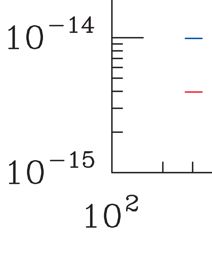
FIG. 2.: Muon neutrino plus antineutrino flux (black line), the effect of its attenuation for $\theta=0^{\circ}$ (red line) and tau neutrino plus antineutrino upward flux for the same initial flux and the same nadir angle (blue line) for a) $E^{-1}$ flux b) $E^{-2}$ flux c) AGN_SS and d) AGN_M95.

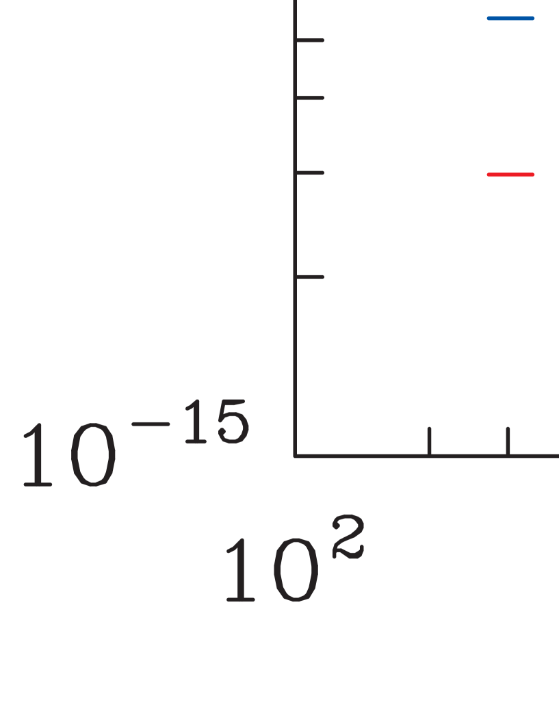
FIG. 3.: Muon neutrino plus antineutrino flux (black line), the effect of its attenuation for $\theta=0^{\circ}$ (red line) and tau neutrino plus antineutrino upward flux for the same initial flux and the same nadir angle (blue line) for a) TD_WMB, b) TD_SLSC, c) GRB_WB and d) the atmospheric flux ATMOS.

FIG. 4.: The energy dependence of the muon neutrino flux (red line) and the tau neutrino flux (blue line) for nadir angle $\theta=0^{\circ}$, $\theta=30^{\circ}$ and $\theta=60^{\circ}$ normalized to the initial flux for the AGN_M95.

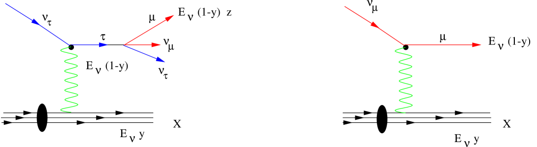
FIG. 5.: Diagrams for neutrino interactions contributing to the muon production.

FIG. 6.: Muon event rate as a function of nadir angle for energies 1 TeV, 10 TeV and 100 TeV. Muon rates including the contribution from tau decay (blue line) compared with the background from muon neutrinos (red line) for a) $E^{-1}$ flux and b) $E^{-2}$ flux.

FIG. 7.: Muon event rate as a function of nadir angle for energies 1 TeV, 10 TeV and 100 TeV. Muon rates including the contribution from tau decay (blue line) compared with the background from muon neutrinos (red line) for a) AGN_SS and b) AGN_M95.

FIG. 8.: Muon event rate as a function of nadir angle for energies 1 TeV, 10 TeV and 100 TeV. Muon rates including contribution from tau decay (blue line) compared with the background from muon neutrinos (red line) for a) TD_WMB and b) TD_SLSC.

FIG. 9.: Muon event rate as a function of nadir angle for energies 1 TeV, 10 TeV and 100 TeV. Muon rates including the contribution from tau decay (blue line) compared with the background from muon neutrinos (red line) for GRB_WB.

FIG. 10.: Muon event rate as a function of nadir angle for energies 1 TeV, 10 TeV and 100 TeV for a) Atmospheric muon neutrino and b) Atmospheric tau neutrino.

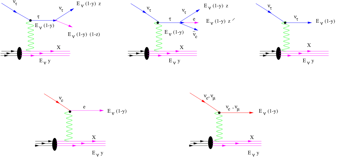
FIG. 11.: Diagrams for neutrino interactions contributing to the shower events.

FIG. 12.: Hadronic/EM event rates as a function of nadir angle for $E_{\rm shr}^{\rm min}=$1 TeV, 10 TeV and 100 TeV. Hadronic/EM event rates from $\nu_{\tau}$ (blue line) compared hadronic/EM event rates from $\nu_{\mu}$ plus $\nu_{e}$ (red line) for a) $E^{-1}$ and b) $E^{-2}$.

FIG. 13.: Hadronic/EM event rates as a function of nadir angle for $E_{\rm shr}^{\rm min}=$1 TeV, 10 TeV and 100 TeV. Hadronic/EM event rate from $\nu_{\tau}$ (blue line) compared hadronic/EM event rate from $\nu_{\mu}$ plus $\nu_{e}$ (red line) for a) AGN_SS and b) AGN_M95.

FIG. 14.: Hadronic/EM event rates as a function of nadir angle for $E_{\rm shr}^{\rm min}=$ 1 TeV, 10 TeV and 100 TeV. Hadronic/EM event rates from $\nu_{\tau}$ (blue line) compared hadronic/EM event rates from $\nu_{\mu}$ plus $\nu_{e}$ (red line) for a) TD_WMB and b) TD_SLSC.

FIG. 15.: Hadronic/EM event rates as a function of nadir angle for $E_{\rm shr}^{\rm min}=$ 1 TeV, 10 TeV and 100 TeV. Hadronic/EM event rates from $\nu_{\tau}$ (blue line) compared hadronic/EM event rates from $\nu_{\mu}$ plus $\nu_{e}$ (red line) for GRB_WB.

FIG. 16.: Hadronic/EM event rates as a function of nadir angle for $E_{\rm shr}^{\rm min}=$ 1 TeV, 10 TeV and 100 TeV. Hadronic/EM event rates from $\nu_{\tau}$ (blue line) compared hadronic/EM event rates from $\nu_{\mu}$ plus $\nu_{e}$ (red line) for a) atmospheric muon neutrino and b) atmospheric tau neutrino.

FIG. 17.: Ratio of Hadronic/EM event rate of $\nu_{\tau}$ plus $\nu_{\mu}$ plus $\nu_{e}$ assuming oscillation scenario and $\nu_{\mu}$ plus $\nu_{e}$ in the standard model as a function of nadir angle for energies 1 TeV, 10 TeV and 100 TeV for a) $E^{-1}$ and b) $E^{-2}$ flux.

FIG. 18.: Ratio of Hadronic/EM event rates of $\nu_{\tau}$ plus $\nu_{\mu}$ plus $\nu_{e}$ assuming oscillation scenario and $\nu_{\mu}$ plus $\nu_{e}$ in the standard model as a function of nadir angle for energies 1 TeV, 10 TeV and 100 TeV for a) AGN_SS and b) AGN_M95 flux.

FIG. 19.: Ratio of Hadronic/EM event rate of $\nu_{\tau}$ plus $\nu_{\mu}$ plus $\nu_{e}$ assuming oscillation scenario and $\nu_{\mu}$ plus $\nu_{e}$ in the standard model as a function of nadir angle for $E_{\rm shr}^{\rm min}=$1 TeV, 10 TeV and 100 TeV for a) TD_WMB and b) TD_SLSC flux.

FIG. 20.: Ratio of Hadronic/EM event rate of $\nu_{\tau}$ plus $\nu_{\mu}$ plus $\nu_{e}$ assuming oscillation scenario and $\nu_{\mu}$ plus $\nu_{e}$ in the standard model as a function of nadir angle for energies 1 TeV, 10 TeV and 100 TeV for GRB_WB.

FIG. 21.: Ratio of Hadronic/EM event rate of $\nu_{\tau}$ plus $\nu_{\mu}$ plus $\nu_{e}$ assuming oscillation scenario and $\nu_{\mu}$ plus $\nu_{e}$ in the standard model relative to the ratio of the muon event rate of $\nu_{\tau}$ plus $\nu_{\mu}$ assuming oscillation scenario and $\nu_{\mu}$ in the standard model (see Eq. (15)) as a function of nadir angle for threshold energies 1 TeV, 10 TeV and 100 TeV.

FIG. 22.: Ratio of Hadronic/EM event rate to muon event rate for the oscillation and no-oscillation scenarios as a function of nadir angle for threshold energies (a-b) 1 TeV, (c-d) 10 TeV and (e-f) 100 TeV for the indicated fluxes.

REFERENCES

- [1] Super-Kamiokande Collaboration (Y. Fukuda et al.) Phys. Rev. Lett. 82, 2430 (1999); ibid, hep-ex/9908049; Phys. Lett. B433, 9 (1998); Phys. Lett. B436, 33 (1998); ibid, Phys. Rev. Lett. 81, 1562 (1998).
- [2] Kamiokande Collaboration, S. Hatakeyama et al., Phys. Rev. Lett. 81, 2016 (1998).
- [3] Kamiokande Collaboration, K. S. Hirata et al., Phys. Lett.B205, 416 (1988); Phys. Lett. B280, 146 (1992); Y. Fukuda et al., Phys. Lett. B335, 237 (1994).
- [4] D. Casper et al., Phys. Rev. Lett. 66, 2561 (1991); R. Becker-Szendy et al., Phys. Rev. D46, 3720 (1992).
- [5] W. W. M. Allison et al., Phys. Lett. B391, 491 (1997).
- [6] N. Fornengo, M. C. Gonzalez-Garcia and J. W. F. Valle, hep-ph/0002147.
- [7] MINOS Collaboration, E. Ables et al., “Main Injector Neutrino Oscillation Search”, FERMILAB-PROPOSAL-P-875 (1995).
- [8] K2K Collaboration, K. Nishikawa et al. “E362 KWK-PS proposal”, March 1995; Nucl. Phys. (Proc. Supp.) B59, 289 (1997).
- [9] ICARUS Collaboration, A. Rubbia et al., CERN-SPSLC-96-58 (1996).
- [10] NOE Collaboration, M. Ambrosio et al., INFN-AE-98-09 (1998).
- [11] OPERA Collaboration, K. Kodama et al., CERN/SPSC-98-25 (1998).
- [12] S. Iyer, M. H. Reno, I. Sarcevic, Phys. Rev. D61, 053003 (2000).
- [13] For a review of neutrino oscillations see, P. Fisher, B. Kayser and K. S. McFarland, Ann. Rev. Nucl. Part. Sci. 49, 481 (1999).
- [14] F. Halzen and D. Saltzberg, Phys. Rev. Lett. 81, 4305 (1998).
- [15] T. J. Weiler, W. A. Simmons, S. Pakvasa and J. G. Learned, hep-ph/9411432.
- [16] H. Athar, M. Jezabek and O. Yasuda, TMUP-HEL-0006 (2000); O. Yasuda, TMUP-HEL-0009 (2000).
- [17] J. P. Rachen and P. Meszáros, Phys. Rev. D58, 123005 (1998).
- [18] T. Stanev et al., astro-ph/0003484.
- [19] See, for example, URL http://antares.in2p3.fr/.
- [20] See, for example, URL http://www.uao.gr/ nestor/.
- [21] See, for example, URL http://amanda.berkeley.edu/.
- [22] See, for example, URL http://amanda.berkeley.edu/km3/.
- [23] S. Bottai and F. Becattini, in Proceedings of the Cosmic Ray Conference (HE 4.2.15), Salt Lake City, Utah, August 17-23, (1999); S. Bottai and F. Becattini, astro-ph/0003179.
- [24] C. E. Fichtel, et al., Astrophys. J. Suppl. 94, 551 (1994).
- [25] M. Punch, et al. (Whipple Observatory Gamma Ray Collaboration) Nature (London) 160, 477 (1992); A.D. Kerrick et al., Astrophys. J. 438, L59 (1995); J. Quinn, et al. (Whipple Observatory Gamma Ray Collaboration) IAU Circular 6169 (June 16, 1995); J. A. Gaidos, et al, Nature (London) 383, 319 (1996); J. Quinn, et al., Ap. J. Lett. 456, L63 (1996); J. H. Buckley, et al., Ap. J. 472, L9 (1996).
- [26] M. Catanese, et al., Ap. J. 501, 616 (1998).
- [27] For a discussion of the debate over the origin of high energy photons, see, e.g., J. H. Buckley, Science 279, 676 (1998); K. Mannheim, Science 279, 684 (1998); J. Rachen, astro-ph/0003282.
- [28] F. W. Stecker and M. H. Salamon, Space Sci. Rev. 75, 341 (1995).
- [29] K. Mannheim, Astropart. Phys. 3, 295 (1995).
- [30] R. Gandhi, C. Quigg, M. H. Reno and I. Sarcevic, Astropart. Phys. 5, 81 (1996).
- [31] R. Gandhi, C. Quigg, M. H. Reno and I. Sarcevic, Phys. Rev. D58, 093009 (1998).
- [32] E. Waxman and J. N. Bahcall, hep-ph/9909286; C. D. Dermer, astro-ph/0005440.
- [33] P. Mészáros and M. J. Rees, M. N. R. A. S. 258, 41P (1992); M. J. Rees and P. Mészáros Ap. J. Lett. 430, L93 (1994). For a review, see T. Piran, Phys. Rept. 314, 575 (1999).
- [34] E. Waxman and J. N. Bahcall, Phys. Rev. Lett. 78, 2292 (1997).
- [35] E. Waxman and J. N. Bahcall, Phys. Rev. D59, 023002 (1999); J. N. Bahcall and E. Waxman, hep-ph/9902383; K. Mannheim, R. J. Protheroe and J. P. Rachen, astro-ph/9812398.
- [36] G. Sigl, S. Lee, D. N. Schramm, and P. Coppi, Phys. Lett. B392, 129 (1997).
- [37] U. F. Wichoski, J. H. Macgibbon, and R. H. Brandenberger, ‘High Energy Neutrinos, Photons and Cosmic Rays from Non-Scaling Cosmic Strings,’ BROWN-HET-1115, hep-ph/9805419.
- [38] R. J. Protheroe and T. Stanev, Phys. Rev. Lett. 77, 3708 (1996).
- [39] W. Rhode et al., Astropart. Phys. 4, 217 (1996).
- [40] R. Baltrusaitis et al., Astrophys. J. Lett. 281, L9 (1984); R. Baltrusaitis Phys. Rev. D31, 2192 (1985).
- [41] V. Agrawal, T. K. Gaisser, P. Lipari and T. Stanev, Phys. Rev. D53, 1314 (1996).
- [42] C. T. Hill and D. N. Schramm, Phys. Rev. D31, 564 (1985); S. Yoshida and M. Teshima, Prog. Theor. Phys. 89, 833 (1993); R. J. Protheroe and P. A. Johnson, Astropart. Phys. 4, 253 (1996), Errat. ibid 5, 215 (1996). For a recent calculation of ultrahigh energy cosmic ray propagation, see, e.g., T. Stanev et al., Ref. [18].
- [43] D. Seckel, T. Stanev and T. Gaisser, Astrophys. J 383, 652 (1991); G. Ingelman and M. Thunman, Phys. Rev. D54, 4385 (1996); C. Hettlage, K. Mannheim and J. G. Learned, Astropart. Phys. 13, 45 (2000).
- [44] V. A. Naumov and L. Perrone, Astropart. Phys. 10, 239 (1999).
- [45] J. G. Learned and S. Pakvasa, Astropart. Phys. 3, 267 (1995); H. Athar, G. Parente and E. Zas, hep-ph/0006123; J. Alvarez-Muniz and F. Halzen, “Detection of Tau Neutrinos in IceCube,” unpublished. See also A. Husain, Nucl. Phys. Proc. Suppl. 87, 442 (2000) and hep-ph/0004083.
- [46] See, e.g., A. Breakstone et al., ISR collaboration, Phys. Rev. D30, 508 (1984).
- [47] The IceCube proposal can be found at http://pheno.physics.wisc.edu/icecube.
- [48] A. Dziewonski, Earth Structure, Global, in Encyclopedia of Solid Earth Geophysics, ed. David E. James (Van Nostrand Reinhold, New York, 1989) pg. 331.
- [49] P. Lipari and T. Stanev, Phys. Rev. D44, 3543 (1991).
- [50] H. L. Lai et al. (CTEQ Collaboration), Eur. Phys. J. C12, 375 (2000).
- [51] L. Pasquali and M. H. Reno, Phys. Rev. D59, 093003 (1998).
- [52] The energy spectra of neutrino induced showers for TeV, in the context of neutrino oscillations of atmospheric neutrinos, appears in T. Stanev, Phys. Rev. Lett. 83, 5427 (1999).
- [53] J. G. Learned, private communications.
- [54] S. Markoff, F. Melia and I. Sarcevic, Astrophys. J. 522, 870 (1999).
- [55] T. K. Gaisser, Cosmic Rays and Particle Physics, (Cambridge University Press, Cambridge, 1990).
- [56] P. Lipari, Astropart. Phys. 1, 195 (1993).