Four-Fermion Production in Electron-Positron Collisions

• Institut für Physik, Humboldt-Universität zu Berlin, Germany

• Dipartimento di Fisica Teorica, Università di Torino, Torino, Italy

• INFN, Sezione di Torino, Torino, Italy

• Paul Scherrer Institut, Villigen, Switzerland

• LAL, B.P. 34, F-91898 Orsay Cedex

• CERN, EP Division, CH-1211 Geneva 23, Switzerland

• LNP, JINR, RU-141980 Dubna, Russia

• Physics Department, University of Durham, Durham, England

• Instituut-Lorentz, University of Leiden, The Netherlands

• Institute of Nuclear Physics, Moscow State University, Moscow, Russia

• Theoretische Physik, Universität Bielefeld, Bielefeld, Germany

• DESY, Theory Division, D-22603 Hamburg, Germany

• High Energy Accelerator Research Organization, Tsukuba, Japan

• Institute of Physics, Meiji-Gakuin University, Yokomama, Japan

• Dipartimento di Fisica Teorica e Nucleare, Università di Pavia, Italy

• INFN, Sezione di Pavia, Pavia, Italy

• Dipartimento di Fisica, Università di Ferrara, INFN, sezione di Ferrara

• Insitute of Nuclear Physics, NCSR ‘Democritos’, 15310 Athens, Greece

• University College, London, England

• Theory Group, DESY, D-15738 Zeuthen, Germany

• Institut für Theoretische Physik, Universität Leipzig, Leipzig, Germany

• RWTH Aachen, Germany

• LPNHE, Ecole Polytechnique, F-91128 Palaiseau CEDEX, FRANCE

• Department of Physics and Astronomy, University of Rochester, Rochester NY, USA

• Institute of Nuclear Physics, ul. Kawiory 26a, 30-055 Cracow, Poland

• CERN, Theory Division, CH-1211 Geneva 23, Switzerland

• Institute of Computer Science, Jagellonian University,
  ul. Nawojki 11, 30-072 Cracow, Poland

• Department of Physics and Astronomy,
  The University of Tennessee, Knoxville, Tennessee 37996-1200, USA

• SLAC, Stanford University, Stanford, California 94309, USA

• previously at Rutherford Appleton Lab, United Kingdom

The LEP-2 Monte Carlo Workshop 1999/2000

Four-Fermion Production in Electron-Positron Collisions

Four-Fermion Working Group Report

Abstract

This report summarises the results of the four-fermion working group of the LEP2-MC workshop, held at CERN from 1999 to 2000. Recent developments in the calculation of four-fermion processes in electron-positron collisions at LEP-2 centre-of-mass energies are presented, concentrating on predictions for four main reactions: W-pair production, visible photons in four-fermion events, single-W production and Z-pair production. Based on a comparison of results derived within different approaches, theoretical uncertainties on these predictions are established.

1 Introduction

During the year 1999 an informal workshop on Monte Carlo (MC) generators and programs took place at CERN, concentrating on processes in $e^{+}e^{-}$ interactions at LEP 2 centre-of-mass energies (161 GeV to 210 GeV). One of the goals was to summarize and review critically the progress made in theoretical calculations and their implementation in computer programs since the 1995 workshop on Physics at LEP2. One of the reasons for this report was the need of having an official statement on various physics processes and the accuracy of their predictions, before deciding on LEP 2 activities in the year 2000.

This part of the workshop report summarizes the findings in the area of Four-Fermion final states. At the beginning of the workshop the following goals were identified for the Four-Fermion sub-group:

• Describe the new calculations and improvements in the theoretical understanding and in the upgraded MC implementations.

• Indicate where new contributions have changed previous predictions in the MC adopted by the collaborations, and specify why, how and by how much.

• In those cases where a substantial discrepancy has been registered and the physical origin has been understood, recommendations should be made on what to use.

• In those cases where we have found incompleteness of the existing MC, but no complete improvement is available, we should be able to indicate a sound estimate of the theoretical uncertainty, and possibly way and time scale for the solution.

Our strategy is determined by the physics issues arising in the experimental analyses performed at LEP 2. Therefore, the four LEP Collaborations have been asked to provide a list of relevant processes together with the level of theoretical accuracy needed.

Clearly, the LEP experiments investigate many different processes. For theoretical predictions we thus have to manage with lots of different sets of cuts. At the beginning of our activities the four experiments have presented us with lists that reflect rather diverse styles and different approaches: The complexity of the observables varied greatly, ranging from those defined by simple phase-space cuts on four-fermion (+ photon) level to complete event-selection procedures requiring parton shower and hadronization of quark systems.

An effort was made to settle as much as possible on a set of quasi-realistic but simple cuts for each process. We have collected processes and/or phase space regions where improved theoretical predictions are desirable. A weight has been assigned to each process according to its relevance and urgency.

The focus of activity has been on improving the theoretical predictions for the relevant processes and/or phase space regions. Also, all contributors have been asked to give an estimate for the remaining theoretical uncertainty. As a consequence, the output of the whole operation should not be a mere collection of comparison tables but a coherent attempt in assessing the theoretical uncertainty to be associated to any specific process.

The realm of theoretical uncertainty is ill defined and in order to reach a general consensus one cannot be satisfied with just some statement on the overall agreement among different programs. Whenever differences are found, one has to make sure that they are due to physics, and not to some different input. So our project had to foresee a preliminary phase with more of a technical benchmark. Once trivial discrepancies are understood and sorted out, one can start digging into inevitable differences arising from different implementations of common theoretical wisdom.

In a vast majority of cases the main theoretical problem is represented by the inclusion of QED radiation. Therefore, one of the main questions was: can we improve upon our treatment of QED radiation and/or give some safe estimate of the theoretical uncertainty associated with it?

Below we will present our reference table of four-fermion processes. It is an idealised common ground where, in principle, all theoretical predictions should be compared. More advanced setups would be accessible only to a more limited number of generators, built for that specific purpose.

It is useful to recall that the ultimate, perfect program does not exist and, most likely, will never exist. Roughly speaking, programs belong to two quite distinct classes. On one side there are event generators, usually interfaced with parton shower and hadronization packages. They may miss some fine points of the theoretical knowledge but represent an essential ingredient in the experimental analyses concerning the evaluation of signal efficiencies and backgrounds. Thus they create the necessary bridge between the raw data recorded by the detectors and the background-subtracted efficiency-corrected results published. At the other end of this cosmos we have semi-analytical programs that are not meant to generate events. Rather, they show their power in dealing with the signal, furnishing the implementation of (almost) everything available in the literature concerning the calculation of specific processes. In either case, we want to know about the theoretical uncertainty, process by process, to make clear which program is able to achieve that level of accuracy under which configuration. For $W$-pair production, however, the scenario is slightly changed: We have now MC event generators that, at the same time, represent a state-of-the-art calculation. Nevertheless, we do not have yet the ultimate MC: the one with radiative corrections, virtual/soft/hard photons, DPA, complete phase-space including single-$W$, single-$Z$, $Z\gamma^{*}$ and able to produce weight-1 events in finite time.

The results presented in this report are based on several different approaches and on comparisons of their numerical predictions. They are calculated with the following computer codes: BBC, CompHEP, GENTLE, grc4f, KORALW/YFSWW/YFSZZ, NEXTCALIBUR, PHEGAS/HELAC, RacoonWW, SWAP/WRAP, WPHACT and WTO/ZZTO.

This article is organised as follows. In Sect. 2 we present the four-fermion processes looked at in detail. Then we review the most recent theoretical developments in four-fermion physics in $e^{+}e^{-}$ interactions. In Sect. 4 we discuss the CC03 $\sigma_{{\scriptscriptstyle{W}}{\scriptscriptstyle{W}}}$ cross-section and predictions based on the DPA. Here different approaches are compared. In Sect. 5 we discuss the radiative process with $4{\rm f}+\gamma$ final states. In Sect. 6 the single-$W$ production is critically discussed. Finally the NC02 cross-section, $\sigma_{{\scriptscriptstyle{Z}}{\scriptscriptstyle{Z}}}$ is analysed in Sect. 7 Conclusions and outlook are presented in Sect. 8

2 Four-fermion processes

Here we present our basic reference table and specify the calculational setup. One should read it as summarizing our original manifest. After reading the following sections, it will be instructive to come back here with a critical eye: not all the items and questions listed below have found a satisfactory answer. This was, somehow, foreseeable. If one thinks carefully one will easily discover some important message also for those issues that remain unsolved: they cannot be solved in any reasonable time scale and the associated effect is a real source of uncertainty.

2.1 List of processes

The following list provides the observables together with precision tags in $\%$, as requested by the experimental Collaborations. The accuracy of MC simulations should be better than the requested precision tag, i.e. the physics uncertainty should be smaller and at worst the one indicated. How much better is left to the contributors. For benchmarking it is certainly advisable to use the maximum available precision.

In general, radiative corrections and radiative photons in the final state should be considered for all processes, including the discussion of photon energy and polar-angle spectra. Typical minimal requirements on real photons are: energy $E_{\gamma}>1\,$GeV; polar angle $|\cos\theta_{\gamma}|<0.985,0.997,0.9995$ depending on channel; and minimal angle between photon and any charged final-state fermion $\xi>5^{\circ}$.

• $WW$ and $ZZ$ type signal:

1. $e^{+}e^{-}\rightarrow WW\rightarrow\,$ all (CC03). The full phase space is needed and the inclusive cross-section accuracy is $0.2\%$, which is $1/3$ of experimental accuracy combining all LEP 2 energies,

   The spectrum for the photon energy and the polar angle is needed ($|\cos\theta_{\gamma}|<0.985~{}(0.997)$).

2. $e^{+}e^{-}\rightarrow ZZ\rightarrow\,$ all (NC02). The full phase space is needed and the inclusive cross-section accuracy is $1\%$. The spectrum for the photon energy and the polar angle is needed ($|\cos\theta_{\gamma}|<0.985~{}(0.997)$).

3. $e^{+}e^{-}\rightarrow l\nu l\nu(\gamma)$ where all $\{e/\mu/\tau\}\,\otimes\{e/\mu/\tau\}$ combinations are requested with the following conditions: ($|\cos\theta_{l_{1}/l_{2}}|<0.985$, $E_{l_{1}/l_{2}}>5\,$GeV, $M(l^{+}l^{-})>10~{}(45)\,$GeV (full and high-mass region). The inclusive cross-section accuracy is $4\%$ for individual combination; the inclusive cross-section accuracy is $1\%$ for the summed one; photon energy and polar angle spectrum ($|\cos\theta_{\gamma}|<0.985~{}(0.997)$).

4. $e^{+}e^{-}\rightarrow\overline{q}qe\nu(\gamma)$ (CC20), $q$-flavour blind, $|\cos\theta_{e}|<0.985$, $E_{e}>5\,$GeV, $M(q\overline{q})>10~{}(45)\,$GeV (full and high-mass region); inclusive cross-section accuracy is $1\%$ (5% for low-mass region); photon energy and polar angle spectrum ($|\cos\theta_{\gamma}|<0.985~{}(0.997)$).

5. $e^{+}e^{-}\rightarrow\overline{q}q\mu\nu(\gamma)$ and $e^{+}e^{-}\rightarrow\overline{q}q\tau\nu(\gamma)$ (incl. tau polarization in tau decay) (CC10), $|\cos\theta_{\mu/\tau}|<0.985,E_{\mu/\tau}>5\,$GeV, $M(q\overline{q})>10~{}(45)\,$GeV (full and high-mass region), inclusive cross-section accuracy $1\%$. Photon energy and polar angle ($|\cos\theta_{\gamma}|<0.985~{}(0.997)$) spectrum.

6. $e^{+}e^{-}\rightarrow q\overline{q}q\overline{q}(\gamma)$, flavour blind, $bbq\overline{q}$, $bbbb$. At least two pairs with $M(q_{i},q_{j})>10~{}(45)\,$GeV (full and high-mass region), inclusive cross-section accuracy $1\%$. photon energy and polar angle ($|\cos\theta_{\gamma}|<0.985~{}(0.997)$) spectrum.

7. $e^{+}e^{-}\rightarrow q\overline{q}l^{+}l^{-}(\gamma)$, $q$-flavour blind, heavy $q$-flavors, $l=e/\mu/\tau$, $|\cos\theta_{l_{1}}|<0.985$, no cut on 2nd lepton (only one lepton tagged), $M(q\overline{q})>10~{}(45)\,$GeV (full and high-mass region), inclusive cross-section accuracy $2\%$. Photon energy and polar angle ($|\cos\theta_{\gamma}|<0.985~{}(0.997)$) spectrum.

8. $e^{+}e^{-}\rightarrow q\overline{q}l^{+}l^{-}(\gamma)$, $q$-flavour blind, heavy $q$-flavors, $|\cos\theta_{l_{1}}|,|\cos\theta_{l_{2}}|<0.985$ (both leptons tagged), full and high-mass regions: $M(l^{+}l^{-})>10~{}(45)\,$GeV, $M(q\overline{q})>10~{}(45)\,$GeV, inclusive cross-section accuracy $2\%$. Photon energy and polar angle ($|\cos\theta_{\gamma}|<0.985~{}(0.997)$) spectrum.

9. $e^{+}e^{-}\rightarrow q\overline{q}e^{+}e^{-}(\gamma)$, $q$-flavour blind, heavy $q$-flavors, with one electron in the beam pipe, $|\cos\theta_{e}|>0.997$, and one electron tagged, $|\cos\theta_{e}|<0.985$, $M(q\overline{q})>10~{}(45)\,$GeV (full and high-mass region) . Photon energy and polar angle ($|\cos\theta_{\gamma}|<0.985~{}(0.997)$) spectrum.

10. $e^{+}e^{-}\rightarrow q\overline{q}\nu\overline{\nu}(\gamma)$, $q$-flavour blind, heavy $q$-flavors, $M(q\overline{q})>10~{}(45)\,$GeV, inclusive cross-section accuracy $4\%$ (10% for low-mass region). Photon energy and polar angle ($|\cos\theta_{\gamma}|<0.985~{}(0.997)$) spectrum.

11. $e^{+}e^{-}\rightarrow l^{+}l^{-}L^{+}L^{-}(\gamma)$ and $e^{+}e^{-}\rightarrow l^{+}l^{-}l^{+}l^{-}(\gamma)$ (all possible charged lepton flavour combinations): 3 or 4 leptons within acceptance $|\cos\theta|<0.985$, $M(l^{+}l^{-})$ and $M(L^{+}L^{-})>10~{}(45)\,$GeV (full and high-mass region). Photon energy and polar angle ($|\cos\theta_{\gamma}|<0.985~{}(0.997)$) spectrum.

• Single-$W$ type signal:

1. $e^{+}e^{-}\rightarrow q\overline{q}e\nu(\gamma)$, $|\cos\theta_{e}|>0.997$, either $M(q\overline{q})>45\,$GeV or $E_{q_{1}},E_{q_{2}}>15\,$GeV, inclusive cross-section accuracy $3\%$, photon energy and polar angle ($|\cos\theta_{\gamma}|<0.997~{}(0.9995)$) spectrum.

2. $e^{+}e^{-}\rightarrow e\nu e\nu(\gamma)$, $|\cos\theta_{e}|>0.997$, $E_{e}>15\,$GeV, $|\cos\theta_{e}|<0.7~{}(0.95)$, inclusive cross-section accuracy $5\%$, photon energy and polar angle ($|\cos\theta_{\gamma}|<0.997~{}(0.9995)$) spectrum.

3. $e^{+}e^{-}\rightarrow e\nu\mu\nu(\gamma)$ and $e^{+}e^{-}\rightarrow e\nu\tau\nu(\gamma)$, $|\cos\theta_{e}|>0.997$, $E_{\mu/\tau}>15\,$GeV, $|\cos\theta_{\mu/\tau}|<0.95$, inclusive cross-section accuracy $5\%$, photon energy and polar angle ($|\cos\theta_{\gamma}|<0.997~{}(0.9995)$) spectrum.

This list deserves already few words of comment.

For hadronic systems (CC or NC), there is usually a requirement of at least $45$ GeV invariant mass ($W$ and $Z$ signal) or at least $10$ GeV (background for other processes). Even lower invariant masses, say down to $1\,$GeV, should be handled by the dedicated $\gamma\gamma$ subgroup. For leptons, there should be no problem to go down to lower invariant masses or energies than listed above.

We consider as radiative events those events with real photons where at least one photon passes the photon requirements listed above, and as non-radiative events those with no photon or only photons below the minimal photon requirements. In case of non-radiative and radiative events, the cross section and its accuracy is needed. In case of non-radiative events, this amounts to adding up virtual and soft radiative corrections. In case of radiative events, some distributions are needed in addition, in particular photon energy and polar angle, and photon angle with respect to the nearest charged final-state fermion.

2.2 Questions to theory

We now elaborate in more detail on specific questions associated to specific processes.

• ${\mathcal{O}}(\alpha)$ electroweak corrections to $e^{+}e^{-}\rightarrow WW\rightarrow 4\,{\rm f}$.

Until 1999, the LEP experiments were using a $2\%$ theoretical uncertainty on the calculation of the CC03 $W$-pair cross section, not changed since the 1995 LEP 2 workshop. Although no complete one-loop ${\mathcal{O}}\left(\alpha\right)$ EW calculation exist yet for off-shell $e^{+}e^{-}\rightarrow WW\rightarrow 4\,$f production, we wish the theoretical uncertainty to be below $1\%$ ($0.5\%$ if possible) with justification. Also the uncertainties in CC03 vs. $4{\rm f}$ corrections when measuring the $WW$ cross section should be understood.

• Photon radiation (ISR) with $p_{t}$ in $WW$ and $ZZ$-dominated channels.

The principle effects will be on the selection efficiency and on the differential distributions used for W mass and triple gauge boson coupling (TGC) studies. The interest in photons is twofold: photons explicitly identified as such - usually at larger polar angles - and photons which simply create noticeable activity in the detector. The latter is, for example, also important in single-$W$ type analysis, therefore the photon angular range is extended to very low polar angles.

• Single $W$ channels.

For the single-$W$ process there are several issues to be addressed. In the region of high invariant masses of the $W$ boson (above $45\,$GeV) this process is important for both searches and TGC measurements. One topic of investigation should be ISR: this process is dominated by $t$-channel diagrams, whereas the current MC program implement ISR assuming s-channel reactions. A second issue is the treatment of the $\alpha_{\rm QED}$ scale, not only for single-$W$ but also for single-$Z$ and for $Z\gamma^{*}$. Is it better to re-weight on a event by event basis or on a diagram basis?

One of the outcomes of the workshop should be a recommendation on the mass cut which distinguishes the high mass region (more reliable) from the low mass region, i.e. the lower value to which the $5\%$ (or better) precision tag applies.

The importance of ISR in this channel is threefold: (a) change in total cross-section due to normal radiative corrections, (b) change in event distributions used to make cuts which changes the fraction of the total that fall inside our cuts, (c) fraction of events with identified photons - this forms a background to some of the chargino searches where a detected gamma is required.

Since the single-$W$ topology is defined as the one where a high mass object is found in the detector and the electron is not observed, we would like to know how the presence of $p_{t}$ ISR changes the fraction of events where the electron gets kicked out of the beam-pipe, how the differential distributions are distorted for TGC studies and what the explicit hard photon rate is.

The low mass region (below $45$ GeV) is mostly important for searches and studied within the $\gamma\gamma$ sub-group. One would like to trust the MC predictions down to $5-10\,$GeV invariant mass for the hadronic system. The required precision should also be around $5$ to $10\%$.

2.3 Input parameter set

A set of parameters must be specified for the calculation of ${\mathcal{O}}\left(\alpha\right)$ predictions (CC03 and to some extent also NC02). Once radiative corrections are included, the question of Renormalization Scheme (RS) and of Input Parameter Set (IPS) becomes relevant. For calculation, the following input parameters are used:

$$M_{{}_{Z}} = 91.1867\,\,\mathrm{GeV},\quad 1/\alpha(0)=137.0359895,$$

$$G_{{\scriptscriptstyle{F}}} = 1.16637\times 10^{-5}\,\,\mathrm{GeV}^{-2}.$$ (1)

As far as masses are concerned one should use:

Leptons:

PDG values, i.e.

$$m_{e} = 0.51099907\,\,\mathrm{MeV},\quad m_{\mu}=105.658389\,\,\mathrm{MeV},$$

$$m_{\tau} = 1.77705\,\,\mathrm{GeV}.$$ (2)

Quarks:

for light quarks one should make a distinction; for phase space:

$$m_{u}=5\,\,\mathrm{MeV},\qquad m_{d}=10\,\,\mathrm{MeV},\qquad\mbox{only relevant for single-}W,$$ (3)

while, in principle, these masses should not be used in deriving $\alpha_{\rm QED}(s)$ from $\alpha_{\rm QED}(0)$.

Here the recommendation follows the agreement in our community on using the following strategy for the evaluation of $\alpha_{\rm QED}$ at the mass of the $Z$. Define:

$$\alpha(M_{{}_{Z}})=\frac{\alpha(0)}{1-\Delta\alpha^{(5)}(M_{{}_{Z}})-\Delta_{\rm{top}}(M_{{}_{Z}})-\Delta^{\alpha\alpha_{{}_{S}}}_{\rm{top}}(M_{{}_{Z}})}\;,$$ (4)

where one has $\Delta\alpha^{(5)}(M_{{}_{Z}})=\Delta\alpha_{\rm{lept}}+\Delta\alpha^{(5)}_{\rm{had}}$.

The input parameter should be $\Delta\alpha^{(5)}_{\rm{had}}$, as it is the contribution with the largest uncertainty, while the calculation of the top contributions to $\Delta\alpha$ is left for the code. This should become common to all codes. Codes should include, for $\Delta\alpha_{\rm{lept}}$, the recently computed ${\mathcal{O}}\left(\alpha^{3}\right)$ terms of [1] and use as default $\Delta\alpha^{(5)}_{\rm{had}}=0.0280398$, taken from [2]. Using the default one obtains $1/\alpha^{(5)}(M_{{}_{Z}})=128.877$, to which one must add the $t\overline{t}$ contribution and the ${\mathcal{O}}\left(\alpha\alpha_{{}_{S}}\right)$ correction induced by the $t\overline{t}$ loop with gluon exchange, [3]. Therefore, light quark masses should not appear in the evaluation of $\alpha_{\rm QED}(M_{{}_{Z}})$ and one should end up with:

$$1/\alpha(M_{{}_{Z}}) = 128.887,$$

for $$M_{{}_{Z}}=91.1867\,GeV,\quad m_{t}=175\,\,\mathrm{GeV},$$ (5)

$$M_{{}_{H}}=150\,\,\mathrm{GeV},\quad\alpha_{{}_{S}}(M_{{}_{Z}})=0.119.$$

Furthermore, one should use:

$$\alpha_{{}_{S}}(M_{{}_{Z}})=0.119,\quad M_{{}_{H}}=150\,\,\mathrm{GeV},\quad M_{{}_{W}}=80.350\,\,\mathrm{GeV}.$$ (6)

The quantities $\Gamma_{{}_{Z}},\Gamma_{{}_{W}}$ should be understood as computed in the minimal standard model, e.g. $\Gamma_{{}_{Z}}=2.49471\,\,\mathrm{GeV}$ and $\Gamma_{{}_{W}}=2.08699\,\mathrm{GeV}$ for our IPS.

Now we come to the most important point, what to do with IPS in the presence of radiative corrections. In principle, all RS and all IPS are equally good and accepted, and differences are true estimates of some component of the theoretical uncertainty. However, we want to make sure that differences are not due to technical precision. The IPS that we want to specify is over-complete, let us repeat,

$$G_{{\scriptscriptstyle{F}}} = 1.16637\times 10^{-5}\,\,\mathrm{GeV}^{-2},\qquad 1/\alpha(M_{{}_{Z}})=128.887,$$

$$M_{{}_{Z}} = 91.1867\,\,\mathrm{GeV},\qquad M_{{}_{W}}=80.350\,\,\mathrm{GeV},$$

$$\alpha_{{}_{S}}(M_{{}_{Z}}) = 0.119,\qquad M_{{}_{H}}=150\,\,\mathrm{GeV}.$$ (7)

Clearly, once radiative correction are on, $s_{\theta}=s_{\theta}^{\rm xxx-scheme}$ and we don’t care anymore since enough radiative corrections should be included to make all schemes equivalent to ${\mathcal{O}}\left(\alpha\right)$. Thus, for ${\mathcal{O}}\left(\alpha\right)$ numbers $s_{\theta}$ drops out. Perhaps we should give the highest marks to schemes where $M_{{}_{W}}$ is in the IPS; after all, experiments measure $M_{{}_{W}}$ at LEP 2 and any scheme where $M_{{}_{W}}$ is not a primary quantity in the IPS is as bad as a scheme for LEP 1 where $M_{{}_{Z}}$ is a derived quantity.

Nevertheless, we can use the over-completeness of the present IPS to set some internal consistency: it is a good idea to have an over-complete set of IPS, nevertheless consistent, so that everybody can make his favourite choice of the RS. Since we include values for $\alpha(M_{{}_{Z}})$ and for $G_{{\scriptscriptstyle{F}}}$ we can, as well, fine-tune the numbers so that the internal relations hold, to the best of our knowledge. The recommendation, in this case, is as follows:

• write down your favorite equation

  $$f\left(M_{{}_{Z}},M_{{}_{W}},m_{t},M_{{}_{H}},\alpha_{{}_{S}}(M_{{}_{Z}}),\alpha(0),G_{{\scriptscriptstyle{F}}}\right)=0,$$ (8)

• keep everything fixed but $m_{t}$ which, in turn, is derived as a solution of the consistency equation (for OMS this involves typically $\Delta r$).

Even this solution is RS-dependent but variation should be minimal, sort of irrelevant. For instance, one could use the following result (derived from TOPAZ0 [4]):

$$m_{t}=174.17\,\,\mathrm{GeV}\quad\mbox{Default for CC03}\,\,\,{\mathcal{O}}\left(\alpha\right).$$ (9)

With $M_{{}_{W}}=80.350\,GeV$ and $M_{{}_{H}}=150\,$GeV we are in a lucky situation, $m_{t}$ doesn’t change too much. For more solutions, we refer to Tab.(1).

$M_{{}_{H}}\,[\,\mathrm{GeV}]$	$m_{t}\,[\,\mathrm{GeV}]$
100	170.03
150	174.17
180	176.14
250	179.90

Table 1: $m_{t}$ as a function of $M_{{}_{H}}$.

2.4 Comparisons for $4\,{\rm f}$ results

There is an old tradition in LEP physics, new theoretical ideas and improvements should always be cross-checked before being adopted in the analysis of the experimental data. In this Report we present accurate and detailed comparisons between different generators. In most cases the authors have agreed to coordinate their action in understanding the features of the generators, their intrinsic differences and the goodness of their agreement or disagreement for the predictions. In so doing, and for the attuned comparisons, they can exclude that eventual disagreement may originate from trivial sources, like different input parameters.

Before entering into a detailed study of the numerical results it is important to underline how an estimate of the theoretical uncertainty emerges from the many sets of numbers obtained with the available generators. First of all one may distinguish between intrinsic and parametric uncertainties. The latter are normally associated with a variation of the input parameters according to the precision with which they are known. These uncertainties will eventually shrink when more accurate measurements will become available.

In this Report we are mainly devoted to a discussion of the intrinsic uncertainties associated with the choice of one scheme versus another. With one generator alone one cannot simulate the shift of a given quantity due to a change in the renormalization scheme. Thus the corresponding theoretical band in that quantity should be obtained from the differences in the prediction of the generators. On top of that we should also take into account the possibility of having different implementations of radiative corrections within one code. Many implementations of radiative corrections and of DPA are equally plausible and differ by non-leading higher order contributions, which however may become relevant in view of the achieved or projected experimental precision. This sort of intrinsic theoretical uncertainty can very well be estimated by staying within each single generator. However, since there are no reasons to expect that these will be the same in different generators, only the full collection of different sources will, in the end, give a reliable information on how accurate an observable may be considered from a theoretical point of view.

3 Phenomenology of unstable particles

In order to extract the $WW$ signal from the full set of ${\mathrm{e^{+}}}{\mathrm{e^{-}}}\rightarrow 4f$ processes, the CC03 cross-section was introduced and discussed in [5]. In lowest order, this cross-section is simply based on the three $WW$ signal diagrams with the full four-particle kinematics with off-shell $W$ bosons. Compared to the full set of diagrams, the CC03 subset depends only trivially on the final state and allows to combine all channels easily. However, since the CC03 cross-section is based on a subset of diagrams, it is gauge-dependent and usually defined in the ’t Hooft–Feynman gauge. While the CC03 cross-section is not an observable, it is nevertheless a useful quantity at LEP 2 energies where it can be classified as a pseudo-observable. It contains the interesting physics, such as the non-abelian couplings and the sensitivity of the total cross section to $M_{{}_{W}}$ near the $W$-pair threshold. The goal of this common definition is to be able to combine the different final state measurements from different experiments so that the new theoretical calculations can be checked with data at a level better than $1\%$. Note, however, that the CC03 cross-section will become very problematic at linear-collider energies, where the background diagrams and the gauge dependences are much larger.

It is worth summarizing the status of the $WW$ cross-section prior to the 2000 Winter Conferences. Nominally, any calculation for ${\mathrm{e^{+}}}{\mathrm{e^{-}}}\rightarrow{\mathrm{W}}{\mathrm{W}}\rightarrow 4f$ was a tree level calculation and one could try the standard procedure of including, in a reasonable way, as much as possible of the universal corrections by constructing an improved Born approximation (hereafter IBA). This is the way the data have been analyzed so far, mostly with the help of GENTLE. Different programs have been compared for CC03, see Ref. [5]: when one puts the same input parameters, renormalization scheme, etc, a technical agreement at the $0.1\%$ level is found. The universal corrections are not enough, since we wish the theoretical uncertainty to be below $1\%$ ($0.5\%$ seems possible) with justification.

Indeed, we have clear indications that non-universal electroweak corrections for $WW$(CC03) cross-section are not small and even larger than the experimental LEP accuracy. GENTLE will produce a CC03 cross-section, typically in the $G_{{\scriptscriptstyle{F}}}$-scheme, with universal ISR QED and non-universal ISR/FSR QED corrections, implemented with the so-called current-splitting technique. The corresponding curve has been used for the definition of the Standard Model prediction with a $\pm 2\%$ systematic error assigned to it. This error estimate [42, 133] is based on the knowledge of both leading and full ${\mathcal{O}}\left(\alpha\right)$ corrections to on-shell $W$-pair production. Note that, in GENTLE, the non-universal ISR correction with current-splitting technique reads as $+0.4\%$ effect at LEP 2 energies.

Recently, a new electroweak ${\mathcal{O}}\left(\alpha\right)$ CC03 cross-section has become available, in the framework of DPA, showing a result that is $2.5\div 3\%$ smaller than the CC03 cross-section from GENTLE. This is a big effect since the combined experimental accuracy of LEP experiments is even smaller. It is, therefore, of the upmost importance to understand the structure of a DPA-corrected CC03 cross-section.

The double-pole approximation (DPA) of the lowest-order cross-section emerges from the CC03 diagrams upon projecting the $W$-boson momenta in the matrix element to their on-shell values. This means that the DPA is based on the residue of the double resonance, which is a gauge-invariant quantity, because it is directly related to the sub-processes of on-shell $W$-pair production and on-shell $W$ decay. In contrast to the CC03 cross-section, the DPA is theoretically well-defined. The price to be paid for this is the exclusion of the threshold region, where the DPA is not valid. On the other hand, the DPA provides a convenient framework for the inclusion of radiative corrections.

3.1 Dealing with unstable particles

Most of our technical problems originate from the complications naturally pertaining to the gauge structure of the theory and to the presence of unstable particles. As an interlude, we would like to summarize the nominal essence of the theoretical basis of all generators. In this respect one should remember that several, new, theoretical ideas were fully developed also as a consequence of the previous workshop on $WW$-physics (Physics at LEP2, Yellow report CERN/96-01, February 1996) and, in turn, many generators have profited from the most recent theoretical development. Furthermore, this Section will be a natural place where to add some consideration about the fine points in the DPA-procedure.

Four-fermion production processes, with or without radiative corrections, all involve fermions in the initial and final state and unstable gauge bosons as intermediate particles. Sometimes a photon is also present in the final state. If complete sets of graphs contributing to a given process are taken into account, the associated matrix elements are in principle gauge-invariant, i.e. they are independent of gauge fixing and respect Ward identities. This is, however, not guaranteed for incomplete sets of graphs like the ones corresponding to the off-shell $W$-pair production process (CC03). Indeed this process has been found to violate the $SU(2)$ Ward identities [6].

In addition, the unstable gauge bosons that appear as intermediate particles can give rise to poles $1/(p^{2}-M^{2})$ in physical observables if they are treated as stable particles. In view of the high precision of the LEP 2 experiments, the proper treatment of these unstable particles has become a demanding exercise, since on-shell approximations are simply not good enough anymore. A proper treatment of unstable particles requires the re-summation of the corresponding self-energies to all orders. In this way the singularities originating from the poles in the on-shell propagators are regularized by the imaginary parts contained in the self-energies, which are closely related to the decay widths ($\Gamma$) of the unstable particles. The perturbative re-summation itself involves a simple geometric series and is therefore easy to perform. However, this simple procedure harbours the serious risk of breaking gauge invariance. Gauge invariance is guaranteed order by order in perturbation theory. Unfortunately one takes into account only part of the higher-order terms by re-summing the self-energies. This results in a mixing of different orders of perturbation theory and thereby jeopardizes gauge invariance, even if the self-energies themselves are extracted in a gauge-invariant way. Apart from being theoretically unacceptable, gauge-breaking effects can also lead to large errors in the MC predictions. At LEP 2 energies this problem occurs for instance in the reactions $\,e^{+}e^{-}\rightarrow e^{-}\overline{\nu}_{e}u\overline{d},\,e^{+}\nu_{e}\overline{u}d\,$ for forward-scattered beam particles [7].

Based on this observation, it is clear that a gauge-invariant scheme is required for the treatment of unstable particles. It should be stressed, however, that any such scheme is arbitrary to a greater or lesser extent: since the Dyson summation must necessarily be taken to all orders of perturbation theory, and we are not able to compute the complete set of all Feynman diagrams to all orders, the various schemes differ even if they lead to formally gauge-invariant results. Bearing this in mind, we need besides gauge invariance some physical motivation for choosing a particular scheme. In this context two options can be mentioned. Either one can try to subtract gauge-violating terms or one can try to add gauge-restoring terms to the calculation.

The first option is the so-called pole scheme [8]. In this scheme one decomposes the complete amplitude by expanding around the poles. As the physically observable residues of the poles are gauge-invariant, gauge invariance is not broken if the finite width is taken into account in the pole terms $\propto 1/(p^{2}-M^{2})$. In reactions with multiple unstable-particle resonances it is rather awkward to perform the complete pole-scheme expansion with all its subtleties in the treatment of the mapping of the off-shell phase space on the on-shell phase space.

Therefore one usually approximates the expansion by retaining only the terms with the highest degree of resonance. This approximation is called the leading-pole approximation and is closely related to on-shell production and decay of the unstable particles. The accuracy of the approximation is typically ${\mathcal{O}}\left(\Gamma/M\right)$, making it a suitable tool for calculating radiative corrections, since in that case the errors are further suppressed by powers of the coupling constant. Since diagrams with a lower degree of resonance do not feature in the leading-pole approximation, it is not an adequate approach for describing lowest-order reactions. So, for lowest-order reactions one needs an alternative approach.

The second option is based on the fundamentally different philosophy of trying to determine and include the minimal set of Feynman diagrams that is necessary for compensating the gauge violation caused by the self-energy graphs. This is obviously a theoretically very satisfying solution, but it may cause an increase in the complexity of the matrix elements and consequently a slowing down of the numerical calculations. Two methods have been developed along these lines.

First of all, for the gauge bosons we are guided by the observation that the lowest-order decay widths are exclusively given by the imaginary parts of the fermion loops in the one-loop self-energies. It is therefore natural to perform a Dyson summation of these fermionic one-loop self-energies and to include the other possible one-particle-irreducible fermionic one-loop corrections (fermion-loop scheme) [7, 11, 12, 13]. For the lowest-order LEP 2 process $e^{+}e^{-}\rightarrow 4{\rm f}$ this amounts to adding the fermionic corrections to the triple gauge-boson vertex. The complete set of fermionic contributions forms a manifestly gauge-invariant subset, since it involves the closed subset of all ${\mathcal{O}}\left([N_{c}^{f}\alpha/\pi]^{n}\right)$ contributions (with $N_{c}^{f}$ denoting the colour degeneracy of fermion $f$). Moreover, it obeys all Ward identities exactly, even with re-summed propagators, as shown in Ref. [12] for two- and four-fermion production. For any particle reaction this can be deduced from the fact that the Ward identities of the underlying gauge symmetry, which are obeyed by the fermion loops, survive such a consistent Dyson summation, in contrast to the Slavnov–Taylor identities of the BRS symmetry, as shown in Ref. [14] in the framework of the background-field formalism [15]. The limitation of the fermion-loop scheme is due to the fact that it does not apply to particles with bosonic decay modes and that on resonance one perturbative order is lost. This in turn disqualifies it as a candidate for handling radiative corrections. Moreover, the inclusion of a full-fledged set of one-loop corrections in a lowest-order amplitude tends to over-complicate things for reactions like $e^{+}e^{-}\rightarrow 4{\rm f}\gamma$.

Recently a novel non-diagrammatic technique has been proposed for arbitrary tree-level reactions, involving all possible unstable particles and an unspecified amount of stable external particles [16]. By using gauge-invariant non-local effective Lagrangians, it is possible to generate the self-energy effects in the propagators as well as the required gauge-restoring terms in the multi-particle (3-point, 4-point, etc.) interactions. In this way the full set of Ward identities can be solved, while keeping the gauge-restoring terms to a minimum.

A simplified version of this non-diagrammatic technique is the complex-mass scheme, which was introduced in Ref. [18] for the reactions $e^{+}e^{-}\rightarrow 4{\rm f}$ and $e^{+}e^{-}\rightarrow 4{\rm f}\gamma$. In this scheme, the modifications of the vertices that are necessary to compensate the width effects of the propagators are obtained by analytically continuing the corresponding mass parameters in all Feynman rules consistently, leading to complex couplings. The complex-mass scheme preserves all Ward identities and works for arbitrary lowest-order predictions. As a small drawback we note, that for space-like gauge-boson momenta the propagators are complex in the complex-mass scheme, whereas perturbation theory in fact predicts the absence of any imaginary contribution to the propagator. This leads to complex couplings through gauge restoration and it will change, potentially, the CP structure of the theoretical predictions, whenever imaginary parts are redistributed between vertex functions.

We must admit that the effect on the CP structure has not been investigated in any scheme. However, for the Fermion-Loop scheme one does not see any problem with CP and for the non-local approach the modifications of the vertices have the feature that no imaginary parts are generated for space-like particles. One can also use the non-local approach starting from proper imaginary parts for time-like and unproper ones for space-like propagators and then look for a solution. One finds the complex mass scheme. As such it is confirmed by the non-local method, but only when one starts with an ad-hoc ansatz.

3.2 The leading-pole approximation

As mentioned above, the pole scheme consists in decomposing the complete amplitude by expanding around the poles of the unstable particles. The residues in this expansion are physically observable and therefore gauge-invariant. The pole-scheme expansion can be viewed as a gauge-invariant prescription for performing an expansion in powers of $\Gamma/M$. It should be noted that there is no unique definition of the residues. Their calculation involves a mapping of off-shell matrix elements with off-shell kinematics on on-resonance matrix elements with restricted kinematics. This mapping, however, is not unambiguously fixed. After all, it involves more than just the invariant masses of the unstable particles and one thus has to specify the variables that have to be kept fixed in the mapping. The resulting implementation dependence manifests itself in differences of sub-leading nature, e.g.  ${\mathcal{O}}\left(\Gamma/M\right)$ suppressed deviations in the leading pole-scheme residue. In special regions of phase space, where the matrix elements vary rapidly, the implementation dependence can take noticeable proportions. This happens in particular near phase-space boundaries, like thresholds.

In order to make these statements a bit more transparent, we sketch the pole-scheme method for a single unstable particle. In this case the Dyson re-summed lowest-order matrix element is given by

$${\mathcal{M}}^{\infty} = \frac{W(p^{2},\omega)}{p^{2}-\tilde{M}^{2}}\,\sum_{n=0}^{\infty}\,\Biggl{(}\frac{-\tilde{\Sigma}(p^{2})}{p^{2}-\tilde{M}^{2}}\Biggr{)}^{n}=\ \frac{W(p^{2},\omega)}{p^{2}-\tilde{M}^{2}+\tilde{\Sigma}(p^{2})}$$ (10)

$$= \frac{W(M^{2},\omega)}{p^{2}-M^{2}}\,\frac{1}{Z(M^{2})}+\Biggl{[}\frac{W(p^{2},\omega)}{p^{2}-\tilde{M}^{2}+\tilde{\Sigma}(p^{2})}-\frac{W(M^{2},\omega)}{p^{2}-M^{2}}\,\frac{1}{Z(M^{2})}\Biggr{]},$$

where $\tilde{\Sigma}(p^{2})$ is the unrenormalized self-energy of the unstable particle with momentum $p$ and unrenormalized mass $\tilde{M}$. The renormalized quantity $M^{2}$ is the pole in the complex $p^{2}$ plane, whereas $Z(M^{2})$ denotes the wave-function factor:

$$M^{2}-\tilde{M}^{2}+\tilde{\Sigma}(M^{2})=0,\quad\quad Z(M^{2})=1+\tilde{\Sigma}^{\prime}(M^{2}).$$ (11)

The first term in the last expression of Eq. (10) represents the single-pole residue, which is closely related to on-shell production and decay of the unstable particle. The second term between the square brackets has no pole and can be expanded in powers of $\,p^{2}-M^{2}$. The argument $\omega$ denotes the dependence on the other variables, i.e. the implementation dependence. After all, the unstable particle is always accompanied by other particles in the production and decay stages.

For instance, consider the LEP1 reaction $e^{+}e^{-}\rightarrow\bar{f}f$. In the mapping $p_{{\scriptscriptstyle{Z}}}^{2}\rightarrow M^{2}$ one can either keep $\,t=(p_{e^{-}}-p_{f})^{2}=-p_{{\scriptscriptstyle{Z}}}^{2}(1-\cos\theta)/2\,$ fixed or $\cos\theta$. In the former mapping $\cos\theta_{\mbox{\scriptsize pole}}$ is obtained from the on-shell relation $\,\cos\theta_{\mbox{\scriptsize pole}}=1+2t/M^{2}$, whereas in the latter mapping $\,t_{\mbox{\scriptsize pole}}=-M^{2}(1-\cos\theta)/2$. It may be that a particular mapping leads to an unphysical point in the on-shell phase space. In the present example $t_{\mbox{\scriptsize pole}}$ will always be physical when $\cos\theta$ is kept fixed in the mapping. However, since $|\cos\theta_{\mbox{\scriptsize pole}}|>1$ for $t<-{\rm{Re}}M^{2}$, it is clear that mappings with fixed Mandelstam variables harbour the potential risk of producing such unphysical phase-space points.

This can have repercussions on the convergence of the pole-scheme expansion. Therefore it is recommended to use implementations that are free of unphysical on-shell phase-space points.

The issue of taking angles instead of Mandelstam variables was raised in Ref. [133] (see text after Eq.(58) there) and in the second reference of [8] (see paragraph after Eq.(2)). For the DPA presented in Ref. [9], in discussing the treatment of the mapping of the off-shell phase space on the on-shell phase space, angles and completely decoupled off-shell invariant masses for the $W$ bosons were used. Finally, in Ref. [10] the numerical effects coming from different phase-space treatments was considered also numerically. Specifically, the non-factorizable corrections were considered for different choices of Mandelstam variables used in the DPA.

The at present only workable approach for evaluating the radiative corrections to resonance-pair-production processes, like $W$-pair production, involves the so-called leading-pole approximation (LPA). This approximation restricts the complete pole-scheme expansion to the term with the highest degree of resonance. In the case of $W$-pair production only the double-pole residues are hence considered. This is usually referred to as the DPA. The intrinsic error associated with this procedure is $\alpha\Gamma_{{\scriptscriptstyle{W}}}/(\pi M_{{}_{W}})\times\ln(\dots)\mathrel{\raisebox{-3.00003pt}{$\stackrel{{\scriptstyle\displaystyle<}}{{\sim}}$}}0.5\%$, except far off resonance, where the pole-scheme expansion cannot be viewed as an effective expansion in powers of $\Gamma/M$, and close to phase-space boundaries, where the DPA cannot be trusted to produce the dominant contributions. In the above error estimate, the $\ln(\dots)$ represents leading logarithms or other possible enhancement factors in the corrections. In the latter situations also the implementation dependence of the double-pole residues can lead to enhanced errors. Close to the nominal (on-shell) $W$-pair threshold, for instance, the intrinsic error is effectively enhanced by a factor $M_{{}_{W}}/(\sqrt{s}-2M_{{}_{W}})\equiv M_{{}_{W}}/\Delta E$. In view of this it is wise to apply the DPA only if the energy is several $\Gamma_{{\scriptscriptstyle{W}}}$ above the threshold.

In the DPA one can identify two types of contributions. One type comprises all diagrams that are strictly reducible at both unstable $W$-boson lines (see Fig. 1). These corrections are therefore called factorizable and can be attributed unambiguously either to the production of the $W$-boson pair or to one of the subsequent decays. The second type consists of all diagrams in which the production and/or decay sub-processes are not independent and which therefore do not seem to have two overall $W$ propagators as factors (see Fig. 2). We refer to these effects as non-factorizable corrections.

Figure 1: The generic structure of the virtual factorizable $W$-pair contributions. The shaded circles indicate the Breit–Wigner resonances, whereas the open circles denote the Green functions for the production and decay sub-processes up to ${\mathcal{O}}\left(\alpha\right)$ precision.

Figure 2: Examples for virtual (top) and real (bottom) non-factorizable corrections to $W$-pair production. The black circles denote the lowest-order Green functions for the production of the virtual $W$-boson pair.

In the DPA the non-factorizable corrections arise exclusively from the exchange or emission of photons with $E_{\gamma}\mathrel{\raisebox{-3.00003pt}{$\stackrel{{\scriptstyle\displaystyle<}}{{\sim}}$}}\Gamma_{{\scriptscriptstyle{W}}}$ [19]. Hard photons as well as massive-particle exchanges do not lead to double-resonant contributions. The physical picture behind all of this is that in the DPA the $W$-pair process can be viewed as consisting of several sub-processes: the production of the $W$-boson pair, the propagation of the $W$ bosons, and the subsequent decay of the unstable $W$ bosons. The production and decay are hard sub-processes, which occur on a relatively short time interval, ${\mathcal{O}}\left(1/M_{{}_{W}}\right)$. They are in general distinguishable as they are well separated by a relatively big propagation interval, ${\mathcal{O}}\left(1/\Gamma_{{\scriptscriptstyle{W}}}\right)$. Consequently, the corresponding amplitudes have certain factorization properties. The same holds for the radiative corrections to the sub-processes. The only way the various stages can be interconnected is via the radiation of soft photons with energy of ${\mathcal{O}}\left(\Gamma_{{\scriptscriptstyle{W}}}\right)$.

As is clear from the above-given discussion of the DPA, a specific prescription has to be given for the calculation of the DPA residues. Or, in other words, we have to fix the implementation of the mapping of the full off-shell phase space on the kinematically restricted (on-resonance) one. Two strategies have been adopted in the literature [9, 20]. One can opt to always extract pure double-pole residues [9]. This means in particular that after the integration over decay kinematics and invariant masses has been performed the on-shell cross-section should be recovered. Alternatively, one can decide to exclude the off-shell phase space from the mapping and apply the residue only to the matrix elements [20, 37]. We will come back to the conceptual and numerical differences between these two implementation strategies in the detailed discussion of the DPA programs. At this point we merely note that the numerical differences can serve as an estimate of the theoretical uncertainty of the DPA procedure. Ref. [37] also used the approach in which the full off-shell phase space is maintained and the residue is only applied to the matrix elements.

In the rest of this section we will explain those aspects of the DPA procedure that are common to both implementation methods. To this end we focus on the lowest-order reaction

$$e^{+}(q_{1})\,e^{-}(q_{2})\rightarrow W^{+}(p_{1})\,W^{-}(p_{2})\rightarrow\bar{f}_{1}(k_{1})f_{1}^{\prime}(k_{1}^{\prime})\,f_{2}(k_{2})\bar{f}_{2}^{\prime}(k_{2}^{\prime}),$$ (12)

involving only those diagrams that contain as factors the Breit–Wigner propagators for the $W^{+}$ and $W^{-}$ bosons. Here $\bar{f}_{1}$ and $f_{1}^{\prime}$ are the decay products of the $W^{+}$ boson, and $f_{2}$ and $\bar{f}_{2}^{\prime}$ those of the $W^{-}$ boson. It should be noted that a large part of the radiative corrections in DPA to this reaction can be treated in a way similar to the lowest-order case, which is therefore a good starting point. The amplitude for process (12) takes the form

$${\mathcal{M}}=\sum_{\lambda_{1},\lambda_{2}}\Pi_{\lambda_{1}\lambda_{2}}(M_{1},M_{2})\ \frac{\Delta^{(+)}_{\lambda_{1}}(M_{1})}{D_{1}}\ \frac{\Delta^{(-)}_{\lambda_{2}}(M_{2})}{D_{2}}\ ,$$ (13)

where any dependence on the helicities of the initial- and final-state fermions has been suppressed, and

$$D_{i}=M_{i}^{2}-M^{2}_{{}_{W}}+iM_{{}_{W}}\Gamma_{{\scriptscriptstyle{W}}},\quad\quad M_{i}^{2}=(k_{i}+k_{i}^{\prime})^{2}.$$ (14)

The quantities $\Delta^{(+)}_{\lambda_{1}}(M_{1})$ and $\Delta^{(-)}_{\lambda_{2}}(M_{2})$ are the off-shell $W$-decay amplitudes for specific spin-polarization states $\lambda_{1}$ (for the $W^{+}$) and $\lambda_{2}$ (for the $W^{-}$), with $\lambda_{i}=(-1,0,+1)$. The off-shell $W$-pair production amplitude $\Pi_{\lambda_{1}\lambda_{2}}(M_{1},M_{2})$ depends on the invariant fermion-pair masses $M_{i}$ and on the polarizations $\lambda_{i}$ of the virtual $W$ bosons. In the limit $M_{i}\rightarrow M_{{}_{W}}$ the amplitudes $\Pi$ and $\Delta^{(\pm)}$ go over into the on-shell production and decay amplitudes.

In the cross-section the above factorization leads to

$$\sum\limits_{\mbox{\scriptsize fermion helicities}}|{\mathcal{M}}|^{2}\ \ =\sum\limits_{\lambda_{1},\lambda_{2},\lambda_{1}^{\prime},\lambda_{2}^{\prime}}{\mathcal{P}}_{[\lambda_{1}\lambda_{2}][\lambda_{1}^{\prime}\lambda_{2}^{\prime}]}(M_{1},M_{2})\ \frac{{\mathcal{D}}_{\lambda_{1}\lambda_{1}^{\prime}}(M_{1})}{|D_{1}|^{2}}\ \frac{{\mathcal{D}}_{\lambda_{2}\lambda_{2}^{\prime}}(M_{2})}{|D_{2}|^{2}}.$$ (15)

In Eq. (15) the production part is given by a $9\times 9$ density matrix

$${\mathcal{P}}_{[\lambda_{1}\lambda_{2}][\lambda_{1}^{\prime}\lambda_{2}^{\prime}]}(M_{1},M_{2})\ \ =\sum\limits_{\mbox{\scriptsize$e^{\pm}$ helicities}}\Pi_{\lambda_{1}\lambda_{2}}(M_{1},M_{2})\ \Pi_{\lambda_{1}^{\prime}\lambda_{2}^{\prime}}^{*}(M_{1},M_{2}).$$ (16)

Similarly the decay part is governed by $3\times 3$ density matrices

$${\mathcal{D}}_{\lambda_{i}\lambda_{i}^{\prime}}(M_{i})\ \ =\sum\limits_{\mbox{\scriptsize fermion helicities}}\Delta_{\lambda_{i}}(M_{i})\ \Delta_{\lambda_{i}^{\prime}}^{\!*}(M_{i}),$$ (17)

where the summation is performed over the helicities of the final-state fermions.

It is clear that Eq. (16) is closely related to the absolute square of the matrix element for stable unpolarized $W$-pair production. In that case the cross-section contains the trace of the above density matrix

$$\mbox{\bf Tr}\ {\mathcal{P}}(M_{{}_{W}},M_{{}_{W}})=\sum\limits_{\lambda_{1},\lambda_{2}}{\mathcal{P}}_{[\lambda_{1}\lambda_{2}][\lambda_{1}\lambda_{2}]}(M_{{}_{W}},M_{{}_{W}})\ \ =\sum\limits_{\mbox{\scriptsize all polarizations}}|\Pi_{\lambda_{1}\lambda_{2}}(M_{{}_{W}},M_{{}_{W}})|^{2}.$$ (18)

The decay of an unpolarized on-shell $W$ boson is determined by

$$\mbox{\bf Tr}\ {\mathcal{D}}(M_{{}_{W}})=\sum\limits_{\lambda_{i}}{\mathcal{D}}_{\lambda_{i}\lambda_{i}}(M_{{}_{W}})\ \ =\sum\limits_{\mbox{\scriptsize all polarizations}}|\Delta_{\lambda_{i}}(M_{{}_{W}})|^{2}.$$ (19)

Note, however, that also the off-diagonal elements of ${\mathcal{P}}(M_{{}_{W}},M_{{}_{W}})$ and ${\mathcal{D}}(M_{{}_{W}})$ are required for determining Eq. (15) in the limit $M_{i}\rightarrow M_{{}_{W}}$.

As a next step it is useful to describe the kinematics of process (12) in a factorized way, i.e. using the invariant masses $M_{1}$ and $M_{2}$ of the fermion pairs. The differential cross-section takes the form

$$d\sigma=\frac{1}{2s}\sum|{\mathcal{M}}|^{2}\,d\Gamma_{4{\rm f}}=\frac{1}{2s}\sum|{\mathcal{M}}|^{2}\,d\Gamma_{\mbox{\scriptsize pr}}\cdot d\Gamma_{\mbox{\scriptsize dec}}^{+}\cdot d\Gamma_{\mbox{\scriptsize dec}}^{-}\cdot\frac{dM_{1}^{2}}{2\pi}\cdot\frac{dM_{2}^{2}}{2\pi},$$ (20)

where $d\Gamma_{4{\rm f}}$ indicates the complete four-fermion phase-space factor and $s=(q_{1}+q_{2})^{2}$ the centre-of-mass energy squared. The phase-space factors for the production and decay sub-processes, $d\Gamma_{\mbox{\scriptsize pr}}$ and $d\Gamma_{\mbox{\scriptsize dec}}^{\pm}$, read

$$d\Gamma_{\mbox{\scriptsize pr}}\ = \frac{1}{(2\pi)^{2}}\,\delta(q_{1}+q_{2}-p_{1}-p_{2})\,\frac{d\vec{p}_{1}}{2p_{10}}\,\frac{d\vec{p}_{2}}{2p_{20}},$$

$$d\Gamma_{\mbox{\scriptsize dec}}^{+} = \frac{1}{(2\pi)^{2}}\,\delta(p_{1}-k_{1}-k_{1}^{\prime})\,\frac{d\vec{k}_{1}}{2k_{10}}\,\frac{d\vec{k}_{1}^{\prime}}{2k_{10}^{\prime}},$$

$$d\Gamma_{\mbox{\scriptsize dec}}^{-} = \frac{1}{(2\pi)^{2}}\,\delta(p_{2}-k_{2}-k_{2}^{\prime})\,\frac{d\vec{k}_{2}}{2k_{20}}\,\frac{d\vec{k}_{2}^{\prime}}{2k_{20}^{\prime}}.$$ (21)

When the factorized form for $\sum|{\mathcal{M}}|^{2}$ is inserted one obtains

$$d\sigma = \frac{1}{2s}\sum\limits_{\lambda_{1},\lambda_{2},\lambda_{1}^{\prime},\lambda_{2}^{\prime}}{\mathcal{P}}_{[\lambda_{1}\lambda_{2}][\lambda_{1}^{\prime}\lambda_{2}^{\prime}]}(M_{1},M_{2})\,d\Gamma_{\mbox{\scriptsize pr}}\times{\mathcal{D}}_{\lambda_{1}\lambda_{1}^{\prime}}(M_{1})\,d\Gamma_{\mbox{\scriptsize dec}}^{+}\times{\mathcal{D}}_{\lambda_{2}\lambda_{2}^{\prime}}(M_{2})\,d\Gamma_{\mbox{\scriptsize dec}}^{-}\times$$ (22)

$$\times\,\frac{1}{2\pi}\,\frac{dM_{1}^{2}}{|D_{1}|^{2}}\times\frac{1}{2\pi}\,\frac{dM_{2}^{2}}{|D_{2}|^{2}},$$

which is the common starting point for any of the DPA implementations.

3.3 Radiative corrections in double-pole approximation

A full calculation of the complete electroweak ${\mathcal{O}}\left(\alpha\right)$ corrections to ${\mathrm{e^{+}}}{\mathrm{e^{-}}}\rightarrow 4f(+\gamma)$ for all four-fermion final states is beyond present possibilities. While the real bremsstrahlung corrections induced by ${\mathrm{e^{+}}}{\mathrm{e^{-}}}\rightarrow 4f\gamma$ are known exactly [30, 18, 31], there are severe technical and conceptual problems with the virtual corrections to four-fermion production. Fortunately, the full account of the ${\mathcal{O}}\left(\alpha\right)$ corrections is not needed at the level of accuracy demanded by LEP 2. For $W$-pair-mediated processes, ${\mathrm{e^{+}}}{\mathrm{e^{-}}}\rightarrow{\mathrm{W}}{\mathrm{W}}\rightarrow 4f$, the required accuracy of predictions is of the order of $0.5\%$ for integrated quantities. At this level, the corrections to $W$-pair production can be treated in the DPA. In regions of phase space where two resonant $W$ bosons do not dominate the cross-sections, such as in the $WW$-threshold region or in the single-$W$ domain, the DPA is, of course, not valid and one should resort to other approximations as the Weizsäcker-Williams for single-$W$ [91].

Since only diagrams with two nearly resonant $W$ bosons are relevant for the DPA, the number of graphs is reduced considerably, and a generic treatment of all four-fermion final states is possible. Obviously all diagrams that appear for the pair production and the decay of on-shell $W$ bosons are also relevant for the pole expansion in the DPA. Since such contributions involve a product of two independent Breit–Wigner factors for the $W$ resonances, they are called factorizable corrections. However, there exist also doubly-resonant corrections in which the production and decay sub-processes do not proceed independently. Power counting reveals that such corrections are only doubly-resonant if the particle that is exchanged by the sub-processes is a low-energetic photon. Owing to the complicated off-shell behaviour of these corrections, they are called non-factorizable.

While the definition of the DPA is straightforward for the virtual corrections, it is problematic for the real corrections. The problem is due to the momentum carried away by photon radiation. The invariant masses of the $W$ bosons in contributions in which the photon is emitted in the $W$-pair production subprocess differ from those where the photon is emitted in the $W$-decay sub-processes. The corresponding Breit–Wigner resonances overlap if the energy of the emitted photon is of the order of $\Gamma_{{\mathrm{W}}}$. It is not obvious how to define the DPA for such photons. Therefore, the results based on a DPA for the real corrections have to be treated with some caution.

According to the above classification, there are four categories of contributions to ${\mathcal{O}}\left(\alpha\right)$ corrections in DPA: factorizable and non-factorizable ones both for virtual and real corrections. In the following the salient features of those four parts are described.

3.3.1 Virtual corrections

As a first step we discuss how to separate the virtual corrections into a sum of factorizable and non-factorizable virtual corrections. The diagrammatic split-up according to reducible and irreducible $W$-boson lines is an illustrative way of understanding the different nature of the two classes of corrections, but since the double-resonant diagrams are not gauge-invariant by themselves the precise split-up needs to be defined properly.

We can make use of the fact that there are effectively two scales in the problem: $M_{{}_{W}}$ and $\Gamma_{{\scriptscriptstyle{W}}}$. Let us now consider virtual corrections coming from photons with different energies:

• soft photons, $E_{\gamma}\ll\Gamma_{{\scriptscriptstyle{W}}}$,

• semi-soft photons, $E_{\gamma}={\mathcal{O}}\left(\Gamma_{{\scriptscriptstyle{W}}}\right)$,

• hard photons, $\Gamma_{{\scriptscriptstyle{W}}}\ll E_{\gamma}={\mathcal{O}}\left(M_{{}_{W}}\right)$.

Only soft and semi-soft photons contribute to both factorizable and non-factorizable corrections. The latter being defined to describe interactions between different stages of the off-shell process. The reason for this is that only these photons can induce relatively long-range interactions and thereby allow the various sub-processes, which are separated by a propagation interval of ${\mathcal{O}}\left(1/\Gamma_{{\scriptscriptstyle{W}}}\right)$, to communicate with each other. Virtual corrections involving the exchange of hard photons or of massive particles contribute exclusively to the factorizable corrections. In view of the short range of the interactions induced by these particles, their contribution to the non-factorizable corrections are suppressed by at least ${\mathcal{O}}\left(\Gamma_{{\scriptscriptstyle{W}}}/M_{{}_{W}}\right)$.

As hard photons contribute to the factorizable corrections only, we merely need to define a split-up for soft and semi-soft photons. It is impossible to do this in a consistent gauge-invariant way on the basis of diagrams. In Refs. [10, 9] it was shown that only part of particular diagrams should be attributed to the non-factorizable corrections, the rest being of factorizable nature. The complete set of non-factorizable corrections was obtained by collecting all terms that contain the ratios $D_{i}/[D_{i}\pm 2kp_{i}]$, where $k$ denotes the momentum of the (semi-)soft photon. The so-defined non-factorizable corrections read [9]

$${\mathcal{M}}_{\mbox{\scriptsize nf}}^{\mbox{\scriptsize virt}}=i{\mathcal{M}}_{0}^{\mbox{\scriptsize DPA}}\int\frac{d^{4}k}{(2\pi)^{4}[k^{2}+io]}\biggl{[}\bigl{(}{\mathcal{J}}^{\mu}_{0}+{\mathcal{J}}^{\mu}_{\oplus}\bigr{)}{\mathcal{J}}_{+,\,\mu}+\bigl{(}{\mathcal{J}}^{\mu}_{0}+{\mathcal{J}}^{\mu}_{\ominus}\bigr{)}{\mathcal{J}}_{-,\,\mu}+{\mathcal{J}}^{\mu}_{+}{\mathcal{J}}_{-,\,\mu}\biggr{]},$$ (23)

which contains the gauge-invariant currents

$${\mathcal{J}}_{0}^{\mu}=e\Biggl{[}\frac{p_{1}^{\mu}}{kp_{1}+io}+\frac{p_{2}^{\mu}}{-kp_{2}+io}\Biggr{]},$$

$${\mathcal{J}}_{\oplus}^{\mu}=-\,e\Biggl{[}\frac{q_{1}^{\mu}}{kq_{1}+io}-\frac{q_{2}^{\mu}}{kq_{2}+io}\Biggr{]},\ \ \ {\mathcal{J}}_{\ominus}^{\mu}=+\,e\Biggl{[}\frac{q_{1}^{\mu}}{-kq_{1}+io}-\frac{q_{2}^{\mu}}{-kq_{2}+io}\Biggr{]}$$ (24)

for photon emission from the production stage of the process, and

$${\mathcal{J}}_{+}^{\mu} = -\,e\Biggl{[}\frac{p_{1}^{\mu}}{kp_{1}+io}+Q_{f_{1}}\frac{k_{1}^{\mu}}{kk_{1}+io}-Q_{f_{1}^{\prime}}\frac{{k_{1}^{\prime}}^{\mu}}{kk_{1}^{\prime}+io}\Biggr{]}\frac{D_{1}}{D_{1}+2kp_{1}},$$

$${\mathcal{J}}_{-}^{\mu} = -\,e\Biggl{[}\frac{p_{2}^{\mu}}{-kp_{2}+io}+Q_{f_{2}}\frac{k_{2}^{\mu}}{-kk_{2}+io}-Q_{f_{2}^{\prime}}\frac{{k_{2}^{\prime}}^{\mu}}{-kk_{2}^{\prime}+io}\Biggr{]}\frac{D_{2}}{D_{2}-2kp_{2}}$$ (25)

for photon emission from the decay stages of the process. Here ${\mathcal{M}}_{0}^{\mbox{\scriptsize DPA}}$ is the lowest-order matrix element in DPA and $Q_{f}$ stands for the charge of fermion $f$ in units of $e$. Since Eq. (23) contains (at least) all contributions from diagrams with irreducible $W$-boson lines, it can be viewed as a gauge-invariant extension of the set of $W$-irreducible diagrams. In general one has to calculate all of the integrals appearing in the above expressions. The complete set of integrals has been given in Ref. [24] and explicit expressions for the full set of virtual factorizable corrections can be found in [22]. However, if one is interested in the sum of virtual corrections and real-photon radiation, then some simplifications occur depending on the treatment of the photon.

If the radiated (real) photon is treated inclusively, then many of the terms in Eq. (23) cancel [19]. In this context the difference in the signs of the $io$ parts appearing in the currents ${\mathcal{J}}_{\ominus}$ and ${\mathcal{J}}_{\oplus}$ are crucial. These signs actually determine which interference terms give rise to a non-vanishing non-factorizable contribution after virtual and real-photon corrections have been added. As a result of such considerations only a very limited subset of ‘final-state’ interferences survives for inclusive photons: the virtual corrections corresponding to Figs. 2 and 3 as well as the associated real-photon corrections.

Figure 3: The Coulomb graph, contributing to both factorizable and non-factorizable corrections.

The sum of virtual and real non-factorizable corrections has been calculated, Refs. [23, 24, 10, 21]. It has been shown in Ref. [19] that this sum vanishes if the invariant masses of both $W$ bosons are integrated over, i.e. in particular that the full non-factorizable correction to the total cross-section is zero in DPA.

In Refs. [24, 10, 21] the full non-factorizable corrections have also been discussed numerically. They vanish on top of the double resonance and are of the order of $1\%$ in its vicinity. The shift in the $W$ invariant-mass distributions is only of the order of a few MeV. These results can be reproduced by a simple approximation [25] based on the so-called screened Coulomb ansatz. However, it is important to note that all these numerical results on non-factorizable corrections are based on the DPA for real corrections and have been obtained in idealized treatment of phase space, namely the assumption that the $W$-boson momenta can be reconstructed from the fermion momenta alone, i.e. without photon recombination. It is not clear how these results change in physical situations with photon recombination.

The virtual factorizable corrections consist of all hard contributions and the left-over part of the semi-soft ones. The so-defined factorizable corrections have the nice feature that they can be expressed in terms of corrections to on-shell sub-processes, i.e. the production of two on-shell W bosons and their subsequent on-shell decays. The corresponding matrix element can be expressed in the same way as described at lowest-order:

$${\mathcal{M}}_{\mbox{\scriptsize fact}}^{\mbox{\scriptsize virt}}=\sum_{\lambda_{1},\lambda_{2}}\Pi_{\lambda_{1}\lambda_{2}}(M_{1},M_{2})\ \frac{\Delta^{(+)}_{\lambda_{1}}(M_{1})}{D_{1}}\ \frac{\Delta^{(-)}_{\lambda_{2}}(M_{2})}{D_{2}}.$$ (26)

Here two of the amplitudes are taken at lowest order, whereas the remaining one contains all possible one-loop contributions, including the $W$ wave-function factors that appear in Eq. (10). In this way the well-known on-shell radiative corrections to the production and decay of pairs of $W$ bosons [26, 27] appear as basic building blocks of the factorizable corrections. In the semi-soft limit the photonic virtual factorizable corrections to the production stage, contained in $\Pi$, cancel against the corresponding real-photon corrections. Non-vanishing contributions from $\Pi$ occur as soon as the $k^{2}$ terms in the propagators cannot be neglected anymore. An example of this is the factorizable correction from the Coulomb graph Fig. 3. For the on-shell (factorizable) part of the Coulomb effect photons with momenta $k_{0}={\mathcal{O}}\left(\Delta E\right)$ and $\,|\vec{k}|={\mathcal{O}}\left(\sqrt{M_{{}_{W}}\Delta E}\,\right)$ are important [28], i.e. $k^{2}$ cannot be neglected in the propagators of the unstable particles. Since we stay well away from the $W$-pair threshold ($\Delta E\equiv\sqrt{s}-2M_{{}_{W}}\gg\Gamma_{{\scriptscriptstyle{W}}}$), this situation occurs outside the realm of the semi-soft photons. This fits nicely into the picture of the production stage being a hard subprocess, governed by relatively short time scales as compared with the much longer time scales required for the non-factorizable corrections, which interconnect the different sub-processes.

3.3.2 Real-photon radiation

In this subsection we discuss the aspects of real-photon radiation in the DPA as used in [9]. To this end we consider the process

$$e^{+}(q_{1})\,e^{-}(q_{2})\rightarrow W^{+}(p_{1})\,W^{-}(p_{2})\,\bigl{[}\gamma(k)\bigr{]}\rightarrow\bar{f}_{1}(k_{1})f_{1}^{\prime}(k_{1}^{\prime})\,f_{2}(k_{2})\bar{f}_{2}^{\prime}(k_{2}^{\prime})\,\gamma(k),$$ (27)

where in the intermediate state there may or may not be a photon. We will show how to extract the gauge-invariant double-pole residues in different situations. The exact cross-section for process (27) can be written in the following form

$$d\sigma=\frac{1}{2s}|{\mathcal{M}}_{\gamma}|^{2}d\Gamma_{4{\rm f}\gamma}=\frac{1}{2s}\Biggl{[}2{\rm{Re}}\biggl{(}{\mathcal{M}}_{0}{\mathcal{M}}_{+}^{*}+{\mathcal{M}}_{0}{\mathcal{M}}_{-}^{*}+{\mathcal{M}}_{+}{\mathcal{M}}_{-}^{*}\biggr{)}+|{\mathcal{M}}_{0}|^{2}+|{\mathcal{M}}_{+}|^{2}+|{\mathcal{M}}_{-}|^{2}\Biggr{]}d\Gamma_{4{\rm f}\gamma},$$ (28)

where $d\Gamma_{4{\rm f}\gamma}$ indicates the complete five-particle phase-space factor, and the matrix elements ${\mathcal{M}}_{0}$ and ${\mathcal{M}}_{\pm}$ correspond to the diagrams where the photon is attached to the production or decay stage of the three $W$-pair diagrams, respectively. This split-up can be achieved with the help of the partial-fraction decomposition [29]

$$\frac{1}{D_{i}(D_{i}+2pk)}=\frac{1}{2pk}\,\Biggl{(}\frac{1}{D_{i}}-\frac{1}{D_{i}+2pk}\Biggr{)}.$$ (29)

Each contribution to the cross-section can be written in terms of polarization density matrices, which originate from the amplitudes

$${\mathcal{M}}_{0}=\Pi_{\gamma}(M_{1},M_{2})\ \frac{\Delta^{(+)}(M_{1})}{D_{1}}\ \frac{\Delta^{(-)}(M_{2})}{D_{2}}\ ,$$ (30)

$${\mathcal{M}}_{+}=\Pi(M_{1\gamma},M_{2})\ \frac{\Delta^{(+)}_{\gamma}(M_{1\gamma})}{D_{1\gamma}}\ \frac{\Delta^{(-)}(M_{2})}{D_{2}}\ ,$$ (31)

$${\mathcal{M}}_{-}=\Pi(M_{1},M_{2\gamma})\ \frac{\Delta^{(+)}(M_{1})}{D_{1}}\ \frac{\Delta^{(-)}_{\gamma}(M_{2\gamma})}{D_{2\gamma}}\ ,$$ (32)

where all polarization indices for the W bosons and the photon have been suppressed, and

$$D_{i\gamma}=D_{i}+2kk_{i}+2kk_{i}^{\prime},\ \ \ M_{i\gamma}^{2}=M_{i}^{2}+2kk_{i}+2kk_{i}^{\prime},\ \ \ M_{i}^{2}=(k_{i}+k_{i}^{\prime})^{2}.$$ (33)

The matrix elements $\Pi_{\gamma}$ and $\Delta^{(\pm)}_{\gamma}$ describe the production and decay of the $W$ bosons accompanied by the radiation of a photon. The matrix elements without subscript $\gamma$ have been introduced in Eq. (13).

In the calculation of the Born matrix element and virtual corrections only two poles could be identified in the amplitudes, originating from the Breit–Wigner propagators $1/D_{i}$. The pole-scheme expansion was performed around these two poles. In contrast, the bremsstrahlung matrix element has four in general different poles, originating from the four Breit–Wigner propagators $1/D_{i}$ and $1/D_{i\gamma}$. As mentioned above, the matrix element can be rewritten as a sum of three matrix elements (${\mathcal{M}}_{0},{\mathcal{M}}_{+},{\mathcal{M}}_{-}$), each of which only contain two Breit–Wigner propagators. For these three individual matrix elements the pole-scheme expansion is fixed, as before, to an expansion around the corresponding two poles. However, when calculating cross-sections [see Eq. (28)] the mapping of the five-particle phase space introduces a new type of ambiguity. The interference terms in Eq. (28) involve two different double-pole expansions simultaneously. One might think this will pose a problem, since there is no natural choice for the phase-space mapping in those cases. As we will see later, however, only photons with $E_{\gamma}\mathrel{\raisebox{-3.00003pt}{$\stackrel{{\scriptstyle\displaystyle<}}{{\sim}}$}}\Gamma_{W}\ll M_{W}$ give noticeable contributions to these interference terms. This means that one can apply a soft-photon-like (semi-soft) approximation (see below).

In Ref. [9] it was argued that the resulting ambiguity in the phase-space mapping will not have significant repercussions on the quality of the DPA calculation, in the same way as stable-particle calculations are not significantly affected by the photon momentum in the soft-photon regime. We note, however, that there is still some controversy on this issue.

Let us return now to the three earlier-defined regimes for the photon energy:

• for hard photons [$E_{\gamma}\gg\Gamma_{{\scriptscriptstyle{W}}}$] the Breit–Wigner poles of the W-boson resonances before and after photon radiation are well separated in phase space (see $M_{i\gamma}^{2}$ and $M_{i}^{2}$ defined above). As a result, the interference terms in Eq. (28) can be neglected. This leads to three distinct regions of on-shell contributions, where the photon can be assigned unambiguously to the W-pair-production subprocess or to one of the two decays. This assignment is determined by the pair of invariant masses (out of $M_{i}^{2}$ and $M_{i\gamma}^{2}$) that is in the $M^{2}_{{}_{W}}$ region. Therefore, the double-pole residue can be expressed as the sum of the three on-shell contributions without increasing the intrinsic error of the DPA. Note that in the same way it is also possible to assign the photon to one of the sub-processes, since misassignment errors are suppressed, assuming for convenience that all final-state momenta can ideally be measured.

• for semi-soft photons [$E_{\gamma}={\mathcal{O}}(\Gamma_{{\scriptscriptstyle{W}}})$] the Breit–Wigner poles are relatively close together in phase space, resulting in a substantial overlap of the line shapes. The assignment of the photon is now subject to larger errors. Moreover, since the interference terms in Eq. (28) cannot be neglected, a proper prescription for calculating the DPA residues (i.e. the phase-space mapping) is required [24, 10, 9].

• for soft photons [$E_{\gamma}\ll\Gamma_{{\scriptscriptstyle{W}}}$] the Breit–Wigner poles are on top of each other, resulting in a pole-scheme expansion that is identical to the one without the photon.

Let us first consider the hard-photon regime in more detail. Due to the fact that the poles are well separated in the hard-photon regime, it is clear that the interference terms are suppressed and can be neglected:

$$d\sigma=\frac{1}{2s}\biggl{[}|{\mathcal{M}}_{0}|^{2}+|{\mathcal{M}}_{+}|^{2}+|{\mathcal{M}}_{-}|^{2}\biggr{]}d\Gamma_{4{\rm f}\gamma}.$$ (34)

Note that each of the three terms has two poles, originating from two resonant propagators. However, these poles are different for different terms. The phase-space factor can be rewritten in three equivalent ways. The first is

$$d\Gamma_{4{\rm f}\gamma}=d\Gamma_{\mbox{\scriptsize 0}}^{\gamma}=d\Gamma_{\mbox{\scriptsize pr}}^{\gamma}\cdot d\Gamma_{\mbox{\scriptsize dec}}^{+}\cdot d\Gamma_{\mbox{\scriptsize dec}}^{-}\cdot\frac{dM_{1}^{2}}{2\pi}\cdot\frac{dM_{2}^{2}}{2\pi},$$ (35)

with

$$d\Gamma_{\mbox{\scriptsize pr}}^{\gamma}=\frac{1}{(2\pi)^{2}}\,\delta(q_{1}+q_{2}-p_{1}-p_{2}-k)\,\frac{d\vec{p}_{1}}{2p_{10}}\,\frac{d\vec{p}_{2}}{2p_{20}}\,\frac{d\vec{k}}{(2\pi)^{3}2k_{0}}.$$ (36)

The two others are

$$d\Gamma_{4{\rm f}\gamma}=d\Gamma_{+}^{\gamma}=d\Gamma_{\mbox{\scriptsize pr}}\cdot d\Gamma_{\mbox{\scriptsize dec}}^{+\gamma}\cdot d\Gamma_{\mbox{\scriptsize dec}}^{-}\cdot\frac{dM_{1\gamma}^{2}}{2\pi}\cdot\frac{dM_{2}^{2}}{2\pi},$$ (37)

with

$$d\Gamma_{\mbox{\scriptsize dec}}^{+\gamma}=\frac{1}{(2\pi)^{2}}\,\delta(p_{1}-k_{1}-k_{1}^{\prime}-k)\,\frac{d\vec{k}_{1}}{2k_{10}}\,\frac{d\vec{k}_{1}^{\prime}}{2k_{10}^{\prime}}\,\frac{d\vec{k}}{(2\pi)^{3}2k_{0}},$$ (38)

and a similar expression for $d\Gamma_{-}^{\gamma}$. The phase-space factors $d\Gamma_{\mbox{\scriptsize pr}}$ and $d\Gamma_{\mbox{\scriptsize dec}}^{\pm}$ are just the lowest-order ones. The cross-section can then be written in the following equivalent form

$$d\sigma=\frac{1}{2s}\biggl{[}|{\mathcal{M}}_{0}|^{2}\,d\Gamma_{0}^{\gamma}+|{\mathcal{M}}_{+}|^{2}\,d\Gamma_{+}^{\gamma}+|{\mathcal{M}}_{-}|^{2}\,d\Gamma_{-}^{\gamma}\biggr{]}.$$ (39)

In order to extract gauge-invariant quantities, the DPA limit should be taken. This amounts to taking the limit $p_{1,2}^{2}\rightarrow M^{2}_{{}_{W}}$, using a particular prescription for mapping the full off-shell phase space on the kinematically restricted on-resonance one. Note however that $p_{1,2}$ can be different according to the $\delta$-functions in the decay parts of the different phase-space factors. To be specific, the production term $|{\mathcal{M}}_{0}|^{2}$ has poles at $p_{i}^{2}=M_{i}^{2}=M^{2}_{{}_{W}}$, $|{\mathcal{M}}_{+}|^{2}$ has poles at $p_{1}^{2}=M_{1\gamma}^{2}=M^{2}_{{}_{W}}$ and $p_{2}^{2}=M_{2}^{2}=M^{2}_{{}_{W}}$, and $|{\mathcal{M}}_{-}|^{2}$ has poles at $p_{1}^{2}=M_{1}^{2}=M^{2}_{{}_{W}}$ and $p_{2}^{2}=M_{2\gamma}^{2}=M^{2}_{{}_{W}}$.

We complete our survey of the different photon-energy regimes by considering semi-soft and soft photons. The split-up of factorizable and non-factorizable real-photon corrections proceeds in the same way as described in the previous subsection for virtual corrections. The result reads in semi-soft approximation

$$d\sigma=\frac{1}{2s}|{\mathcal{M}}_{\gamma}|^{2}d\Gamma_{\mbox{\scriptsize 4f}\gamma}\approx-\,d\sigma_{\mbox{\scriptsize DPA}}^{0}\frac{d\vec{k}}{(2\pi)^{3}2k_{0}}\Biggl{[}2{\rm{Re}}\biggl{(}{\mathcal{I}}_{0}^{\mu}{\mathcal{I}}_{+,\,\mu}^{*}+{\mathcal{I}}_{0}^{\mu}{\mathcal{I}}_{-,\,\mu}^{*}+{\mathcal{I}}_{+}^{\mu}{\mathcal{I}}_{-,\,\mu}^{*}\biggr{)}+|{\mathcal{I}}_{0}^{2}|+|{\mathcal{I}}_{+}^{2}|+|{\mathcal{I}}_{-}^{2}|\Biggr{]}.$$ (40)

The gauge-invariant currents ${\mathcal{I}}_{0}$ and ${\mathcal{I}}_{\pm}$ are given by

$${\mathcal{I}}_{0}^{\mu} = e\Biggl{[}\frac{p_{1}^{\mu}}{kp_{1}}-\frac{p_{2}^{\mu}}{kp_{2}}-\frac{q_{1}^{\mu}}{kq_{1}}+\frac{q_{2}^{\mu}}{kq_{2}}\Biggr{]},$$

$${\mathcal{I}}_{+}^{\mu} = -\,e\Biggl{[}\frac{p_{1}^{\mu}}{kp_{1}}+Q_{f_{1}}\frac{k_{1}^{\mu}}{kk_{1}}-Q_{f_{1}^{\prime}}\frac{{k_{1}^{\prime}}^{\mu}}{kk_{1}^{\prime}}\Biggr{]}\frac{D_{1}}{D_{1}+2kp_{1}},$$

$${\mathcal{I}}_{-}^{\mu} = +\,e\Biggl{[}\frac{p_{2}^{\mu}}{kp_{2}}+Q_{f_{2}}\frac{k_{2}^{\mu}}{kk_{2}}-Q_{f_{2}^{\prime}}\frac{{k_{2}^{\prime}}^{\mu}}{kk_{2}^{\prime}}\Biggr{]}\frac{D_{2}}{D_{2}+2kp_{2}}.$$ (41)

The first three interference terms in Eq. (40) correspond to the real non-factorizable corrections. The last three squared terms in Eq. (40) belong to the factorizable real-photon corrections. They constitute the semi-soft limit of Eq. (39).

3.4 A hybrid scheme – virtual corrections in DPA and real corrections from full matrix elements

The reliability of the error estimate of $(\alpha/\pi)\times(\Gamma_{{\mathrm{W}}}/M_{{}_{W}})\times\ln(\cdots)\mathrel{\raisebox{-3.00003pt}{$\stackrel{{\scriptstyle\displaystyle<}}{{\sim}}$}}0.5\%$ for the accuracy of the DPA can, of course, only be controlled by a comparison to calculations that are based on the full matrix elements. While for the virtual corrections such results do not exist yet, the situation for the real corrections is much better, since full matrix-element calculations for the processes ${\mathrm{e^{+}}}{\mathrm{e^{-}}}\rightarrow 4f\gamma$ are available [30, 18, 31]. The latter results seem to be of particular importance, because the above error estimate for real corrections in DPA is subject of some controversy.

Although it deserves some care, it is possible to combine the virtual ${\mathcal{O}}\left(\alpha\right)$ corrections in DPA with real corrections from the full ${\mathrm{e^{+}}}{\mathrm{e^{-}}}\rightarrow 4f\gamma$ lowest-order matrix elements. The non-trivial point in this combination lies in the relations of IR and mass singularities in virtual and real corrections. The singularities have the form of a universal radiator function multiplied or convoluted with the respective lowest-order matrix element ${\mathcal{M}}_{0}$ of the non-radiative process. Since ${\mathcal{M}}_{0}$ appears in DPA for the virtual correction (${\mathcal{M}}_{0}^{{\mathrm{DPA}}}$), but as full matrix element for the real ones, a simple summation of virtual and real corrections would lead to a mismatch in the singularity structure and eventually to totally wrong results. A solution of this problem is to extract those singular parts from the real photon contribution that exactly match the singular parts of the virtual photon contribution, then to replace the full $|{\mathcal{M}}_{0}|^{2}$ by $|{\mathcal{M}}_{0}^{{\mathrm{DPA}}}|^{2}$ in these terms and finally to add this modified part to the virtual corrections. This modification is allowed in the range of validity of the DPA and leads to a proper matching of all IR and mass singularities. The described approach for such a hybrid DPA scheme is followed in the RacoonWW program [20, 22]. More details of this approach can also be found in Sect. 4.1.

A particular advantage of this method is due to the fact that the leading ISR logarithms, which are part of the extracted singularities of the real corrections, can be easily kept with the full matrix element ${\mathcal{M}}_{0}$ (see [22] for details). In this way, the logarithmic enhancement factor $\ln(\dots)$ does not involve large contributions from the electron mass, i.e. corrections like $\ln(m_{\mathrm{e}}^{2}/s)$. In the hybrid scheme, also the non-factorizable corrections have to be treated carefully. If the full matrix elements for photon radiation is employed, one cannot exploit any cancellations between real and virtual non-factorizable corrections, as it is done in the calculations of [23, 24, 10, 21]. Instead, one needs the full set of non-factorizable virtual corrections, which includes also photons coupling to the initial state. Such results can be derived from Eq. (23) and Ref. [24], and are explicitly given in Ref. [22].

3.5 Intrinsic ambiguities and reliability of the double-pole approximation

The theoretical accuracy of theoretical predictions is indeed at the core of the workshop. For this reason it has already been discussed extensively in a purely theoretical context. Although only the numerical comparisons can tell us where the present theoretical uncertainty really stands, it is not superfluous that the relevant facts are summarized in one place.

An improved assessment of the theoretical uncertainty can be obtained by varying predictions within the intrinsic freedom of the followed approach for the DPA. For instance, any kind of DPA makes use of an on-shell projection of the off-shell four-fermion phase space to the phase space with on-shell $W$ bosons. The difference between different on-shell projections is part of the theoretical uncertainty of the DPA approach and should be considered in predictions (see Sect. 4.2 for a numerical discussion).

It is a fact of life that questions of principle are sometimes of scarce practical relevance. CC03 contains gauge-invariance-breaking terms but what is their numerical impact at LEP 2 energies? It is quite a known fact that, when computed in the ’t Hooft-Feynman gauge, they are unimportant. At least they are for the $WW$ total cross-section – the signal – and we can verify this statement by comparing the gauge-dependent CC03 with the full gauge-invariant cross-section (CC11 for instance) including background diagrams. There is a general agreement, dating from the ’95 workshop that the difference is less than $0.2\%$ at LEP 2 energies.

It is bizarre that one can render the Born CC03 diagrams gauge-invariant at the prize of large numerical variations; it is enough to project the kinematics in the matrix elements onto the on-shell phase space, while keeping the off-shellness in the Breit-Wigner propagators. However, this changes the cross-section by several per cent! Therefore, the use of DPA at Born level (CC03) is numerically not recommendable. Once more, for lowest-order reactions one needs an alternative approach and for predictions that have a DPA Born and a DPA ${\mathcal{O}}\left(\alpha\right)$ and nothing else the expected accuracy is no more than $\Gamma_{{\scriptscriptstyle{W}}}/M_{{}_{W}}\approx 2.5\%$. The difference between Born CC03 and Born DPA should not enter in the discussion of the theoretical uncertainty.

At the Born level one can accept a non-gauge-invariant CC03 cross-section (at least in the ’t Hooft-Feynman gauge) as a reasonable quantity at LEP 2 energies. For higher energies one should be more careful.

The same phenomenon will occur when we include radiative corrections and we would like to add some comment on the DPA procedure, in particular on the choice of projecting the kinematics.

For high enough energies, any process $e^{+}e^{-}\rightarrow VV$ will be a dominant source of four-fermion final states due to the double resonant enhancement and hence CC03(NC02) will be a good approximation to the total cross-section for four-fermion production in a situation where we exclude certain regions of the phase space, e.g., a small scattering angle of the outgoing electron in single-$W$ production.

Thus, for example, to calculate the cross-section $e^{+}e^{-}\rightarrow VV$ one proceeds as described above; one calculates the matrix element for $e^{+}e^{-}\rightarrow VV\rightarrow 4{\rm f}$ and extracts the part resonant in the invariant masses of the pairs, $k^{2}_{+},k^{2}_{-}$. The general matrix element takes the form

$${\mathcal{M}}\left(\dots,k_{+},k_{-},\dots\right)=\sum_{i}M_{i}\left(\dots,k_{+},k_{-},\dots\right)\,A_{i}\left(\dots,k^{2}_{+},k^{2}_{-}\right),$$ (42)

where the $M_{i}$ contain the spinor and Lorentz tensor structure of the matrix element, e.g. they have the external fermionic wave-functions attached. The $A_{i}$ are Lorentz scalars that depend on the invariants of the problem and become non-trivial and difficult to compute when higher order corrections are included. One way of looking at the DPA-procedure is to say that the resonant part is extracted from the $A_{i}$, by Laurent expansion. The external particle wave functions, and hence the $M_{i}$, should not be affected by the process hence the kinematics of the problem should be left unchanged because the final state integrations involve only the fermions, stable on-shell particles. The gauge nature of the theory is intimately connected with the $A_{i}$ not with kinematics.

Whenever we have processes with external, unstable, vector-bosons, like in $WW\rightarrow WW$ or $ZZ\rightarrow ZZ$, the Higgs resonance will appear in the $s$-channel and by shifting e.g. a factor $s$ from the $M_{i}$ to the $A_{i}$ one gets factors $s/M^{2}$ which violate unitarity at high energies [32]. This can be avoided by making the splitting between the $A_{i}$ and $M_{i}$ with some care. Here, for $e^{+}e^{-}\rightarrow WW,ZZ$, the corresponding factors do not directly violate unitarity. Nevertheless, one could expect that Ward identities are violated by the splitting by terms of the order $k_{\pm}^{2}/M^{2}-1$, i.e. non double-resonant terms negligible in the DPA approach. If, on the other hand, one includes the $M_{i}$ in the DPA, as commonly done, one has on-shell matrix elements and the WI are fulfilled, at the price of expanding kinematics.

We do not necessarily expect an improvement of the accuracy when taking the $M_{i}$ exactly, but comparing results with DPA applied to $M_{i}$ or not could give an additional estimate on the theoretical uncertainty, of the order of $\alpha/\pi\left({\rm CC03Born/CC03DPA-1}\right)$. We expect that, well above threshold, this will not exceed the quoted $0.5\%$ DPA precision, which involves logarithmic enhancement factors.

Another questionable point in DPA is connected to the fact that a particular mapping may lead to an unphysical point in the on-shell phase-space (c.f. Sect. 3.2). Even if we do not expand the kinematics in the $M_{i}$ there are Landau singularities in the $A_{i}$ at the edge of the off-shell phase space. If one performs a DPA projection in the $A_{i}$, these Landau singularities move into the on-shell phase space, although only at a distance $(k^{2}-M^{2})/M^{2}$ from the boundary [10]. This might happen when the $A_{i}$ are parametrized in terms of invariants. If on the other hand, one parametrizes the $A_{i}$ in terms of angles and energies, this can be more easily avoided.

Note that the formulation of a DPA where the on-shell projection is not applied to the $M_{i}$ has been implemented the formulation of the LPA of Ref. [37] (eqs.(1) and (2)).

3.6 Remarks on DPA corrections to distributions inclusive w.r.t. photons

The DPA corrections to distributions that are inclusive w.r.t. photons depend in a very sensitive way on how the four-particle phase space is parametrized, or, in other words, on the way the distributions are defined after the photon has been integrated out. This statement sounds obvious, but nevertheless deserves some special attention.

In particular the invariant-mass distributions ($W$ line shapes) are affected. In reactions with two resonances the invariant masses have to be defined from the decay products. Depending on the precise definition of the invariant masses different sources of large Breit–Wigner distortions can be identified [33, 35, 20], in contrast to the situation at LEP1 where only initial-state radiation (ISR) can cause such distortions.

In Ref. [33] it has been shown that also final-state radiation (FSR) can induce distortions. This is a general property of resonance-pair reactions, irrespective of the adopted scheme for implementing the finite-width effects. The only decisive factor for the distortion to take place is whether the virtuality of the unstable particle is defined with ($s^{\prime}_{{\scriptscriptstyle{V}}}$) or without ($s_{{\scriptscriptstyle{V}}}$) the radiated photon (see Fig. 4).

Figure 4: Photon radiation from an unstable particle $V$. Virtualities: $s_{{\scriptscriptstyle{V}}}=p^{2}$ and $s^{\prime}_{{\scriptscriptstyle{V}}}=(p+k)^{2}$.

Upon integration over the photon momentum, the former definition (cf $M_{i\gamma}^{2}$ defined in Sec. 3.3.2) is free of large FSR effects from the $V$-decay system. It can only receive large corrections from the other (production or decay) stages of the process. The latter definition (cf $M_{i}^{2}$ defined in Sec. 3.3.2), however, does give rise to large FSR effects from the V-decay system. In contrast to the LEP1 case, where the ISR-corrected line shape receives contributions from effectively lower $Z$-boson virtualities, the $s_{{\scriptscriptstyle{V}}}$ line shape receives contributions from effectively higher virtualities $s^{\prime}_{{\scriptscriptstyle{V}}}$ of the unstable particle. As was argued above, only sufficiently hard photons ($E_{\gamma}\gg\Gamma_{{\scriptscriptstyle{V}}}$) can be properly assigned to one of the on-shell production or decay stages of the process in the DPA. For semi-soft photons [$E_{\gamma}={\mathcal{O}}(\Gamma_{{\scriptscriptstyle{V}}})$], however, the assignment is not so clear-cut and will be determined by the experimental event-selection procedure.

Event selection procedures that involve an invariant-mass definition in terms of the decay products without the photon give rise to large FSR-induced distortion effects [33]. These are caused by semi-soft photons, since hard FSR photons move the virtuality $s^{\prime}_{{\scriptscriptstyle{V}}}$ of the unstable particle far off resonance for near-resonance $s_{{\scriptscriptstyle{V}}}$ values, resulting in a suppressed contribution to the $s_{{\scriptscriptstyle{V}}}$ line shape. This picture fits in nicely with the negligible overlap of the three on-shell double-pole contributions for hard photons, discussed above. The reason why the FSR distortions can be rather large lies in the fact that the final-state collinear singularities [$\propto\frac{\alpha}{\pi}\,Q_{f}^{2}\ln(m_{f}^{2}/M_{{\scriptscriptstyle{V}}}^{2})\ln(\Gamma_{{\scriptscriptstyle{V}}}/M_{{\scriptscriptstyle{V}}})$] do not vanish, even not for fully inclusive photons. After all, a fixed value of $s_{{\scriptscriptstyle{V}}}$ makes it impossible to sum over all degenerate final states by a mere integration over the photon momentum. So the KLN theorem does not apply in this case. These FSR distortion effects result in shifts in the measurement of the $W$-boson mass of the order of 40 MeV, as has been qualitatively confirmed in Ref. [35].

This situation changes for event-selection procedures in which not all photons can be separated from the charged fermions. If photon recombination has to be taken into account, i.e. if photons within a finite cone around the charged fermions have to be combined with the corresponding fermion into a single particle, the mentioned mass singularities connected to final-state fermions disappear. The KLN theorem applies and the large fermion-mass logarithms are effectively replaced by logarithms depending on the cone size [33]. In Ref. [35] this expectation has been confirmed numerically, showing that the large negative shifts in the peak position of the $W$ invariant-mass distribution obtained without photon recombination are reduced. In Ref. [20] it has been shown that the effect of photon recombination can even overcompensate the momentum loss from FSR if the recombination is very inclusive. This is due to the recombination of photons that are radiated off the initial state or off particles belonging to the other decaying $W$ boson. The resulting positive peak shifts can amount to several $10\,\mathrm{MeV}$. Explicit numerical results on $W$ invariant-mass distributions can also be found in Sect. 4.

Finally we mention a special property of the non-factorizable corrections. When considering pure angular distributions with an inclusive treatment of the photons, one should integrate over the photon phase space and the invariant masses $M_{i}^{2}$. After integrating out both invariant masses the non-factorizable corrections will vanish, which is a typical feature of the non-factorizable interference effects [19].

3.7 Double-pole approximations in practice

For LEP 2 energies three different groups have formulated versions of a DPA for ${\mathrm{e^{+}}}{\mathrm{e^{-}}}\rightarrow{\mathrm{W}}{\mathrm{W}}\rightarrow 4f(+\gamma)$. While Beenakker, Berends and Chapovsky [9], called BBC in the following, formulated a semi-analytic DPA, the other two groups implemented variants of the DPA in the event generators YFSWW [37, 38] and RacoonWW [22, 20]. The basic features of these different implementations are summarized in the following.

3.7.1 The YFSWW approach

YFSWW: ${\mathcal{O}}\left(\alpha\right)$ correction to ${{\mathrm{e}}^{+}{\mathrm{e}}^{-}\rightarrow{\mathrm{W}}^{+}{\mathrm{W}}^{-}}$ in LPA, using the results of Ref. [52], leading-log corrections to leptonic $W$ decays via PHOTOS (up to two radiative photons with finite $p_{t}$ according to the exact ${\mathcal{O}}\left(\alpha\right)$ soft limit), $W$ decays normalized to branching ratios, quark hadronization with JETSET and $\tau$ decays with TAUOLA (including radiative corrections), YFS exponentiation for ISR and photon emission from $W$-bosons, off-shell Coulomb singularity, no full non-factorizable corrections – only an approximation in terms of the screened Coulomb ansatz of Ref. [25], approximate $W$ spin correlations (incomplete correlation beyond Born) – they are missing only in a non-IR non-LL part of EW virtual corrections.

3.7.2 The BBC approach

BBC: semi-analytical calculation of complete ${\mathcal{O}}\left(\alpha\right)$ corrections in DPA (with both factorizable and non-factorizable corrections and $W$ spin correlations), no background. Since the DPA is only valid well above threshold, the on-shell part of the Coulomb singularity is automatically included as part of the factorizable corrections and the off-shell part is contained in the non-factorizable corrections, as discussed in Ref. [24].

3.7.3 The RacoonWW approach

RacoonWW treats the virtual ${\mathcal{O}}\left(\alpha\right)$ corrections to ${\mathrm{e^{+}}}{\mathrm{e^{-}}}\rightarrow{\mathrm{W}}{\mathrm{W}}\rightarrow 4f$ in DPA. No further approximations beyond the pole expansion of the matrix element are made, i.e. non-factorizable corrections are included, and $W$-spin correlations are respected. The Coulomb singularity is part of the virtual corrections, and the corresponding part that goes beyond DPA has been added as discussed in Ref. [10]. The real ${\mathcal{O}}\left(\alpha\right)$ corrections are based on the full $4{\rm f}+\gamma$ matrix element (of the CC11 class), so that the full kinematics is supported also for photon radiation. All matrix elements are based on massless fermions, and fermion masses are introduced only for collinear photon emission that is inclusive within a (small) finite cone for each fermion. Thus, a photon collinear to an outgoing fermion has to be recombined with the corresponding fermion, and a photon close to the beams has to be considered as invisible. Initial-state radiation beyond ${\mathcal{O}}\left(\alpha\right)$ is treated in the structure-function approach, including soft-photon exponentiation and leading-log contributions up to ${\mathcal{O}}\left(\alpha^{3}\right)$.

3.8 The fermion-loop and non-local approaches

As was mentioned above, the alternative to subtracting sub-leading gauge-violating terms is to add gauge-restoring terms to the calculation. In order to do this, one has to add to the amplitude those terms that are needed for satisfying the Ward identities. This is not easy to do in general. The following observation helps. The very fact that the perturbative amplitudes require re-summation of the self-energies indicates that either the perturbative expansion parameter (coupling constant) is not the proper one, or alternatively that the quantity that is expanded (i.e. the lowest-order Lagrangian of the Standard Model) is not the best choice. This observation leads one to consider first the one-loop corrected effective potential of the Standard Model before doing Born calculations, in order to avoid Dyson re-summation of the self-energies.

For the discussion of the fermion-loop and non-local approaches it is therefore worthwhile to first have a closer look at the origin of the gauge-invariance problem associated with the re-summation of self-energies. To this end we consider the simple example of an unbroken non-abelian $SU(N)$ gauge theory with fermions and subsequently integrate out these fermions [16].

First we fix the notations and introduce some conventions. The $SU(N)$ generators in the fundamental representation are denoted by $\mbox{T}^{a}$ with $\,a=1,\cdots,N^{2}\!-\!1$. They are normalized according to $\mbox{Tr}\,(\mbox{T}^{a}\mbox{T}^{b})=\delta^{ab}/2$ and obey the commutation relation $\Bigl{[}\mbox{T}^{a},\mbox{T}^{b}\Bigr{]}=if^{abc}\,\mbox{T}^{c}$. In the adjoint representation the generators $\mbox{F}^{a}$ are given by $(\mbox{F}^{a})^{bc}=-if^{abc}$. The Lagrangian of the unbroken $SU(N)$ gauge theory with fermions can be written as

$${\mathcal{L}}(x)=-\,\frac{1}{2}\,\mbox{Tr}\,\Bigl{[}\mbox{\boldmath$F$}_{\mu\nu}(x)\,\mbox{\boldmath$F$}^{\mu\nu}(x)\Bigr{]}+\bar{\psi}(x)\,(i\,D/\hskip 1.00006pt-m)\,\psi(x),$$ (43)

with

$$\mbox{\boldmath$F$}_{\mu\nu}\equiv\mbox{T}^{a}F_{\mu\nu}^{a}=\frac{i}{g}\,[D_{\mu},D_{\nu}],\qquad D_{\mu}=\partial_{\mu}-ig\,\mbox{T}^{a}A_{\mu}^{a}\equiv\partial_{\mu}-ig\mbox{\boldmath$A$}_{\mu}.$$ (44)

Here $\psi$ is a fermionic $N$-plet in the fundamental representation of $SU(N)$ and $A_{\mu}^{a}$ are the ($N^{2}\!-\!1$) non-abelian $SU(N)$ gauge fields, which form a multiplet in the adjoint representation. The Lagrangian (43) is invariant under the $SU(N)$ gauge transformations

$$\psi(x)\rightarrow\psi^{\prime}(x)=\mbox{G}(x)\,\psi(x),$$

$$\mbox{\boldmath$A$}_{\mu}(x)\rightarrow\mbox{\boldmath$A$}^{\prime}_{\mu}(x)=\mbox{G}(x)\,\mbox{\boldmath$A$}_{\mu}(x)\,\mbox{G}^{-1}(x)+\frac{i}{g}\,\mbox{G}(x)\Bigl{[}\partial_{\mu}\mbox{G}^{-1}(x)\Bigr{]},$$ (45)

with the $SU(N)$ group element defined as $\mbox{G}(x)=\exp[ig\,\mbox{T}^{a}\theta^{a}(x)]$. The covariant derivative $D_{\mu}$ and field strength $\mbox{\boldmath$F$}_{\mu\nu}$ both transform in the adjoint representation

$$D_{\mu}\rightarrow\mbox{G}(x)\,D_{\mu}\,\mbox{G}^{-1}(x),\qquad\mbox{\boldmath$F$}_{\mu\nu}(x)\rightarrow\mbox{G}(x)\,\mbox{\boldmath$F$}_{\mu\nu}(x)\,\mbox{G}^{-1}(x).$$ (46)

Since the Lagrangian is quadratic in the fermion fields, one can integrate them out exactly in the functional integral. The resulting effective action is then given by

$$i\,S_{\mbox{\scriptsize eff}}[J]=i\int d^{4}x\,\biggl{\{}-\,\frac{1}{2}\,\mbox{Tr}\,\Bigl{[}\mbox{\boldmath$F$}_{\mu\nu}(x)\,\mbox{\boldmath$F$}^{\mu\nu}(x)\Bigr{]}+J_{\mu}^{a}(x)\,A^{a,\,\mu}(x)\biggr{\}}+\mbox{Tr}\,\Bigl{[}\ln(-\,D/\hskip 1.00006pt-i\,m)\Bigr{]},$$ (47)

with $J_{\mu}^{a}(x)$ denoting the gauge-field sources. The trace on the right-hand side has to be taken in group, spinor, and coordinate space. As a next step one can expand the effective action in terms of the coupling constant

$$\mbox{Tr}\,\Bigl{[}\ln(-\,D/\hskip 1.00006pt-i\,m)\Bigr{]} = \mbox{Tr}\,\Bigl{[}\ln(-\,\partial/\hskip 1.00006pt-i\,m)\Bigr{]}+\mbox{Tr}\,\biggl{[}\ln\Bigl{(}1+\frac{g}{i\,\partial/\hskip 1.00006pt-m}\,\mbox{\boldmath$A$}/\hskip 1.00006pt\Bigr{)}\biggr{]}$$ (48)

$$= \mbox{Tr}\,\Bigl{[}\ln(-\,\partial/\hskip 1.00006pt-i\,m)\Bigr{]}+\sum\limits_{n=1}^{\infty}\frac{(-1)^{n-1}}{n}\,\mbox{Tr}\,\Biggl{[}\biggl{(}\frac{g}{i\,\partial/\hskip 1.00006pt-m}\,\mbox{\boldmath$A$}/\hskip 1.00006pt\biggr{)}^{n}\Biggr{]}.$$

Note that the left-hand side of Eq. (48) is gauge-invariant as a result of the trace-log operation. In contrast, the separate terms of the expansion on the right-hand side are not gauge-invariant. This is due to the fact that, unlike in the abelian case, the non-abelian gauge transformation (45) mixes different powers of the gauge field $A_{\mu}$ in Eq. (48). Thus, if one truncates the series on the right-hand side of Eq. (48) one will in general break gauge invariance. From Eq. (48) it is also clear that the fermionic part of the effective action induces higher-order interactions between the gauge bosons.

What are these higher-order interactions? Let us consider the quadratic gauge-field contribution

$$-\,\frac{1}{2}\,\mbox{Tr}\,\Biggl{[}\biggl{(}\frac{g}{i\,\partial/\hskip 1.00006pt-m}\,\mbox{\boldmath$A$}/\hskip 1.00006pt\biggr{)}^{2}\Biggr{]}=-\,\frac{1}{2}\,\int d^{4}x\,d^{4}y\,\mbox{Tr}\,\Bigl{[}O(x,y)\,O(y,x)\Bigr{]},$$ (49)

where

$$O(x,y)=g\,S^{(0)}_{\mbox{\scriptsize F}}(x-y)\,\mbox{\boldmath$A$}/\hskip 1.00006pt(y)$$ (50)

and $i\,S^{(0)}_{\mbox{\scriptsize F}}(x-y)=\,<\!0\,|\,T(\psi(x)\,\bar{\psi}(y))\,|\,0\!>_{\mbox{\scriptsize free}}\,$ is the free fermion propagator. The trace on the right-hand side of Eq. (49) has to be taken in group and spinor space. A quick glance at this quadratic gauge-field contribution reveals that it is just the one-loop self-energy of the gauge boson induced by a fermion loop. In the same way, the higher-order terms $\sim g^{n}A^{n}$ in Eq. (48) are just the fermion-loop contributions to the $n$-point gauge-boson vertices.

One can truncate the expansion in Eq. (48) at $n=2$, thus taking into account only the gauge-boson self-energy term and neglecting the fermion-loop contributions to the higher-point gauge-boson vertices. This is evidently the simplest procedure for performing the Dyson re-summation of the fermion-loop self-energies. However, as was pointed out above, truncation of Eq. (48) at any finite order in $g$ in general breaks gauge invariance. This leads to the important observation that, although the re-summed fermion-loop self-energies are gauge-independent by themselves, the re-summation is nevertheless responsible for gauge-breaking effects in the higher-point gauge-boson interactions through its inherent mixed-order nature. Another way of understanding this is provided by the gauge-boson Ward identities. Since the once-contracted $n$-point gauge-boson vertex can be expressed in terms of $(n\!-\!1)$-point vertices, it is clear that gauge invariance is violated if the self-energies are re-summed without adding the necessary compensating terms to the higher-point vertices.

An alternative is to keep all the terms in Eq. (48). Then the matrix elements derived from the effective action will be gauge-invariant. Keeping all the terms means that we will have to take into account not only the fermion-loop self-energy in the propagator, but also all the possible fermion-loop contributions to the higher-point gauge-boson vertices. This is exactly the prescription of the fermion-loop scheme (FLS) [7, 11, 12, 13]. Although the FLS guarantees gauge invariance of the matrix elements, it has disadvantages as well. Its general applicability is limited to those situations where non-fermionic particles can effectively be discarded in the self-energies, as is for instance the case for $\Gamma_{{\scriptscriptstyle{W}}}$ and $\Gamma_{{\scriptscriptstyle{Z}}}$ at lowest order. Another disadvantage is that in the FLS one is forced to do the loop calculations, even when calculating lowest-order quantities. For example, the calculation of the tree-level matrix element for the process $e^{+}e^{-}\rightarrow 4{\rm f}\gamma\,$ involves a four-point gauge-boson interaction, which has to be corrected by fermion loops in the FLS. This over-complicates an otherwise lowest-order calculation.

It is clear that the FLS provides more than we actually need. It does not only provide gauge invariance for the Dyson re-summed matrix elements at a given order in the coupling constant, but it also takes into account all fermion-loop corrections at that given order. In the vicinity of unstable particle resonances the imaginary parts of the fermion-loop self-energies are effectively enhanced by ${\mathcal{O}}(1/g^{2})$ with respect to the other fermion-loop corrections. Therefore, what is really needed is only a minimal subset of the non-enhanced contributions such that gauge invariance is restored. In a sense one is looking for a minimal solution of a system of Ward identities. The FLS provides a solution, but this solution is far from minimal and is only practical for particles that decay exclusively into fermions. Since the decay of unstable particles is a physical phenomenon, it seems likely that there exists a simpler and more natural method for constructing a solution to a system of Ward identities, without an explicit reference to fermions. This is precisely the philosophy behind the non-local approach [16]. This approach consists in using gauge-invariant non-local effective Lagrangians for generating both the self-energy effects in the propagators and the required gauge-restoring terms in the higher-point interactions. In this way the full set of Ward identities can be solved, while keeping the gauge-restoring terms to a minimum.

3.8.1 The fermion-loop scheme

The Fermion-Loop scheme developed in [7] and refined in [12] makes the approximation of neglecting all masses for the incoming and outgoing fermions in the processes $e^{+}e^{-}\rightarrow n\,$fermions. It is possible, however, to go beyond this approximation [112, 39] and give the construction of an exact Fermion-Loop scheme (EFL) [39], i.e. , a scheme for incorporating the finite-width effects in the theoretical predictions for tree-level, LEP 2 and beyond, processes.

One can work in the ’t Hooft-Feynman gauge and create all relevant building blocks, namely the vector-vector [97], vector-scalar and scalar-scalar [39] transitions of the theory, all of them one-loop re-summed. The loops, entering the scheme, contain fermions and, as done before in [12], one allows for a non-zero top quark mass inside loops. There is a very simple relation between re-summed transitions and running parameters, since Dyson re-summation is most easily expressed in terms of running couplings and running mixing angles.

In the EFL generalization, it is particularly convenient to introduce additional running quantities. They are the running masses of the vector bosons, $M^{2}_{{}_{0}}(p^{2})=M^{2}(p^{2})/c^{2}(p^{2})$, formally connected to the location of the $W$ and $Z$ complex poles. After introducing these running masses, it is straightforward to prove that all ${\mathcal{S}}$-matrix elements of the theory assume a very simple structure. Coupling constants, mixing angles and masses are promoted to running quantities and the ${\mathcal{S}}$-matrix elements retain their Born-like structure, with running parameters instead of bare ones, and vector-scalar or scalar-scalar transitions disappear if we employ unitary-gauge–like vector boson propagators where the masses appearing in the denominator of propagators are the running ones. If the $W-W$ and $\phi-\phi$ transitions are denoted by $S^{\mu\nu}_{{\scriptscriptstyle{W}}}$ and by $S_{\phi}$ with,

$$S^{\mu\nu}_{{\scriptscriptstyle{W}}} = \frac{g^{2}}{16\,\pi^{2}}\,\Sigma^{\mu\nu}_{{\scriptscriptstyle{W}}},\quad\Sigma^{\mu\nu}_{{\scriptscriptstyle{W}}}=\Sigma^{0}_{{\scriptscriptstyle{W}}}\,\delta^{\mu\nu}+\Sigma^{1}_{{\scriptscriptstyle{W}}}\,p^{\mu}p^{\nu},$$

$$S_{\phi} = \frac{g^{2}}{16\,\pi^{2}}\,\Sigma_{\phi},$$ (51)

then, the $W$-boson running mass is defined by the following equation (note the metric):

$$\frac{1}{M^{2}(p^{2})}=\frac{1}{M^{2}}\,{{p^{2}-S^{0}_{{\scriptscriptstyle{W}}}+\frac{M^{2}}{p^{2}}\,S_{\phi}}\over{p^{2}-S_{\phi}}},$$ (52)

The whole amplitude can be written in terms of a $W$-boson exchange diagram, if we make use of the following effective propagator:

$$\Delta^{\mu\nu}_{\rm eff}=\frac{1}{p^{2}+M^{2}-S^{0}_{{\scriptscriptstyle{W}}}}\,\Big{[}\delta^{\mu\nu}+\frac{p^{\mu}p^{\nu}}{M^{2}(p^{2})}\Big{]}.$$ (53)

For the vertices we need that all vector-boson lines be off mass-shell and non-conserved and, moreover, a Ward identity has to be computed and not only the corresponding amplitude. Therefore, the number of terms increases considerably with respect to the standard formulation of the FL-scheme and we refer to Ref. [39] for all details.

The renormalization of ultraviolet divergences can be easily extended to the EFL-scheme by showing that all ultraviolet divergent parts of the one-loop vertices, $\gamma WW,\gamma W\phi,\gamma\phi W$ and $\gamma\phi\phi$ for instance, are proportional to the lowest order part. Therefore, the only combinations that appear are of the form $1/g^{2}+VVV\,$vertex or $M^{2}/g^{2}+VV\phi\,$ vertex etc. All of them are, by construction, ultraviolet finite.

Equipped with this generalization of the Fermion-Loop scheme, one can prove the fully-massive $U(1)$ Ward identity which is required for a correct treatment of the single-$W$ processes. As a by-product of the method, the cross-section for single-$W$ production automatically evaluates all channels at the right scale, without having to use ad hoc re-scalings and avoiding the approximation of a unique scale for all terms contributing to the cross-section.

The generalization of the Fermion-Loop scheme goes beyond its, most obvious, application to single-$W$ processes and allows for a gauge invariant treatment of all $e^{+}e^{-}\rightarrow n\,$fermion processes with a correct evaluation of the relevant scales. Therefore, the EFL-scheme can be applied to several other processes like $e^{+}e^{-}\rightarrow Z\gamma^{*}$ and, in general to $e^{+}e^{-}\rightarrow 6\,$fermion processes, with the inclusion of a stable, external, top quark, but it does not apply to reactions involving the physical Higgs boson. Furthermore, the scheme misses those corrections to the total decay width in the propagator denominators that are induced by two-loop contributions.

3.8.2 The non-local approach

The main idea of the non-local approach is to rearrange the series on the right-hand side of Eq. (48) in such a way that each term becomes gauge-invariant by itself. Subsequent truncation of the series at a given term is then allowed. It is possible to approximate Eq. (48) by means of an effective Lagrangian in such a way that the resulting effective action has the following properties:

• it generates the Dyson re-summed transverse gauge-boson self-energy in the propagator. This means that it contributes to the gauge-boson two-point function. Hence, the effective lagrangian should depend at least on two gauge-boson fields.

• the Dyson re-summed self-energy is in general not a constant, but rather a function dependent on the interaction between the gauge-bosons and the fermions. This means that the effective Lagrangian should in general be non-local (bi-local) in the gauge fields. Thus the gauge fields should be taken at two different space–time points.

• it is gauge-invariant. As such the effective Lagrangian should have the form of an infinite tower of gauge fields.

For the gauging procedure of the non-local Lagrangians we will need a special ingredient, the path-ordered exponential, which is defined as

$$U(x,y)=U^{\dagger}(y,x)\ =\ \mbox{P}\exp\Biggl{[}-\,ig\int\limits_{x}^{y}\mbox{\boldmath$A$}_{\mu}(\omega)\,d\omega^{\mu}\Biggr{]}$$ (54)

Here $d\omega^{\mu}$ is the element of integration along some path $\Omega(x,y)$ that connects the points $x$ and $y$. The so-defined path-ordered exponential transforms as

$$U(x,y)\rightarrow\mbox{G}(x)\,U(x,y)\,\mbox{G}^{-1}(y)$$ (55)

under the $SU(N)$ gauge transformations. It hence carries the gauge transformation from one space-time point to the other.

For a $SU(N)$ Yang–Mills theory the non-local action with the above-described properties takes the form

$${\mathcal{S}}_{\mbox{\scriptsize NL}}=-\,\frac{1}{2}\int d^{4}x\,d^{4}y\,\Sigma_{\mbox{\scriptsize NL}}(x-y)\,\mbox{Tr}\,\Bigl{[}U(y,x)\,\mbox{\boldmath$F$}_{\mu\nu}(x)\,U(x,y)\,\mbox{\boldmath$F$}^{\mu\nu}(y)\Bigr{]}\equiv\int d^{4}x\,d^{4}y\,{\mathcal{L}}_{\mbox{\scriptsize NL}}(x,y),$$ (56)

with ${\mathcal{L}}_{\mbox{\scriptsize NL}}(x,y)$ the non-local effective Lagrangian. As required, the action contains bilinear gauge-boson interactions. The induced infinite tower of higher-point gauge-boson interactions, which are also of progressively higher order in the coupling constant $g$, is needed for restoring gauge invariance.

It is important to stress at this point that this term in the effective action should not be understood as a new fundamental interaction. It is generated by radiative corrections. From the point of view of general properties of non-local Lagrangians, the non-local coefficient $\Sigma_{\mbox{\scriptsize NL}}(x-y)$ is arbitrary. In practice, however, it is fixed by the explicit interaction between the gauge-bosons and the fermions in the underlying fundamental theory. In our simple example this connection is given by Eq. (48).

Let us now derive the two-point function as an example of the Feynman rules generated by Eq. (56):

$$\begin{picture}(80.0,30.0)(0.0,-2.0) \put(0.0,0.0){} \put(0.0,0.0){} \put(0.0,0.0){} \put(0.0,0.0){} \put(0.0,0.0){} \raise 8.0pt\hbox to0.0pt{\kern 0.0pt\makebox(0.0,0.0)[lb]{$a_{1},\mu_{1}$}\hss} \ignorespaces \raise-8.0pt\hbox to0.0pt{\kern 0.0pt\makebox(0.0,0.0)[lt]{$q_{1}$}\hss} \ignorespaces \raise 8.0pt\hbox to0.0pt{\kern 80.0pt\makebox(0.0,0.0)[rb]{$a_{2},\mu_{2}$}\hss} \ignorespaces \raise-8.0pt\hbox to0.0pt{\kern 80.0pt\makebox(0.0,0.0)[rt]{$q_{2}$}\hss} \ignorespaces \put(0.0,0.0){} \end{picture}\hskip 21.52771pt:\ i\,\Sigma^{a_{1}a_{2},\,\mu_{1}\mu_{2}}(x_{1},x_{2})=\frac{i\,\delta^{2}({\mathcal{S}}_{\mbox{\scriptsize L}}+{\mathcal{S}}_{\mbox{\scriptsize NL}})}{\delta A^{a_{1}}_{\mu_{1}}(x_{1})\,\delta A^{a_{2}}_{\mu_{2}}(x_{2})}\Biggl{.}\Biggr{|}_{A=0},\vspace*{2ex}$$ (57)

where the local action ${\mathcal{S}}_{\mbox{\scriptsize L}}$ follows from the gauge-boson term in Eq. (43). The Fourier transform of this two-point function can be calculated in a straightforward way, since the path-ordered exponentials are effectively unity. The result reads

$$i\,\tilde{\Sigma}^{a_{1}a_{2},\,\mu_{1}\mu_{2}}(q_{1},q_{2})=i\,\delta^{a_{1}a_{2}}\Bigl{(}q_{1}^{\mu}q_{1}^{\nu}-q_{1}^{2}g^{\mu\nu}\Bigr{)}\,\Bigl{[}1+\tilde{\Sigma}_{\mbox{\scriptsize NL}}(q_{1}^{2})\Bigr{]}\,(2\pi)^{4}\,\delta^{(4)}(q_{1}+q_{2}).$$ (58)

Note that this two-point interaction is transverse, as it should be for an unbroken theory. The non-local coefficient acts as a (dimensionless) correction to the transverse free gauge-boson propagator, exactly what is needed for the Dyson re-summation of the gauge-boson self-energies. The infinite tower of gauge-restoring higher-point gauge-boson interactions are provided by the gauge-boson fields present in both $\mbox{\boldmath$F$}_{\mu\nu}$ and the path-ordered exponential occurring in Eq. (56). For explicit Feynman rules we refer to Ref. [16].

Although the above-described non-local procedure provides a gauge-invariant framework for performing the Dyson re-summation of the gauge-boson self-energies, we want to stress that it is not unique. We have seen above that the FLS provides a different solution of the system of gauge-boson Ward identities. In the context of non-local effective Lagrangians it is always possible to add additional towers of gauge-boson interactions that start with three-point interactions and therefore do not influence the Dyson re-summation of the gauge-boson self-energies.

In the light of the discussion presented in Sect. 3.8, we rearrange the series on the right-hand side of Eq. (48) according to gauge-invariant towers of gauge-boson interactions labelled by the minimum number of gauge bosons that are involved in the non-local interaction. Effectively this constitutes an expansion in powers of the coupling constant $g$, since a higher minimum number of particles in the interaction is equivalent to a higher minimum order in $g$. In order to achieve minimality we have truncated this series at the lowest effective order. This should not be viewed as some ad hoc recipe, but rather as a systematic expansion of the effective potential.

Up to now we have seen how the non-local effective Lagrangian method works for unstable gauge bosons in a simple $SU(N)$ gauge theory with fermions. In the Standard Model there are different types of unstable particles: the top-quark, the massive gauge-bosons, the Higgs boson. In Ref. [16] it was shown how to extend the above-described method in such a way that it allows the description of all the unstable particles in terms of bi-local effective Lagrangians.

4 The CC03 cross-section, $\sigma_{{\scriptscriptstyle{W}}{\scriptscriptstyle{W}}}$

As mentioned before, a new electroweak ${\mathcal{O}}\left(\alpha\right)$ CC03 cross-section is available, showing a result that is between $2.5\%$ and $3\%$ smaller than the old 1995 CC03 cross-section predicted with GENTLE. This is a big effect since the combined experimental accuracy of LEP experiments is even smaller.

In the ’95 workshop [5] predictions for CC03 were produced with variations in the IPS which agreed at the level of $1\%$, and then a $2\%$ theoretical error was quoted, to be conservative. How does this estimate compare with the present shift of $2.5\div 3\%$ downwards? This is a $1.25$ to $1.5$ sigma difference, totally acceptable within the area of statistics. Certainly, this is more of a systematic theoretical uncertainty which is hard to quantify, but still: it is compatible and in agreement. However, a comment is needed here. In ’95 several groups produced tuned comparisons for CC03 agreeing at the level of one part in $10^{4}$. Then they moved to the Best-You-Can approach, defined by switching on all flags to get the best physics description according to the flag description of individual codes. The program GENTLE, in its BYC-mode, was selected to represent the Standard Model. However, if we take other codes, noticeably WPHACT and WTO, we easily discover CC03, Born-like, predictions that have a maximal $+1.6\%$ shift with respect to RacoonWW ($+1.3\%$ with respect to YFSWW) at the highest energy. Therefore, the old estimate of $2\%$ in theoretical accuracy was not underestimated.

It is important to discuss the numerical predictions for the DPA-corrected CC03 cross-section. Therefore, in this Section, we present numerical results and also an accurate description of the comparisons between different approaches, YFSWW, BBC and RacoonWW. In principle, one would like to understand the effect of DPA and, therefore, is interested in the ratio (with DPA)/(without DPA), both with ISR, (naive) QCD etc. for each of the programs. For this Report, however, this was not done and we have to take the old results (e.g. GENTLE) for a comparison new – old. By comparing different calculations one can numerically check the quality of the DPA for CC03.

4.1 Description of the programs and their results

CC03 with RacoonWW

Authors

A.Denner, S.Dittmaier, M.Roth and D.Wackeroth

General description

The program RacoonWW [22] evaluates cross-sections and differential distributions for the reactions ${\mathrm{e^{+}}}{\mathrm{e^{-}}}\rightarrow 4{\rm f}$ and ${\mathrm{e^{+}}}{\mathrm{e^{-}}}\rightarrow 4{\rm f}+\gamma$ for all four-fermion final states. For the W-pair mediated channels ${\mathrm{e^{+}}}{\mathrm{e^{-}}}\rightarrow{\mathrm{W}}{\mathrm{W}}\rightarrow 4{\rm f}(+\gamma)$ the full virtual ${\mathcal{O}}\left(\alpha\right)$ corrections are taken into account in DPA, while for the corresponding real corrections the full $4{\rm f}+\gamma$ matrix elements are used.

Features of the program

• Lowest order: the full matrix elements for all $4{\rm f}$ final states are included, and the contribution of the CC03 matrix elements or of other subsets of diagrams is provided as an option. All external fermions are assumed to be massless.

• Virtual ${\mathcal{O}}\left(\alpha\right)$ corrections: the full one-loop corrections are included in DPA, i.e. all factorizable corrections [26] and non-factorizable corrections [10]. In this way, full $W$-spin correlations are taken into account.

• Real corrections — $4{\rm f}+\gamma$ production: the cross-sections are based on the full matrix-element calculation [18] for all $4{\rm f}+\gamma$ final states with massless fermions. If the process ${\mathrm{e^{+}}}{\mathrm{e^{-}}}\rightarrow 4f+\gamma$ is investigated with a separable photon, i.e. if the photon is neither soft nor collinear to a charged fermion, all $4{\rm f}+\gamma$ final states are possible, and subsets of diagrams can be chosen as options (e.g. boson-pair production diagrams, QCD background diagrams). If the real corrections to ${\mathrm{e^{+}}}{\mathrm{e^{-}}}\rightarrow{\mathrm{W}}{\mathrm{W}}\rightarrow 4f$ are calculated, the full $4{\rm f}+\gamma$ matrix elements for the CC11 class are taken, i.e. photon radiation from background diagrams is partially included.

  Depending on the choice of the user, the cancellation of collinear and infrared singularities is performed within the phase-space slicing method or within the subtraction formalism of Ref. [41]. In both cases, care is taken in avoiding mismatch between the singularities of the virtual and the real corrections, which is non-trivial owing to the application of the DPA to the virtual corrections only. The treatment of fermion-mass singularities is described below in more detail.

• ISR: higher-order ISR is implemented via structure functions for the incoming ${e^{+}}$ and ${e^{-}}$. The structure functions used are those of Ref. [40] with the ‘BETA’ choice, i.e. the collinear-soft leading logarithms are exponentiated. If the ${\mathcal{O}}\left(\alpha\right)$ corrections to ${\mathrm{e^{+}}}{\mathrm{e^{-}}}\rightarrow{\mathrm{W}}{\mathrm{W}}\rightarrow 4f$ are included, the ${\mathcal{O}}\left(\alpha\right)$ contributions already contained in the structure functions are subtracted, in order to avoid double counting, and the full CC11 Born matrix elements are used in the convolution.

• Treatment of collinear photons: the program is only applicable to observables that involve no mass-singular contributions from the final state. These mass singularities cancel if all photons collinear to a charged final-state fermion are combined with this fermion. The recombination procedure is controlled by recombination cuts, i.e. photon emission angles and photon energies, or invariant masses of photon–fermion pairs. Specifically, first the charged fermion that is closest to the photon according to these criteria (emission angle or invariant mass) is selected, and secondly the photon is recombined with this fermion if it is within the recombination cuts for a final-state fermion and discarded for an initial-state fermion. The mass singularities that remain from collinear photon emission off initial-state electron or positron [i.e. the $(\alpha\ln m_{\mathrm{e}})^{n}$ terms] are included in the structure functions.

• Coulomb singularity: within DPA it is fully included in the ${\mathcal{O}}\left(\alpha\right)$ corrections. The full off-shell behaviour of the singularity as described in Ref. [10] can be switched on as an option.

• Finite gauge-boson widths: in the tree-level processes ${\mathrm{e^{+}}}{\mathrm{e^{-}}}\rightarrow 4{\rm f},4{\rm f}+\gamma$ several options are included, such as fixed-width, running-width, and complex-mass scheme [18]. If ${\mathcal{O}}\left(\alpha\right)$ corrections are taken into account the fixed width is automatically used.

• Cuts: since each event is completely specified, in principle any conceivable phase-space cut can be implemented. However, since all fermions are taken to be massless, singularities can occur in photon-exchange channels, rendering cuts unavoidable. In particular, if a charged fermion–anti-fermion pair is produced, a lower cut on its invariant mass has to be specified, or if a final-state electron or positron is present, cuts on its minimal angle to the beam and its minimal energy are required. For calculations based on restricted sets of diagrams, not all cuts are necessary; in particular, no cut at all is needed for the CC03 diagrams.

• QCD contributions: gluon-exchange contributions can be switched on in the tree-level processes ${\mathrm{e^{+}}}{\mathrm{e^{-}}}\rightarrow 4{\rm f},4{\rm f}+\gamma$. Gluon-emission processes ${\mathrm{e^{+}}}{\mathrm{e^{-}}}\rightarrow 4{\rm f}+g$ can be calculated for the CC11 class of $4{\rm f}$ final states.

  For the QCD corrections to ${\mathrm{e^{+}}}{\mathrm{e^{-}}}\rightarrow{\mathrm{W}}{\mathrm{W}}\rightarrow 4f$, one can choose between the naive QCD factors of $(1+\alpha_{\mathrm{s}}/\pi)$ per hadronically decaying W boson and the full ${\mathcal{O}}\left(\alpha_{\mathrm{s}}\right)$ corrections in DPA. The full calculation is performed in the same way as the photonic parts of the ${\mathcal{O}}\left(\alpha\right)$ corrections.

• IBA: the program includes, as an option, an improved Born approximation (IBA) [42], which involves the leading ISR logarithms, the running of the electromagnetic coupling, corrections associated with the $\rho$ parameter, and the Coulomb singularity.

• Subsets of diagrams: For lowest-order predictions of ${\mathrm{e^{+}}}{\mathrm{e^{-}}}\rightarrow 4f,4{\rm f}+\gamma$ there is the possibility to select subsets of diagrams, such as those including the pair production of ${\mathrm{W}}$, ${\mathrm{Z}}$, ${\mathrm{Z}}/\gamma^{*}$, or ${\mathrm{W}}/{\mathrm{Z}}/\gamma^{*}$ bosons. Furthermore, all diagrams corresponding to the CC11 process class can be selected.

• Intrinsic ambiguities: the accuracy of the DPA can be studied by changing the DPA within its intrinsic ambiguities. This is described in Sect. 4.2.

Program layout

RacoonWW consists of two nearly independent Monte Carlo programs: one uses phase-space slicing and the other the subtraction method of Ref. [41]. Only the main control program, the routines for photon recombination and phase-space cuts, and the calculation of the matrix elements are commonly used. The numerical integration is performed with the multi-channel Monte Carlo technique [43] and adaptive weight optimization [44]. The generator produces weighted events.

Input parameters/schemes

RacoonWW needs the following input parameters:

$$\alpha(0),\alpha(M_{{}_{Z}}),G_{{\scriptscriptstyle{F}}},\alpha_{\mathrm{s}},\qquad M_{{}_{W}},M_{{}_{Z}},M_{{}_{H}},\Gamma_{{\scriptscriptstyle{W}}},\Gamma_{{\scriptscriptstyle{Z}}},$$

$$m_{f},\quad f={\mathrm{e}},\mu,\tau,{\mathrm{u}},{\mathrm{c}},{\mathrm{t}},{\mathrm{d}},{\mathrm{s}},{\mathrm{b}}.$$ (59)

The weak mixing angle is fixed by $c_{\mathrm{w}}^{2}=1-s_{\mathrm{w}}^{2}=M^{2}_{{}_{W}}/M^{2}_{{}_{Z}}$, and the quark-mixing matrix is set to unity. The masses of external fermions are consistently set to zero where possible. While the masses of the final-state fermions appear only as regulators, the mass singular logarithms of ISR depend on $m_{\mathrm{e}}$. The user can choose between the externally fixed $W$ width $\Gamma_{\mathrm{W}}$ and an internally calculated value including electroweak and/or QCD one-loop radiative corrections.

The parameter set (59) is over-complete. The program supports three different input schemes, fixing the independent parameters. We recommend to use the $G_{{\scriptscriptstyle{F}}}$ scheme where the tree level is fixed by $G_{{\scriptscriptstyle{F}}}$, $M_{\mathrm{W}}$, and $M_{\mathrm{Z}}$ and the relative ${\mathcal{O}}(\alpha)$ corrections are calculated with $\alpha(0)$.

The code is available from the authors upon request.

Numerical results

In Tab.(2) we list the predictions of RacoonWW for the total CC03 cross-section including radiative corrections (best-with-CC03-Born as defined below). We give the results for one leptonic channel, for one semi-leptonic channel, for one hadronic channel, and for the sum of all channels separately. Note that for CC03 and negligible fermion masses the results are independent of the final state within these channels. No cuts are applied. While in all other RacoonWW results in this report LL ${\mathcal{O}}\left(\alpha^{3}\right)$ corrections according to Ref. [40] are included, in this table only the LL ${\mathcal{O}}\left(\alpha^{2}\right)$ terms are taken into account. The LL ${\mathcal{O}}\left(\alpha^{3}\right)$ contributions reduce the cross-sections by only about $0.02\%$ The given errors are purely statistical. The error for the total cross section were obtained by adding the (statistically correlated) errors of the various channels linearly.

$\sqrt{s}\,$[GeV]	lept. [fb]	semi-lept. [fb]	hadr. [fb]	total [pb]
172.086	142.088(71)0	442.50(36)	1376.14(67)0	12.0934(76)0
176.000	160.076(78)0	498.03(25)	1550.04(75)0	13.6171(67)0
182.655	180.697(89)0	562.22(28)	1749.48(86)0	15.3708(76)0
188.628	190.882(96)0	594.31(55)	1848.07(92)0	16.2420(111)
191.583	194.271(118)	604.12(31)	1880.19(94)0	16.5187(85)0
195.519	197.320(123)	614.11(31)	1911.45(97)0	16.7910(88)0
199.516	199.497(103)	620.53(33)	1931.28(99)0	16.9670(89)0
201.624	200.200(104)	622.65(33)	1937.94(100)	17.0254(89)0
210.000	200.910(107)	624.95(33)	1945.00(103)	17.0876(91)0

Table 2: Cross-sections for $e^{+}e^{-}\rightarrow W^{+}W^{-}\rightarrow 4{\rm f}$ from RacoonWW.

In the following we show the predictions from RacoonWW for the $M(W^{-})$ invariant mass distributions in four different configurations:

4f-Born:	full ${\mathrm{e^{+}}}{\mathrm{e^{-}}}\rightarrow 4f$ Born without radiative corrections;
best-with-4f-Born:	full ${\mathrm{e^{+}}}{\mathrm{e^{-}}}\rightarrow 4f$ Born plus radiative corrections
	including ISR beyond ${\mathcal{O}}\left(\alpha\right)$,
	soft photon exponentiation,
	LL ${\mathcal{O}}\left(\alpha^{3}\right)$, and naive QCD ;
CC03-Born:	CC03 Born without radiative corrections;
best-with-CC03-Born:	CC03 Born plus radiative corrections
	including ISR beyond ${\mathcal{O}}\left(\alpha\right)$,
	soft photon exponentiation,
	LL ${\mathcal{O}}\left(\alpha^{3}\right)$, and naive QCD,

for the three final states, $\mu^{+}\nu_{\mu}\tau^{-}\overline{\nu}_{\tau},u\overline{d}\mu^{-}\overline{\nu}_{\mu}$ and $u\overline{d}s\overline{c}$ at $\sqrt{s}=200\,\mathrm{GeV}$.

As explained in the text, DPA sits only in the virtual correction in the RacoonWW approach. Everything else is (or can be) calculated from full $4f(\gamma)$ matrix elements. This means that best-with-4f-Born and best-with-CC03-Born contain the same DPA part (the virtual correction).

All distributions have been obtained with the following cut and photon recombination procedure:

1. All photons within a cone of $5^{\circ}$ around the beams are treated as invisible, i.e. their momenta are disregarded when calculating angles, energies, and invariant masses.

2. Next, the invariant masses of the photon with each of the charged final-state fermions are calculated. If the smallest one is smaller than $M_{\mathrm{rec}}$ or if the photon energy is smaller than $1\,\,\mathrm{GeV}$, the photon is combined with the corresponding fermion, i.e. the momenta of the photon and the fermion are added and associated with the momentum of the fermion, and the photon is discarded.

3. Finally, all events are discarded in which one of the final-state charged fermions is within a cone of $10^{\circ}$ around the beams. No other cuts are applied.

We consider the cases of a tight recombination cut $M_{\mathrm{rec}}=5\,\,\mathrm{GeV}$ (bare) and of a loose recombination cut $M_{\mathrm{rec}}=25\,\,\mathrm{GeV}$ (calo). Born predictions are independent of the recombination cut. The $W^{-}$ invariant-mass is always defined via the four-momenta (after eventual recombination with the photon) of the $W^{-}$ decay fermions.

In Fig. 5 (left) we show the CC03-Born predictions for the $M(W^{-})$ distributions for all three final states. The r.h.s. of Fig. 5 shows best-with-CC03-Born with the bare recombination cut , i.e. the corrections are included in DPA. In Fig. 6 we show the effect of the radiative corrections by computing the ratio of the invariant-mass distributions including radiative corrections and the Born distributions both for bare and calo recombination. In the peak region, i.e. $|M(W^{-})-M_{{}_{W}}|<\Gamma_{{\scriptscriptstyle{W}}}/2$, the effects of radiative corrections lower the line-shape by approximately $3\%$ $(5\%)$ ($u\overline{d}s\overline{c}$), $7\%$ $(7\%)$ ($u\overline{d}\mu^{-}\overline{\nu}_{\mu}$), and $11\%$ $(12\%)$ ($\mu^{+}\nu_{\mu}\tau^{-}\overline{\nu}_{\tau}$) for bare (calo) distributions. The differences between the final states originate mainly from the (naive) QCD corrections.

The shape of the relative corrections to the invariant-mass distributions can be understood as follows. For small recombination cuts (bare), in most of the events the $\mathrm{W^{-}}$ bosons are defined from the decay fermions only. If a photon is emitted from the decay fermions and not recombined, the invariant mass of the fermions is smaller than the one of the decaying $\mathrm{W^{-}}$ boson. This leads to an enhancement of the distribution for invariant masses below the $\mathrm{W}$ resonance. This effect becomes smaller with increasing recombination cut $M_{\mathrm{rec}}$. On the other hand, if the recombination cut gets large, the probability increases that the recombined fermion momenta receive contributions from photons that are radiated during the $\mathrm{W}$-pair production subprocess or from the decay fermions of the $\mathrm{W^{+}}$ boson. This leads to positive corrections above the considered $\mathrm{W^{-}}$ resonance. The effect is larger for the hadronic invariant mass since in this case, two decay fermions (the two quarks) can be combined with the photon. The effect of the squared charges of the final-state fermions is marginal in this case because the contribution of initial-state fermions dominates.

In Fig. 7 (left) we show the 4f-Born predictions for the $M(W^{-})$ distributions, without radiative corrections, i.e. the invariant mass distributions are constructed from all diagrams without the restriction to the CC03 diagrams. The ratio 4f-Born/CC03-Born, shown in Fig. 7 (right) for the $udsc$ final state, confirms the goodness of the CC03 approximation for final states involving no electrons in describing the $WW$ cross-section at LEP 2 energies, especially in the peak region. The ratio best-with-4F-Born/best-with-CC03-Born is nearly the same as the one shown on the r.h.s. of Fig. 7, since the corrections contained in the numerator and the denominator are the same. In Fig. 8 we show the ratio best-with-4f-Born/CC03-Born for both the bare (right) and the calo (left) $W^{-}$ invariant-mass distributions, exhibiting the combined effect of including radiative corrections and background diagrams.

Further numerical results from RacoonWW can be found in Ref. [20] and, for the same set-up as here, in Sect. 4.

Figure 5: The $W^{-}$ invariant-mass distributions for CC03-Born (left) and best-with-CC03-Born (right) with bare recombination cuts from RacoonWW.

Figure 6: The relative corrections (best-with-CC03-Born/CC03-Born - 1) for the bare (right) and calo (left) $W^{-}$ invariant-mass distributions from RacoonWW.

Figure 7: $W^{-}$ invariant-mass distributions for the 4f-Born (left) from RacoonWW. The ratio (4f-Born/CC03-Born - 1) (right) is also shown for the process $e^{+}e^{-}\rightarrow u\overline{d}s\overline{c}$.

Figure 8: The relative corrections (best-with-4f-Born / CC03-Born -1) for bare (right) and calo (left) $W^{-}$ invariant-mass distributions from RacoonWW for all three final states.

CC03 with KORALW/YFSWW

Authors

S. Jadach, W. Placzek, M. Skrzypek, B. Ward and Z. Was

General Description

The program KORALW1.42 has been fully documented and published in Ref. [49, 50]. Here one can find the differences between YFSWW3 and KORALW in terms of radiative corrections.

Thus, here we describe YFSWW3 first. This latter program evaluates the the double resonant process $e^{+}e^{-}\rightarrow W^{+}W^{-}\rightarrow 4f$ in the presence of multiple photon radiation using Monte Carlo event generator techniques. The theoretical formulation is based, in the leading pole approximation (LPA), on the exact ${\mathcal{O}}\left(\alpha\right)_{\rm prod}$ YFS exponentiation, with ${\mathcal{O}}\left(\alpha\right)$ corrections (both weak and QED) to the production process taken from Ref. [52], combined with ${\mathcal{O}}\left(\alpha^{3}\right)$ LL ISR corrections in the YFS scheme and with FSR implemented in the ${\mathcal{O}}\left(\alpha^{2}\right)$ LL approximation using PHOTOS [53]. Anomalous $WWV$ couplings are supported. The Monte Carlo algorithm used to realize the YFS exponentiation is based on the YFS3 algorithm presented in Ref. [54] and in Ref. [55]. This algorithm is now described in detail in Ref. [56]. In this way, one achieves an event-by-event realization of our calculation in which arbitrary detector cuts are possible and in which infrared singularities are cancelled to all orders in $\alpha$. A detailed description of this work can be found in Refs. [45, 57, 58, 59]. The program KoralW 1.42 evaluates all four-fermion processes in $e^{+}e^{-}$ annihilation by means of the Monte Carlo techniques. It generates all four-fermion final states with multi-branch dedicated Monte Carlo pre-samplers and complete, massive, Born matrix elements. The pre-samplers cover the entire phase space. Multi-photon bremsstrahlung is implemented in the ISR approximation within the YFS formulation with the ${\mathcal{O}}\left(\alpha^{3}\right)$ leading-log matrix element. The anomalous $WWV$ couplings are implemented in CC03 approximation. The standard decay libraries (JETSET, PHOTOS, TAUOLA) are interfaced. The semi-analytical CC03-type code KorWan for differential and total cross-sections is included. It operates both in weighted (integrator) and unweighted (event generator) modes. The detailed description of this work can be found in Refs. [46, 47, 48, 50, 51] and the long write-up of the program in Ref. [49] .

Features of the Program

As the program KORALW1.42 is already published in Ref. [49, 50], we again start with the features of the YFSWW3 program. The latter code is a complete Monte Carlo event generator and gives for each event the final particle four-momenta for the entire $4f+n\gamma$ final state over the entire phase space for each final state particle. The events may be weighted or unweighted, as it is more or less convenient for the user accordingly. The code features two realizations of the LPA, which are described in Refs. [57, 58, 59] wherein we also discuss their respective relative merits.

The operation of the code is entirely analogous to that of the MC’s YFS3 and YFS2 in Refs. [54, 67]. A crude distribution based on the primitive Born level distribution and the most dominant part of the YFS form factors that can be treated analytically is used to generate a background population of events. The weight for these events is then computed by standard rejection techniques involving the ratio of the complete distribution and the crude distribution. As the user wishes, these weights may be either used directly with the events, which have the four-momenta of all final state particles available, or they may be accepted/rejected against a maximal weight WTMAX to produce unweighted events via again standard MC methods. Standard final statistics of the run are provided, such as statistical error analysis, total cross-sections, etc. The total phase space for the process is always active in the code.

The program prints certain control outputs. The most important output of the program is the series of Monte Carlo events. The total cross-section in $pb$ is available for arbitrary cuts in the same standard way as it is for YFS3 and YFS2, i.e. the user may impose arbitrary detector cuts by the usual rejection methods. The program is available from the authors via e-mail. The program is currently posted on WWW at http://enigma.phys.utk.edu as well as on anonymous ftp at enigma.phys.utk.edu in the form of a tar.gz file in the /pub/YFSWW/ directory together with all relevant papers and documentation in postscript.

As far as the $W$-pair physics is concerned the KoralW is optimized to operate together with the YFSWW program: KoralW provides the complete background (beyond CC03) simulation by including all the Born level Feynman diagrams of a given process, whereas the signal process (CC03) is simulated by YFSWW including first order corrections to $W$ production. The final prediction is then obtained by adding and subtracting appropriate results.

In order to facilitate this add and subtract procedure both programs have been re-organized in the following way: (1) The CC03 anomalous Born matrix element and corresponding phase-space generator, covering the entire phase-space, are the same in both codes. (2) The ISR, based on YFS principle, with ${\mathcal{O}}\left(\alpha^{3}\right)$ leading-log matrix element and finite transverse photon momenta is also the same in both codes (in the case of YFSWW it requires switching off the bremsstrahlung off $W$-pair). (3) The FSR is realized in both codes in the same way with the help of PHOTOS library. (4) The input data cards are in the same format for both codes and can be stored in one data file with common data base of parameters along with keys specific for both programs.

The features (1) – (3) guarantee that the common for both programs Born+ISR+FSR CC03 part can be defined and conveniently subtracted. This is a non-trivial feature, as for instance there are a number of different implementations of photonic cascades available amongst four-fermion Monte Carlo codes. The feature (4) is a matter of convenience as it allows for coherent and safe handling of the input parameters. For CC03, we note for clarity that YFSWW3 and KoralW 1.42 differ in that YFSWW3 has the YFS exponentiated exact NL ${\mathcal{O}}\left(\alpha\right)$ correction to the production process whereas KoralW 1.42 does not.

Numerical results

We start with predictions for the total cross-section, shown in Tabs.(3–5), where the Born approximation and the best results are shown. These results in Tabs.(3–5) already show the size of the NL ${\mathcal{O}}\left(\alpha\right)$ correction, $\sim 1.5-2.0\%$, when compared to the analogous results from programs such as GENTLE, see for example Ref. [34]. In the sub-section below on the comparison between RacoonWW and YFSWW3, results such as those in Tabs.(3–5) are used to arrive at the current precision on the total $WW$ signal cross-section at LEP 2 energies.

Channel	Born	Best
$u\overline{d}s\overline{c}$	1.96325(37)	1.59365(86)
$u\overline{d}d\overline{u}$	1.96369(41)	1.59572(71)
$u\overline{d}\mu^{-}\overline{\nu}_{\mu}$	0.65441(14)	0.53901(22)
$u\overline{d}e^{-}\overline{\nu}_{e}$	0.65458(12)	0.53899(23)
$\mu^{-}\overline{\nu}_{\mu}\tau^{+}\nu_{\tau}$	0.21809(4)	0.18193(7)
all $WW$ channels	17.66681(351)	15.49161(618)

Table 3: Cross-sections [fb] for $e^{+}e^{-}\rightarrow W^{+}W^{-}$ from YFSWW at $\sqrt{s}=183\,$GeV.

Channel	Born	Best
$u\overline{d}s\overline{c}$	2.03231(39)	1.68293(93)
$u\overline{d}d\overline{u}$	2.03285(40)	1.68565(76)
$u\overline{d}\mu^{-}\overline{\nu}_{\mu}$	0.67756(14)	0.56931(24)
$u\overline{d}e^{-}\overline{\nu}_{e}$	0.67756(14)	0.56931(24)
$\mu^{-}\overline{\nu}_{\mu}\tau^{+}\nu_{\tau}$	0.22573(4)	0.19220(8)
all $WW$ channels	18.29266(354)	16.36329(694)

Table 4: Cross-sections [fb] for $e^{+}e^{-}\rightarrow W^{+}W^{-}$ from YFSWW at $\sqrt{s}=189\,$GeV.

Channel	Born	Best
$u\overline{d}s\overline{c}$	2.06691(40)	1.75725(96)
$u\overline{d}d\overline{u}$	2.06737(41)	1.76065(82)
$u\overline{d}\mu^{-}\overline{\nu}_{\mu}$	0.68899(16)	0.59440(26)
$u\overline{d}e^{-}\overline{\nu}_{e}$	0.68913(13)	0.59444(27)
$\mu^{-}\overline{\nu}_{\mu}\tau^{+}\nu_{\tau}$	0.22957(5)	0.20065(9)
all $WW$ channels	18.59649(383)	17.09010(771)

Table 5: Cross-sections [fb] for $e^{+}e^{-}\rightarrow W^{+}W^{-}$ from YFSWW at $\sqrt{s}=200\,$GeV.

Turning now to KORALW, we note that it has multiple-options in the presence multi-photonic events. It can define distributions for

1. visible $\gamma$ (radiative/hardest);

2. all photons, i.e. no cuts, in which case one can take only a) the most energetic photon to determine energy and angles (all/hardest), b) the sum (all/sum).

A sample of results is shown in Figs. 9, 11 where we present various differential distributions for $e^{+}e^{-}\rightarrow\overline{u}d\overline{l}\nu_{l}$ including all background graphs and emission of multiple photons with finite transverse momenta from initial and final states generated by KoralW. The following general cuts have been used for all plots: $M_{ud}\geq 10$ GeV, $E_{l}\geq 5$ GeV and $|\cos\theta_{l}|\leq 0.985$.

In the first plot of Fig. 9 the photon energy distributions are shown for: the hardest of all photons, the hardest of visible (radiative) photons and the sum of all photons. A visible photon is defined as having energy of at least $1\,$GeV, separated by at least $5^{\circ}$ from all charged fermions and having $|\cos\theta_{\gamma}|\leq 0.985$. Apart from the natural big difference between visible and invisible photons one can also see a substantial effect due to emission of more than one photon (hardest vs. sum). A similar pattern for the electron final state is shown in Fig. 10. In the second plot of Fig. 9 the angular distributions of the hardest and hardest visible photon are shown.

Figure 9: KORALW $E_{\gamma}$ and $\cos\theta_{\gamma}$ spectra for $u\overline{d}\mu^{-}\overline{\nu}_{\mu}\gamma$.

Figure 10: KORALW $E_{\gamma}$ spectra for $u\overline{d}e^{-}\overline{\nu}_{e}\gamma$.

In Fig. 11 the invariant mass distributions are shown. mass₁ denotes the $ud$-system invariant mass and mass₂ the $\mu\nu_{\mu}$ mass. Calo mass includes all photons that have either energy smaller than $1\,$GeV or their angle to any final state charged particle less than $10^{\circ}$ for leptons or $25^{\circ}$ for quarks. In the case of leptons one can see the familiar pattern of reduction of the cross-section below the peak (and weak change above) due to FSR when going from the Bare to Calo mass definition (cf. eg. Ref. [35]). In the case of hadrons the FSR is not generated.

Figure 11: KORALW bare, calo $M$ spectra for $u\overline{d}\mu^{-}\overline{\nu}_{\mu}\gamma$.

CC03 with GENTLE

Authors

D. Bardin, A. Olchevski and T. Riemann

We describe shortly the GENTLE development after v.2.00 (1996). GENTLE   v.2.10   (March 2000) [68, 5], with authors D. Bardin, J. Biebel, D. Lehner, A. Leike, A. Olchevski and T. Riemann can be obtained from: http://www.ifh.de/$\sim$riemann/doc/Gentle/gentle.html,
/afs/cern.ch/user/b/bardindy/public/Gentle2_10

Program developments since GENTLE v.2.00 (used in the 1996 LEP 2 workshop):
GENTLE v.2.01 (14 March 1998) compared to v.2.00:
Angular distribution (with anomalous couplings) extended from CC03 class to CC11 class [69, 70].
GENTLE v.2.02 (11 Sept 1998) compared to v.2.01:
For CC cross-sections, also a constant $W$ width may be chosen; minor bugs eliminated.
ZAC v.0.9.4 (12.02.1999) [71]: new package, includes anomalous couplings and calculates the angular distribution for polarized $Z$ pair production in the NC08 class.
GENTLE v.2.10 (March 2000) differs from v.2.02 by the following features:
– for the CC cross-sections, above threshold the Coulomb correction was modified.
– the NC cross-sections in package 4fan include now besides the NC32 class also the NC02 process; also some new options introduced, see flag descriptions below.

As is well-known, recent comparisons for the total CC03 cross-section showed that GENTLE v.2.00 overestimated it by about $2\%$. The reason was understood in a study made by the RacoonWW collaboration [72]. It was found that the Coulomb correction as computed in references [28] overestimates the FSR QED correction above the $2W$ threshold. Such a behaviour was not excluded, of course, because old calculations control only the leading term at threshold ${\mathcal{O}}\left(1/\beta_{{\scriptscriptstyle{W}}}\right)$, where $\beta^{2}_{{\scriptscriptstyle{W}}}=1-4M^{2}_{{}_{W}}/s$. Only more complete calculations, using e.g. the DPA, may check how precisely the $1/\beta_{{\scriptscriptstyle{W}}}$ approximation works.

An introduction of a simple suppression factor

$$\mbox{max}\left(1-\frac{\beta_{{\scriptscriptstyle{W}}}}{\beta_{{\scriptscriptstyle{W}}}|_{\sqrt{s}=200\,GeV}},\;0\right)$$ (60)

switching off the Coulomb correction smoothly between $\sqrt{s}=2\,M_{{}_{W}}$ and $200\,$GeV improves the numerical agreement with RacoonWW considerably. In this sense, the introduction of such a fudge factor is justified by a more complete calculation based on DPA.

Compared to GENTLE v.2.00, new or extended flag regimes in GENTLE v.2.10 allow for:
(a) IFUDGF=0,1: switching the Coulomb suppression factor off/on (for IPROC=1, ie, CC);
(b) IIQCD=0,1: without/with inclusive (naive) treatment of QCD corrections (for IPROC=2, ie, NC);
(c) IIFSR=0,1,2: choice of final state QED corrections [none, at scale $s$=$M^{2}_{{}_{Z}}$, or at scale $s_{i}$] (for IPROC=2);
(d) ICHNNL=0,1: switching between NC02 and NC32 classes (for IPROC=2);
(e) IGAMWS=0,1: switching between constant and $s$-dependent $W$ width (for IPROC=1);
(f) IINPT=2: use of the $G_{{\scriptscriptstyle{F}}}$ input scheme (for IPROC=2) See section 2.13, eq. (8) of [5]: $s_{\theta}^{2}\equiv(1-M^{2}_{{}_{W}}/M^{2}_{{}_{Z}})$, $g^{2}\equiv 4\sqrt{2}G_{{\scriptscriptstyle{F}}}M^{2}_{{}_{W}}$.
Further, by calling subroutine WUFLAG, one may redefine the numerical value of $\alpha_{em}(M^{2}_{{}_{Z}})$=ALPHFS (for IIFSR=1).

Remaining electroweak corrections, genuine weak corrections in particular, are not included in GENTLE. Although, we have several choices of input parameters. We may recall here that GENTLE v.2.00 had two options: $\alpha$-scheme and $G_{{\scriptscriptstyle{F}}}$-scheme, as defined by Eqs.(71). In GENTLE v.2.10 this is extended to the NC32 family. A sample of the numerical results is shown in Tab.(6). The CC table is produced with the following GENTLE flag settings:
IPROC,IINPT,IONSHL,IBORNF,IBCKGR,ICHNNL = 1 1 1 1 0 0
IGAMZS,IGAMWS,IGAMW,IDCS,IANO,IBIN = 0 0 1 0 0 0
ICONVL,IZERO,IQEDHS,ITNONU,IZETTA = x x x 0 1
ICOLMB,IFUDGF,IIFSR,IIQCD = 2 1 0 1
IMAP,IRMAX,IRSTP,IMMIN,IMMAX = 1 0 1 1 1

$\sqrt{s}~{}$[GeV]	RacoonWW	GENTLE $-$	GENTLE 2.10	GENTLE $+$
172.086	12.0934 (76)	12.0366	12.0457	12.1289
176.000	13.6171 (67)	13.5651	13.5723	13.6655
182.655	15.3708 (76)	15.2628	15.2731	15.3771
188.628	16.2420 (111)	16.1723	16.1839	16.2935
191.583	16.5187 (85)	16.4749	16.4869	16.5983
195.519	16.7910 (88)	16.7674	16.7797	16.8927
199.516	16.9670 (89)	16.9590	16.9723	17.0864
201.624	17.0254 (89)	17.0309	17.0435	17.1579
210.000	17.0876 (91)	17.1419	17.1539	17.2687

Table 6: Cross-sections [pb] for $e^{+}e^{-}\rightarrow W^{+}W^{-}\rightarrow 4{\rm f}$; first column: RacoonWW [20, 72], second column: GENTLE 2.10, third and fourth columns estimate variations due to theoretical uncertainties. Flags: ICONVL,IZERO,IQEDHS=001,100,013.

As seen from the Table, there is a very good agreement between GENTLE v.2.10 and RacoonWW. It is important to emphasize, that the introduction of a suppression factor, Eq.(60), is the only modification as compared to v.2.00 which overestimated the total cross-section by about $2\%$. In this respect one could say that, following GENTLE’s example, all programs that do not include DPA may, nevertheless, give an effective description of CC03 that emulates the results of DPA, e.g. RacoonWW. Nevertheless, only programs including DPA represent a state-of-the-art calculation. Indeed, the Coulomb correction is just part of the full $O(\alpha)$ correction and cannot be split from the rest unambiguously at energies well above threshold. However, an improved Born approximation (IBA) comes significantly closer to the ${\mathcal{O}}\left(\alpha\right)$-corrected result if the Coulomb singularity is switched off above threshold with some weight function $f(\beta_{{\scriptscriptstyle{W}}})$. This was already done in the IBA of Ref. [42], where $f(\beta_{{\scriptscriptstyle{W}}})$ reduced the Coulomb part from $2\%$ to about $1\%$ at $\sqrt{s}=200\,\mathrm{GeV}$. The more radical $f(\beta_{{\scriptscriptstyle{W}}})$ of (60) reduces the $2\%$ to zero at $\sqrt{s}=200\,\mathrm{GeV}$.

Concerning the theoretical uncertainties given in Table 6, one should understand that they are exclusively due to ISR as it is implemented within the GENTLE approach. As seen, they are of the order of $0.75\%$. Again, a complete approach, like the DPA, is better suited to provide a safe estimate of theoretical uncertainties.

Comparison between RacoonWW and BBC results

Authors

RacoonWW	A. Denner, S. Dittmaier, M. Roth and D. Wackeroth
BBC	F. Berends, W. Beenakker and A. Chapovsky

In this section we compare the Monte Carlo generator RacoonWW [22, 20] with the semi-analytical benchmark program [9] of Berends, Beenakker and Chapovsky, called BBC in the following. The numerical comparison has been done for the leptonic channel ${\mathrm{e^{+}}}{\mathrm{e^{-}}}\rightarrow\nu_{\mu}\mu^{+}\tau^{-}\overline{\nu}_{\tau}$ and the input parameters of Ref. [9]. As explained in more detail below, in this section the RacoonWW results are not calculated with the preferred options, but rather in a setup as close as possible to the BBC approach.

The two programs include the complete electroweak ${\mathcal{O}}(\alpha)$ corrections to ${\mathrm{e^{+}}}{\mathrm{e^{-}}}\rightarrow{\mathrm{W}}{\mathrm{W}}\rightarrow 4f(+\gamma)$, both including the non-factorizable corrections and $W$-spin correlations, which at present is only possible within the DPA formalism. Although both programs use the DPA, nevertheless there are differences between these two calculations. One is technical, the usual difference between a flexible Monte Carlo calculation, which is also meant for experimental use, and a more rigid semi-analytical one, which was constructed as a benchmark for future calculations. The other difference is in the implementation of the DPA. The BBC calculation adheres strictly to DPA definitions, so also the phase space and photon emission are taken in DPA. In RacoonWW the matrix elements for virtual corrections are calculated in the DPA, but the exact off-shell phase space is used. For real photon radiation the DPA is not used. Instead all Born diagrams for ${\mathrm{e^{+}}}{\mathrm{e^{-}}}\rightarrow 4f\gamma$ (including the background) are taken into account and the finite width is introduced in the fixed-width scheme. Formally this procedure is not gauge-invariant, but it has been checked numerically with a gauge-invariant calculation (complex-mass scheme). The matching between the virtual and real corrections, which is necessary in order to cancel the IR and mass singularities, is done in such a way that the leading-logarithmic corrections arising from ISR are taken into account exactly, i.e. not in DPA. By comparing the two calculations one can numerically check the quality of the DPA for real-photon radiation. The expected differences in the relative corrections between both approaches are formally of ${\mathcal{O}}\left(\alpha/\pi\times\Gamma_{{\mathrm{W}}}/\Delta E\right)$, with $\Delta E=\sqrt{s}-2M_{\mathrm{W}}$ near the $W$-pair production threshold.

The differences in the approaches have important consequences. With RacoonWW predictions can be obtained for general cuts and physically relevant situations. The fact that the masses of the final-state fermions are neglected restricts the applicability of the program to those observables that are free of mass singularities connected to the final state. This means, in particular, that collinear photons have to be combined with the corresponding fermions. This combination depends on the experimental situation, which in turn depends on the type of final state. The semi-analytical approach is of course less flexible for implementing the experimental cuts. In the benchmark BBC calculation some of the integrations were performed analytically in order to speed up the numerical evaluations. For instance, the invariant-mass distributions were treated differently from observables where the invariant masses have been integrated over. This is not a requirement in general in the DPA if one is prepared to do more of the integrations numerically. On the other hand, a treatment of mass-singular observables, i.e. ones without photon recombination, can be easily performed in the semi-analytical approach.

For the total cross-section, the differences between the two approaches should be of the naively expected DPA accuracy of ${\mathcal{O}}\left(\Gamma_{{\scriptscriptstyle{W}}}/\Delta E\right)$ relative to the ${\mathcal{O}}\left(\alpha\right)$ correction. In Figure 12 we show the prediction of BBC as points with error-bars and the prediction of RacoonWW as a curve together with error-bars for some points. All error-bars are purely statistical.

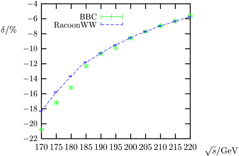
Figure 12: Relative ${\mathcal{O}}\left(\alpha\right)$ corrections to the total cross-section of ${\mathrm{e^{+}}}{\mathrm{e^{-}}}\rightarrow\nu_{\mu}\mu^{+}\tau^{-}\overline{\nu}_{\tau}$

As shown in Figure 12, both calculations agree very well above $185\,\,\mathrm{GeV}$. Below this energy the differences in the implementation of the DPA become visible, in agreement with the expected relative error of ${\mathcal{O}}\left(\Gamma_{{\scriptscriptstyle{W}}}/\Delta E\right)$. The main effect originates probably from the different treatment of the ${\mathcal{O}}(\alpha)$ ISR and the phase space. While BBC treat the complete ${\mathcal{O}}(\alpha)$ correction (including ISR) in DPA and use the on-shell phase space consistently, in RacoonWW the universal leading-log part of the ${\mathcal{O}}(\alpha)$ ISR correction is applied to the full CC11 cross-section, and the off-shell phase space is used throughout. Below about $170\,\,\mathrm{GeV}$ the DPA cannot be trusted any more for both virtual corrections and real-photon radiation, since the kinetic energy of the $W$ bosons becomes of the order of the $W$ width. The large deviations of up to $2\%$ in the energy range between $170$ and $180\,\mathrm{GeV}$ can be partially attributed to the fact that BBC treats also the leading logarithmic ISR corrections in DPA which is not done in RacoonWW. Therefore this difference cannot be viewed automatically as a theoretical uncertainty of the Monte Carlo programs.

For angular and energy distributions unavoidable differences arise from the definition of the phase-space variables in the presence of photon recombination. When defining the momenta of the $W$ bosons for angular distributions, BBC chooses to assign the photon to one of the production/decay sub-processes. If the detected photon is hard, $E_{\gamma}\gg\Gamma_{{\scriptscriptstyle{W}}}$, then this is theoretically possible. The error in the assignment is suppressed by ${\mathcal{O}}(\Gamma_{{\scriptscriptstyle{W}}}/\Delta E)$. If the detected photon is semi-soft, $E_{\gamma}\sim\Gamma_{{\scriptscriptstyle{W}}}$, then it is impossible to assign it to any of the sub-processes, but as the photon momentum is much smaller than the $W$-boson momentum, the error associated with this procedure is suppressed by the same relative ${\mathcal{O}}(\Gamma_{{\scriptscriptstyle{W}}}/\Delta E)$. The angles are then determined from the resulting $W$-momenta and the original fermion momenta. In RacoonWW, all angles are defined from the fermion momenta after eventual photon recombination. To this end, the invariant masses of the photon with each of the charged initial- or final-state fermions are calculated. If the smallest of these invariant masses is smaller than $M_{\mathrm{rec}}$ and the fermion corresponding to this invariant mass is a final-state particle, the photon is recombined with this fermion. The two different angle definitions lead to a redistribution of events in the angular distributions, which arises, in particular, from hard photon emission.

The relative corrections to the distributions in the cosines of the polar production angle, $\theta_{\mathrm{W}}=\angle({\mathrm{e}}^{+},{\mathrm{W}}^{+})$, and the decay angle, $\theta_{\mu\mathrm{W}}=\angle(\mu^{+},{\mathrm{W}}^{+})$, are compared for $\sqrt{s}=184\,\,\mathrm{GeV}$ in Figure 13.

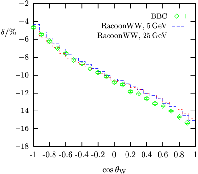
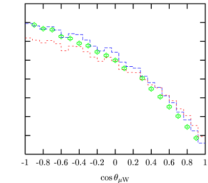
Figure 13: Relative ${\mathcal{O}}\left(\alpha\right)$ corrections to the $W$-production and decay angle distributions for ${\mathrm{e^{+}}}{\mathrm{e^{-}}}\rightarrow\nu_{\mu}\mu^{+}\tau^{-}\overline{\nu}_{\tau}$ at $\sqrt{s}=184\,\,\mathrm{GeV}$ for the two different values of $M_{\mathrm{rec}}=5\,\,\mathrm{GeV}$ and $25\,\,\mathrm{GeV}$

The results of BBC are again shown as points with error-bars. The results of RacoonWW are plotted as histograms for two different photon recombination cuts $M_{\mathrm{rec}}=5\,\,\mathrm{GeV}$ or $25\,\,\mathrm{GeV}$. The relative corrections in the two recombination schemes differ at the level of $0.5\div 1\%$, with the largest differences for large angles where the cross-section is small. The deviations between BBC and RacoonWW are somewhat larger than this and also larger than in the case of the total cross-section, but of the same order of magnitude. A repetition of the analysis at $\sqrt{s}=250\,\,\mathrm{GeV}$ has shown that the deviations at large angles grow with increasing centre-of-mass energy, since also the hard-photon redistribution effects grow with energy.

Invariant-mass distributions depend crucially on the treatment of the real photons. Since this is fundamentally different in RacoonWW and BBC, it does not make sense to compare these distributions between the two programs. Specifically, BBC define the $W$ invariant masses from the fermion momenta only (bare or muon-like) which make them sensitive to the collinear mass singularities. In RacoonWW, the photons are always recombined with the fermions (calorimetric or electron-like). The actual mass shifts crucially depend on the experimental setup. They are of the order of several $10\,\mathrm{MeV}$ and negative for the bare procedure. In the calorimetric treatment these mass shifts are reduced and can even become positive depending on the recombination procedure.

As was already mentioned earlier, the most important difference between the two approaches is the treatment of real-photon radiation. Therefore, it is important to compare distributions that are exclusive in the photon variables. As an example of such a distribution we present in Figure 14 a comparison of the photon spectrum, $E_{\gamma}\,d\sigma/dE_{\gamma}$, as a function of photon energy at the CM energy $184\,\mathrm{GeV}$.

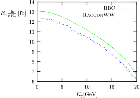
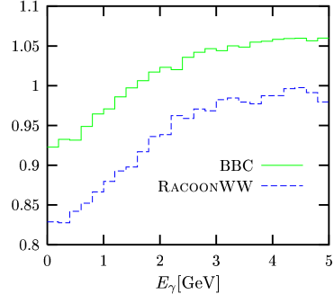
Figure 14: Photon energy spectrum, $E_{\gamma}\,d\sigma/dE_{\gamma}$, at the CM energy $184\,\mathrm{GeV}$ for the two different sets of angular cuts, as described in the text.

The spectrum is shown for two different sets of angular cuts, which restrict the angles between the photon and the beam momenta, $\angle({\mathrm{e}}^{\pm},\gamma)$, the photon and final-state lepton momenta, $\angle(\ell^{\pm},\gamma)$, and the beam and final-state lepton momenta, $\angle(\ell^{\pm},{\mathrm{e}}^{\pm})$:

1. $\angle({\mathrm{e}}^{\pm},\gamma)>1\deg$, $\angle(\ell^{\pm},\gamma)>5\deg$ and $\angle(\ell^{\pm},{\mathrm{e}}^{\pm})>10\deg$,

2. $\angle({\mathrm{e}}^{\pm},\gamma)>50\deg$, $\angle(\ell^{\pm},\gamma)>50\deg$ and $\angle(\ell^{\pm},{\mathrm{e}}^{\pm})>10\deg$.

The first set of cuts is closer to experiment, but the second suppresses the dominant contribution of ISR in the real-photonic factorizable corrections. Since the second set of cuts removes a large part of the phase space, statistics in the first case is about ten times bigger than in the second case. However, the second set of cuts renders non-factorizable and factorizable radiation of a comparable order, thus checking the former. Figure 14 reveals an agreement between the two approaches within $\sim 10\%$ for both sets of cuts, which is of the order of the naive expectation for the DPA error of ${\mathcal{O}}\left(\Gamma_{{\scriptscriptstyle{W}}}/\Delta E\right)$. Note a peculiar decrease of the photon energy spectrum at lower photon energies for the second set of cuts. It was numerically checked in the BBC approach that this decrease is due to non-factorizable contributions (interference between various stages of the process). More precisely, the non-factorizable part amounts to roughly 20% of the complete contribution and is negative for $E_{\gamma}\ll\Gamma_{{\mathrm{W}}}$; it tends to zero above $E_{\gamma}\sim\Gamma_{{\mathrm{W}}}$.

Comparison of RacoonWW and YFSWW3 results

Authors

RacoonWW	A.Denner, S.Dittmaier, M.Roth and D.Wackeroth
YFSWW3	S. Jadach, W. Placzek, M. Skrzypek, B. Ward and Z. Was

In this section we compare results obtained with the Monte Carlo generators RacoonWW [22, 20] and YFSWW3 [76]. The numerical comparison has been done for the LEP 2 input parameter set. This comparison is restricted to the CC03 contributions for ${\mathrm{e^{+}}}{\mathrm{e^{-}}}\rightarrow{\mathrm{W}}{\mathrm{W}}\rightarrow 4f$, i.e. background diagrams have been omitted.

First we recall that RacoonWW contains the complete electroweak ${\mathcal{O}}(\alpha)$ corrections to ${\mathrm{e^{+}}}{\mathrm{e^{-}}}\rightarrow{\mathrm{W}}{\mathrm{W}}\rightarrow 4f(+\gamma)$ within the DPA, including the non-factorizable corrections and $W$-spin correlations. Real-photon emission is based on the full ${\mathrm{e^{+}}}{\mathrm{e^{-}}}\rightarrow 4f\gamma$ matrix element (of the CC11 class), and ISR beyond ${\mathcal{O}}(\alpha)$ is treated in the structure-function approach with soft-photon exponentiation and leading-logarithmic contributions in ${\mathcal{O}}(\alpha^{3})$. To be more precise, for $4f$ and $4f\gamma$ (with a hard non-collinear $\gamma$) at tree level all final states are supported, i.e. also Mix43, i.e. $\overline{u}d\overline{d}u$. If, however, soft and collinear photons are allowed, the virtual correction to $e^{+}e^{-}\rightarrow WW\rightarrow 4{\rm f}$ is required. In this case, RacoonWW takes photon radiation from the CC11 class into account. The singular Coulomb correction is included with its full off-shell behaviour.QCD corrections are taken into account by the naive QCD factors $(1+\alpha_{\mathrm{s}}/\pi)$ for hadronically decaying $W$ bosons.

In YFSWW3 the exact ${\mathcal{O}}(\alpha)$ electroweak corrections to ${{\mathrm{e}}^{+}{\mathrm{e}}^{-}\rightarrow{\mathrm{W}}^{+}{\mathrm{W}}^{-}}$ are implemented together with YFS exponentiation of the corresponding soft-photon effects for the production process as defined in the DPA, which is equivalent to the LPA as defined in Ref. [77] for this process. ISR beyond ${\mathcal{O}}(\alpha)$ is taken into account up to ${\mathcal{O}}(\alpha^{3})$ in leading-logarithmic approximation. The full off-shell behaviour of the singular Coulomb correction is included. The corrections to the $W$ decay, including naive QCD corrections, are implemented by using the corrected branching ratios. In this way, the total cross-section receives the full ${\mathcal{O}}(\alpha)$ corrections in DPA. Taking this cross section as normalization, final-state radiation with up to two photons is generated by PHOTOS, which is based on a leading-logarithmic (LL) approximation in which finite $p_{\mathrm{T}}$ effects are taken into account in such a way that the soft limit of the respective exact ${\mathcal{O}}\left(\alpha\right)$ $p_{\mathrm{T}}$ spectrum is reproduced.

For observables where the decay of the $W$ bosons and their off-shellness are integrated out, the expected differences between the two calculations are of the order of the accuracy of the DPA, i.e. of the relative order ${\mathcal{O}}\left(\alpha\Gamma_{{\mathrm{W}}}/\Delta E\right)$, modulo possible enhancement factors. Here $\Delta E$ is a typical energy scale for the considered observable, i.e. $\Delta E\sim\sqrt{s}-2M_{\mathrm{W}}$ for the total cross-section near the $W$-pair production threshold. For observables that depend on the momenta of the decay products larger differences can be expected. This holds, in particular, for observables involving a real photon. While such observables are based on the full lowest-order matrix element for ${\mathrm{e^{+}}}{\mathrm{e^{-}}}\rightarrow 4f\gamma$ in RacoonWW, in YFSWW3 the multi-photon radiation in the $WW$ production (within the YFS scheme) is combined with ${\mathcal{O}}(\alpha^{2})$ LL radiation in $W$-decays (done by PHOTOS), i.e. the real photon radiation is treated in DPA and some finite ${\mathcal{O}}(\alpha)$ terms from FSR are neglected, but the treatment of the leading logarithms goes beyond strict ${\mathcal{O}}(\alpha)$.

For the total cross-section, the differences between the two approaches should be of the naively expected DPA accuracy, i.e. below 0.5% for $\sqrt{s}>180\,\,\mathrm{GeV}$. In Table 7 we compare the results from both generators for the total cross-section without any cuts. The best numbers correspond to the inclusion of all corrections implemented in the programs. Independently of the channel both programs differ by $0.2\div 0.3\%$, which is of the order of the intrinsic ambiguity of any DPA implementation, i.e. the numbers are consistent with each other.

no cuts		$\sigma_{\mathrm{tot}}[\mathrm{fb}]$
final state	program	Born	best
	YFSWW3	219.770(23)	199.995(62)
$\nu_{\mu}\mu^{+}\tau^{-}\bar{\nu}_{\tau}$	RacoonWW	219.836(40)	199.551(46)
	(Y–R)/Y	$-0.03(2)$%	0.22(4)%
	YFSWW3	659.64(07)	622.71(19)
${\mathrm{u}}\bar{\mathrm{d}}\mu^{-}\bar{\nu}_{\mu}$	RacoonWW	659.51(12)	621.06(14)
	(Y–R)/Y	$0.02(2)$%	0.27(4)%
	YFSWW3	1978.18(21)	1937.40(61)
${\mathrm{u}}\bar{\mathrm{d}}{\mathrm{s}}\bar{\mathrm{c}}$	RacoonWW	1978.53(36)	1932.20(44)
	(Y–R)/Y	$-0.02(2)$%	0.27(4)%

Table 7: Total cross-sections for CC03 from RacoonWW and YFSWW3 at $\sqrt{s}=200\,\,\mathrm{GeV}$ without cuts. The numbers in parentheses are statistical errors corresponding to the last digits.

The results of YFSWW3 presented here differ from the ones presented at the winter conferences, where still a difference of $0.7\%$ between the programs was reported. The main point is that the results in Table 7 are obtained with version 1.14 whereas those presented at the winter conferences were obtained with version 1.13. Version 1.14, which has benefitted from the detailed comparison between the RacoonWW and YFSWW3 virtual corrections, represents, according to renormalization group improved YFS theory [78], an improved re-summation of the higher order corrections as compared to version 1.13. We stress that we (the RacoonWW and YFSWW3 groups) have also checked that, when we use the same couplings, our ${\mathcal{O}}\left(\alpha\right)$ virtual plus soft corrections in the W-pair production building block agree differentially at the sub-per mille level and agree for the total cross section at $<0.01\%$. This is an important cross check on both programs. However, as a by-product of this detailed comparison, we have realized that the $G_{{\scriptscriptstyle{F}}}$ scheme of Refs. [79] has only the IR divergent part of the virtual photonic corrections with coupling $\alpha(0)$ whereas the renormalization group equation implies that any photon of 4-momentum $q$ should couple completely with $\alpha(0)$ when $q^{2}\rightarrow 0$, where $\alpha(q^{2})$ is the running renormalized QED coupling. In version 1.14 of YFSWW3, we have made this improvement as implied by the renormalization group equation [78]. The generic size of the resulting shift in the YFSWW3 prediction can be understood by isolating the well-known soft plus virtual LL ISR correction to the process at hand, which has in ${\mathcal{O}}\left(\alpha\right)$ the expression [79]

$$\delta^{v+s}_{ISR,LL}=\beta\ln k_{0}+\frac{\alpha}{\pi}\left(\frac{3}{2}L+\frac{\pi^{2}}{3}-2\right),$$ (61)

where $\beta\equiv\frac{2\alpha}{\pi}(L-1)$, $L=\ln(s/m_{e}^{2})$, and $k_{0}$ is a dummy soft cut-off which cancels out of the cross section as usual. In the $G_{{\scriptscriptstyle{F}}}$ scheme of Refs. [79] which is used in YFSWW3-1.13, only the part $\beta\ln k_{0}+(\alpha/\pi)(\pi^{2}/3)$ of $\delta^{v+s}_{ISR,LL}$ has the coupling $\alpha(0)$ and the remaining part of $\delta^{\rm v+s}_{ISR,LL}$ has the coupling $\alpha_{G_{{\scriptscriptstyle{F}}}}\cong\alpha(0)/(1-0.0371)$. The renormalization group improved YFS theory implies, however, that $\alpha(0)$ should be used for all the terms in $\delta^{v+s}_{ISR,LL}$. This is done in YFSWW3-1.14 and results in the normalization shift $\left((\alpha(0)-\alpha_{G_{{\scriptscriptstyle{F}}}})/\pi\right)(1.5L-2)$, which at 200GeV is $\sim-0.33\%$. This explains most of the change in the normalization of YFSWW3-1.14 vs that of YFSWW3-1.13. Moreover, it does not contradict the expected total precision tag of either version of YFSWW3 at their respective stages of testing. We stress that, according to the renormalization group equation, version 1.14 is an improvement over version 1.13 – it better represents the true effect of the respective higher order corrections. More details of the actual scheme of renormalization and re-summation used in YFSWW3-1.14 will appear elsewhere [59].

In RacoonWW, the coupling $\alpha(0)$ is used everywhere in the relative ${\mathcal{O}}\left(\alpha\right)$ corrections, even in the $G_{{\scriptscriptstyle{F}}}$ scheme, in order to include the appropriate coupling for the (dominant) photonic corrections. A switch in YFSWW3-1.14 to this scheme shifts the maximal differences between the programs to $0.34\%$, somewhat larger than the $0.27\%$ shown. This confirms the expectation that the effects of unknown higher-order corrections are at the level of $0.1\%$.

It should be noted that the results in Table 7 lie by $2\div 3\%$ below the LL-type predictions given by GENTLE [68] (see also Section 4). As stated above, however, this consideration only applies to GENTLE in some special setup. The disagreement with all other codes active in the ‘95 workshop [5] is within $1.5\%$. The fact that two independent Monte Carlo calculations with physical precision at the level of ${\mathcal{O}}(\frac{\alpha}{\pi}\frac{\Gamma_{{\scriptscriptstyle{W}}}}{M_{{}_{W}}})$ now agree to $0.2\div 0.3\%$ at $200\,$GeV for this total cross section is truly an important improvement over the situation in the ’95 workshop [5].

In the following we consider observables obtained with the cut and photon recombination procedure as given in the description of numerical results of RacoonWW in Sect. 4.1. We again consider the cases of a tight recombination cut $M_{\mathrm{rec}}=5\,\,\mathrm{GeV}$ (bare) and of a loose recombination cut $M_{\mathrm{rec}}=25\,\,\mathrm{GeV}$ (calo).

Table 8 shows the analogous cross-sections to Table 7 but now with the described bare cuts applied. The difference of $0.2\div 0.3\%$ between the two compared programs does not change by the applied cuts. When turning from bare to calo cuts the results for the cross-sections do not change significantly; of course, the lowest-order results do not change at all.

In the following relative corrections to various distributions for the semi-leptonic channel ${\mathrm{e^{+}}}{\mathrm{e^{-}}}\rightarrow{\mathrm{u}}\bar{\mathrm{d}}\mu^{-}\overline{\nu}_{\mu}$ are compared at $\sqrt{s}=200\,\,\mathrm{GeV}$. All these distributions have been calculated using the above set of separation and recombination cuts.

The corrections to the cosine of the production angle for the ${\mathrm{W^{+}}}$ and ${\mathrm{W^{-}}}$ bosons are shown in Figures 15 and 16, respectively, for the bare (left) and the calo (right) recombination schemes. The distributions are compatible with each other to better than $1\%$. The largest differences are of the order of $1\%$ and appear in general for large scattering angles.

Figure 15: Distribution in the cosine of the ${\mathrm{W^{+}}}$ production angle with respect to the ${\mathrm{e^{+}}}$ beam for the bare (left) and calo (right) setup at $\sqrt{s}=200\,\,\mathrm{GeV}$ for ${\mathrm{u}}\bar{\mathrm{d}}\mu^{-}\overline{\nu}_{\mu}$ final state.

Figure 16: Distribution in the cosine of the ${\mathrm{W^{-}}}$ production angle with respect to the ${\mathrm{e^{-}}}$ beam for the bare (left) and calo (right) setup at $\sqrt{s}=200\,\,\mathrm{GeV}$ for ${\mathrm{u}}\bar{\mathrm{d}}\mu^{-}\overline{\nu}_{\mu}$ final state.

with bare cuts		$\sigma_{\mathrm{tot}}[\mathrm{fb}]$
final state	program	Born	best
	YFSWW3	210.918(23)	192.147(63)
$\nu_{\mu}\mu^{+}\tau^{-}\bar{\nu}_{\tau}$	RacoonWW	211.034(39)	191.686(46)
	(Y–R)/Y	$-0.05(2)$%	0.24(4)%
	YFSWW3	627.18(07)	592.68(19)
${\mathrm{u}}\bar{\mathrm{d}}\mu^{-}\bar{\nu}_{\mu}$	RacoonWW	627.22(12)	590.94(14)
	(Y–R)/Y	$-0.01(2)$%	0.29(4)%
	YFSWW3	1863.40(21)	1826.80(62)
${\mathrm{u}}\bar{\mathrm{d}}{\mathrm{s}}\bar{\mathrm{c}}$	RacoonWW	1864.28(35)	1821.16(43)
	(Y–R)/Y	$-0.05(2)$%	0.31(4)%

Table 8: Total cross-sections for CC03 from YFSWW3 and RacoonWW at $\sqrt{s}=200\,\mathrm{GeV}$ with bare cuts (see text). The numbers in parentheses are statistical errors corresponding to the last digits.

The corrections to the invariant mass distributions for the ${\mathrm{W^{+}}}$ and ${\mathrm{W^{-}}}$ bosons are shown in Figures 17 and 18 for the bare (left) and the calo (right) recombination scheme. The distributions are statistically compatible with each other everywhere and agree within 1%. It should be noted that the distortion of the distributions is mainly due to radiation off the final state and the $W$ bosons. It may seem remarkable that the LL approach of PHOTOS properly accounts for these distortion effects. But one should remember that PHOTOS was fine-tuned to describe the exact ${\mathcal{O}}\left(\alpha^{1}\right)$ FSR for the radiative $Z$ and $\tau$ decays, like $Z\rightarrow\mu^{-}\mu^{+}(\gamma)$ and $\tau\rightarrow\mu\nu\bar{\nu}(\gamma)$. PHOTOS was also cross-checked against the exact matrix element for the $W\rightarrow\mu\nu\gamma$ process.

Figs. 19, 20, and Fig. 21 show the distributions in the photon energy $E_{\gamma}$, in the cosine of the polar angle of the photon (w.r.t. the ${\mathrm{e^{+}}}$ axis), and in the angle between the photon and the nearest final-state charged fermion from the two programs and in the two recombination schemes.

The differences are of the order of $15\div 20\%$. Differences of this order may be expected, since photonic observables are no corrections anymore, but belong to the class of ${\mathrm{e^{+}}}{\mathrm{e^{-}}}\rightarrow 4f\gamma$ processes, since ${\mathrm{e^{+}}}{\mathrm{e^{-}}}\rightarrow 4f$ does not contribute here. Whether or not the observed differences are consistent with the differences in the treatments of the real photon emission in the two programs is under investigation.

Figure 17: Distribution in the ${\mathrm{W^{+}}}$ invariant mass for bare (left) and calo (right) setup at $\sqrt{s}=200\,\,\mathrm{GeV}$ for ${\mathrm{u}}\bar{\mathrm{d}}\mu^{-}\overline{\nu}_{\mu}$ final state.

Figure 18: Distribution in the ${\mathrm{W^{-}}}$ invariant mass for bare (left) and calo (right) setup, $\sqrt{s}=200\,\,\mathrm{GeV}$, for ${\mathrm{u}}\bar{\mathrm{d}}\mu^{-}\overline{\nu}_{\mu}$ final state.

Figure 19: Distribution in photon energy $E_{\gamma}$ (from YFSWW3 $E_{\gamma}$ of the hardest photon) for the bare (left) and calo (right) setup at $\sqrt{s}=200\,\,\mathrm{GeV}$ for ${\mathrm{u}}\bar{\mathrm{d}}\mu^{-}\overline{\nu}_{\mu}$ final state.

Figure 20: Distribution in the cosine of the polar angle of the (in YFSWW3 hardest) photon w.r.t. the ${\mathrm{e^{+}}}$ beam for bare (left) and calo (right) setup at $\sqrt{s}=200\,\,\mathrm{GeV}$ for ${\mathrm{u}}\bar{\mathrm{d}}\mu^{-}\overline{\nu}_{\mu}$ final state.

Figure 21: Distribution in the angle between the (for YFSWW3 hardest) photon and the nearest final-state charged fermion for bare (left) and calo (right) setup at $\sqrt{s}=200\,\,\mathrm{GeV}$

4.2 Internal estimate of theoretical uncertainty for CC03

Here we give a quantitative statement on the theoretical precision for DPA-approximation.

Estimating the theoretical uncertainty of the DPA with RacoonWW

Authors

A.Denner, S. Dittmaier, M. Roth and D.Wackeroth

All existing calculations of electroweak corrections to ${\mathrm{e^{+}}}{\mathrm{e^{-}}}\rightarrow{\mathrm{W}}{\mathrm{W}}\rightarrow 4f$ are based on DPA. A naive estimate of the accuracy of this approach yields $(\alpha/\pi)\times\ln(\ldots)\times\Gamma_{{\mathrm{W}}}/M_{\mathrm{W}}$, where $\Gamma_{{\mathrm{W}}}/M_{\mathrm{W}}$ is the generic accuracy of the DPA, $\alpha/\pi$ results from considering one-loop corrections, and $\ln(\ldots)$ represents leading logarithms or other possible enhancement factors in the corrections. This naive estimate suggests that the DPA has an uncertainty of some $0.1\%$. Note, however, that this estimate can fail whenever small scales become relevant. In particular near the $W$-pair threshold, the estimate should be replaced by $(\alpha/\pi)\times\ln(\ldots)\times\Gamma_{{\mathrm{W}}}/(\sqrt{s}-2M_{\mathrm{W}})$.

In order to investigate the accuracy of the DPA quantitatively, a number of tests have been performed with RacoonWW. The implementation of the DPA has been modified within the formal level of $\alpha\Gamma_{\mathrm{W}}/M_{\mathrm{W}}$, and the obtained results have been compared. Note that in RacoonWW only the virtual corrections are treated in DPA, while real photon emission is based on the full ${\mathrm{e^{+}}}{\mathrm{e^{-}}}\rightarrow 4f\gamma$ matrix element with the exact five-particle phase space. Thus, only the $2\rightarrow 4$ part is effected by the following modifications. Specifically, three types of uncertainties have been considered (see Ref. [22] for details):

• Different on-shell projections:
  In order to define a DPA one has to specify a projection of the physical momenta to a set of momenta for on-shell $W$-pair production and decay. This can be done in an obvious way by fixing the direction of one of the $\mathrm{W}$ bosons and of one of the final-state fermions originating from either $\mathrm{W}$ boson in the CM frame of the incoming ${\mathrm{e^{+}}}{\mathrm{e^{-}}}$ pair. The default in RacoonWW is to fix the directions of the momenta of the fermions (not of the anti-fermions) resulting from the ${\mathrm{W^{+}}}$ and ${\mathrm{W^{-}}}$ decays (def). A different projection is obtained by fixing the direction of the anti-fermion from the ${\mathrm{W^{+}}}$ decay (proj) instead of the fermion direction.

• Treatment of soft photons:
  In RacoonWW, the virtual photon contribution is treated in DPA, while real photon radiation is fully taken into account. These two contributions have to be matched in such a way that IR and mass singularities cancel. This requirement only fixes the universal, singular parts, but leaves some freedom to treat non-universal, non-singular contributions in DPA or not. For instance, in the branch of RacoonWW that employs the subtraction method of Ref. [41], the endpoint contributions of the subtraction functions are calculated in DPA and added to the virtual photon contribution as default. As an option, RacoonWW allows to treat also the universal (IR-sensitive) part of the virtual photon contribution off-shell by extracting an U(1)-invariant factor à la YFS [80] from the virtual photon contribution and adding it to the real photon contribution, i.e. this soft+virtual part of the photonic correction is treated off shell (eik). The two described treatments only differ by terms of the form $(\alpha/\pi)\times\pi^{2}\times{\mathcal{O}}\left(1\right)$ which are either multiplied with the DPA (def) or with the full off-shell Born cross-sections (eik).

• On-shell versus off-shell Coulomb singularity:
  The Coulomb singularity is (up to higher orders) fully contained in the virtual ${\mathcal{O}}\left(\alpha\right)$ correction in DPA. Performing the on-shell projection to the full virtual correction leads to the on-shell Coulomb singularity. However, since the Coulomb singularity is an important correction in the LEP 2 energy range and is also known beyond DPA, RacoonWW includes this extra off-shell Coulomb correction as default. Switching the extra off-shell parts of the Coulomb correction off (Coul), yields an effect of the order of the accuracy of the DPA.

In the following table and figures the total cross-section and various distributions have been compared for the different versions of the DPA defined above. The results have been obtained using the LEP 2 input parameter set and the set of separation and recombination cuts as given in the description of numerical results of RacoonWW in Sect. 4.1. The recombination cut is chosen to be $M_{\mathrm{rec}}=25\,\,\mathrm{GeV}$. As default, we take the RacoonWW results (best-with-4f-Born) of Sect. 4 for the process ${\mathrm{e^{+}}}{\mathrm{e^{-}}}\rightarrow{\mathrm{u}}\bar{\mathrm{d}}\mu^{-}\overline{\nu}_{\mu}(\gamma)$ at $\sqrt{s}=200\,\,\mathrm{GeV}$, which are based on the above input. The only differences are that the naive QCD factors and ISR corrections beyond ${\mathcal{O}}\left(\alpha\right)$ are not included in the results of this section. The results for the total cross-section are shown in Table 9.

def proj eik Coul $\sigma/\mathrm{pb}$ 570.53(46) 570.37(46) 570.47(46) 571.28(46) $\delta/\%$ 0 $-0.03$ $-0.01$ 0.13

Table 9: RacoonWW predictions for the total cross-section of ${\mathrm{e^{+}}}{\mathrm{e^{-}}}\rightarrow{\mathrm{u}}\bar{}{\mathrm{d}}\mu^{-}\overline{\nu}_{\mu}(\gamma)$ at $\sqrt{s}=200\,\,\mathrm{GeV}$ in various versions of the DPA and relative differences $\delta=\sigma/\sigma_{\mathrm{def}}-1$

Note that these cross-sections are calculated with the above cuts. We find relative differences at the level of $0.1\%$. As expected, the prediction that is based on the on-shell Coulomb correction is somewhat higher than the exact off-shell treatment, since off-shell effects screen the positive Coulomb singularity. The results in Table 9 have been obtained using phase-space slicing for the treatment of the IR and collinear singularities. If the subtraction method is used instead, the resulting cross-section is about 0.01% smaller.

In Figures 22 and 23 we show the differences of the proj, eik, and Coul modifications to the default version of the DPA for some distributions. For the distribution in the cosine of the W-production angle $\theta_{{\mathrm{W}}^{+}}$ and in the W-decay angle $\theta_{{\mathrm{W}}^{-}\mu^{-}}$ (see Figure 22) the relative differences are of the order of $0.1\div 0.2\%$ for all angles, which is of the expected order for the intrinsic DPA uncertainty.

Figure 22: Theoretical uncertainty within the DPA for distributions in the W-production and W-decay angles for ${\mathrm{e^{+}}}{\mathrm{e^{-}}}\rightarrow{\mathrm{u}}\bar{}{\mathrm{d}}\mu^{-}\overline{\nu}_{\mu}(\gamma)$ at $\sqrt{s}=200\,\,\mathrm{GeV}$

Figure 23: Theoretical uncertainty within the DPA for distributions in the $\mu$ energy and in the ${\mathrm{u}}\bar{}{\mathrm{d}}$ invariant mass for ${\mathrm{e^{+}}}{\mathrm{e^{-}}}\rightarrow{\mathrm{u}}\bar{}{\mathrm{d}}\mu^{-}\overline{\nu}_{\mu}(\gamma)$ at $\sqrt{s}=200\,\,\mathrm{GeV}$

For the $\mu$-energy distribution, shown in the l.h.s. of Figure 23, the differences are typically of the same order, as long as $E_{\mu}$ is in the range for $W$-pair production, which is $20.2\,\,\mathrm{GeV}<E_{\mu}<79.8\,\,\mathrm{GeV}$ at $\sqrt{s}=200\,\,\mathrm{GeV}$. Outside this region, the four-fermion process is not dominated by the $W$-pair diagrams, and the DPA is not reliable anymore, which is also indicated by large intrinsic ambiguities. The r.h.s. of Figure 23 shows the DPA uncertainties for the ${\mathrm{u}}\bar{\mathrm{d}}$ invariant-mass distribution. Within a window of $2\Gamma_{\mathrm{W}}$ around the W resonance the relative differences between the considered modifications are also at the level of $0.1\div 0.2\%$. The differences grow with the distance from the resonance point.

The discussed results illustrate that the intrinsic ambiguities of the DPA, as applied in RacoonWW, are at the level of a few per mil, whenever resonant $W$-pair production dominates the considered observable.

Estimating the theoretical uncertainty of the DPA with YFSWW3-KoralW

The accuracy of the combined result from YFSWW3 1.13 and our all 4-fermion process MC KoralW 1.42  [81] as presented in Ref. [59] is expected to be below $0.5\%$ for the total cross-section when all tests are finished. These tests are currently in progress.

4.3 Summary and conclusions

In this Section we have compared different theoretical predictions for the CC03 cross-section that have been used to analyze the data in terms of all $W$-pair final states, $4q(qqqq)$ and non-$4q(qq{\rm l}\nu,{\rm l}\nu{\rm l}\nu)$. The major achievement in this area is represented by inclusion of radiative corrections in DPA for the $WW$ cross-section.

Data are collected from $161\,$GeV up to $210\,$GeV. One should remember that below some threshold ($\approx 170\,\,\mathrm{GeV}$) the DPA cannot be trusted any more for both virtual corrections and real-photon radiation, since the kinetic energy of the $W$ bosons becomes of the order of the $W$ width. RacoonWW has shown that the intrinsic ambiguities of its implementation of the DPA are at the level of a few per mille.

For the total CC03 cross-section, the differences between RacoonWW and YFSWW should be of the naively expected DPA accuracy, i.e. below 0.5% for $\sqrt{s}>180\,\,\mathrm{GeV}$. And, indeed, independently of the channel, the two MC differ by $0.2\div 0.3\%$ in the results presented herein and this increases to 0.4% if uncertainties from unknown higher-order corrections are taken into account. Note that, with bare cuts applied, the difference of $0.2\div 0.3\%$ shown here between the two compared programs does not change.

The corrections to the distribution in the cosine of the production angle for the ${\mathrm{W^{+}}}$ and ${\mathrm{W^{-}}}$ bosons have also been analyzed for the bare and the calo recombination algorithms. They are compatible with each other at a level below 1%. Although compatible with the statistical accuracy, the deviations seem to become somewhat larger for large scattering angles. The corrections to the invariant mass distributions for the ${\mathrm{W^{+}}}$ and ${\mathrm{W^{-}}}$ bosons, again with bare and calo recombinations are statistically compatible between the two Monte Carlo programs everywhere and agree within 1%.

Another comparison, shown in Figure 12, indicates that RacoonWW and BBC calculations agree very well for the total $W$-pair production cross-section above $185\,\,\mathrm{GeV}$. Below this energy the differences in the implementation of the DPA become visible, in agreement with the expected relative error of ${\mathcal{O}}\left(\alpha/\pi\times\Gamma_{{\scriptscriptstyle{W}}}/\Delta E\right)$. However, for angular and energy distributions unavoidable differences at the level of $1\div 2\%$ arise between the two predictions, as a consequence of the definition of the phase-space variables in the presence of photon recombination. Although the BBC-calculation has not been implemented in a MonteCarlo it can be used for obtaining a relative ${\mathcal{O}}\left(\alpha\right)$ correction factor where one has an estimated internal accuracy ranging from $1.5\%$ at lower energies to $0.3\%$ at $210\,$GeV.

In conclusion, from the direct comparisons of RacoonWW and YFSWW3, supported by BBC, we can estimate an overall theoretical uncertainty of the current predictions for the total $WW$ cross-section at $0.4\%$ at $200\,\,\,\mathrm{GeV}$. The $0.4\%$ precision tag is an important conclusion of this Workshop.

For other energies no complete investigations of the theoretical uncertainty have been performed. However, based on the error estimate of $0.4\%$ for $200\,\mathrm{GeV}$, the intrinsic uncertainty of the DPA of $0.2\%$ at $200\,\mathrm{GeV}$ and the generic energy dependence of this uncertainty given by $\Gamma_{{}_{W}}/(E_{\rm CMS}-2M_{\mathrm{W}})$ we estimate an uncertainty of the predictions of RacoonWW and YFSWW3 of $0.5\%$ for $180\,\mathrm{GeV}$ and $0.7\%$ for $170\,\mathrm{GeV}$. This could be somewhat further reduced, if the sources of the differences between the different programs are found.

Results for the $WW$ cross-section at ${\mathcal{O}}\left(\alpha\right)$ are also available from GRACE but a comparison with the other codes is not yet at the level of those already presented where a considerable amount of time was invested to try to understand differences towards a safe estimate of theoretical uncertainty.

5 Four fermions plus a visible photon

The class of processes that are investigated at LEP 2 are $e^{+}e^{-}\rightarrow W^{+}W^{-}\rightarrow 4\,$f, single-$W$ production, $Z$-boson-pair production, single-$Z$ production. LEP 2 and also future linear colliders will allow us to study a new class of processes, $e^{+}e^{-}\rightarrow 4{\rm f}+\gamma$.

The physical interest of the latter is twofold. They can be used to obtain informations on the quartic gauge-boson couplings and include the production processes of three gauge-bosons, $W^{+}W^{-}\gamma$, $ZZ\gamma$ and $Z\gamma\gamma$. In this case the photon is visible by definition and we term the corresponding process radiative, i.e. we consider as radiative events those events with photons where at least one photon passes the experimental photon requirements, for instance $E_{\gamma}>1\,$GeV, $\cos\theta_{\gamma}<0.985(0.997)$ and $\theta_{f-\gamma}>5^{\circ}$.

Note that for all final states, the invariant mass needs a more precise definition in case radiative photons are present in the event. From a calculational point of view, there is always a minimal invariant mass (energy and separation angle) below which photons are not resolved. Thus we need to specify fermion-photon invariant mass or fermion-photon energies and separation angles, below which the the photon are combined with the fermion and above which the photons are not included in the mass calculation. A bare mass would set these cuts rather tight, excluding photons from the $f\overline{f}$ mass, a calo mass would set the separation cuts looser. Theorists like cuts on $M(\gamma-{\rm nearestf})$. Experimentalists like cuts on energies and angles. In the following we list both TH(eory)-cuts and EXP(erimental)-cuts.

TH cuts

:

• $M(\overline{f}f+(\gamma))$ including photons if $M(f+\gamma)<5\,$GeV,

• $M(\overline{f}f+(\gamma))$ including photons if $M(f+\gamma)<25\,$GeV.

EXP-cuts

:

• : $M(\overline{f}_{1}f_{2}+(\gamma))$, photons less than 1 GeV or less than $1^{\circ}$ away from $f_{1}$ or $f_{2}$ are included;

• : $M(\overline{l}_{1}l_{2}+(\gamma))$, photons less than 1 GeV or less than $10^{\circ}$ away from charged leptons are included,
  $M(\overline{q}_{1}q_{2}+(\gamma))$, photons less than 1 GeV or less than $25^{\circ}$ away from either quark $q_{1},q_{2}$ are included, which takes at least the major difference between fermions - quarks versus leptons - into account.

These definitions serve for benchmarking distributions, not so much to mimic an actual experimental strategy, which is of course fermion dependent. In other words this is an approximation to the experimental side: if the fermion is a muon, even $0^{\circ}$ opening angles can be separated experimentally. In addition, for identified photons one still may or may not choose to recombine the photon with the fermion.

Furthermore, $e^{+}e^{-}\rightarrow 4{\rm f}+\gamma$ is an important building block for the radiative corrections to the Born process $e^{+}e^{-}\rightarrow 4\,$f, hence non-radiative events are those with no photon or only photons below the minimal photon requirements. In case of non-radiative events, this amounts to adding up virtual and soft radiative corrections. The effect of ${\mathcal{O}}\left(\alpha\right)$ QED corrections very often amounts to several percent, mostly originating from collinear photon radiation off highly energetic particles and from virtual photon exchange. For initial state radiation, for instance, we have three types of corrections, a) ${\mathcal{O}}\left(\alpha/\pi\,\ln(m_{e}/Q)\right)$ with $Q\gg m_{e}$ being the typical scale at which the process occur, b) ${\mathcal{O}}\left(\alpha/\pi\right)$ from hard photons that must, nevertheless, be included for a $1\%$ precision tag, c) leading ${\mathcal{O}}\left(\alpha^{2}\right)$, or higher corrections that becomes relevant for a precision tag below the $1\%$ thresholds.

Owing to the fact that a theoretical prediction with a typical accuracy of some fraction of a percent must include all QED corrections, we face the complexity of it. Handling the singularities of the squared matrix element represents a formidable task; in any bremsstrahlung process the integrand blows up for arbitrary small photon energies and similar problems arise from collinear emission off the charged particles.

A general comment about this section is that some of the programs, but not all, implement $4{\rm f}+\gamma$ at the level of (exact) matrix elements. Few programs have only an effective treatment of photons via structure functions, with or without $p_{t}$. Furthermore we also have to distinguish between massless vs. massive calculations.

5.1 Description of the programs and their results

$4{\rm f}+\gamma$ with RacoonWW

Authors

A.Denner, S.Dittmaier, M.Roth and D.Wackeroth

General description

The program RacoonWW [22] evaluates cross-sections and differential distributions for the reactions ${\mathrm{e^{+}}}{\mathrm{e^{-}}}\rightarrow 4{\rm f}$ and ${\mathrm{e^{+}}}{\mathrm{e^{-}}}\rightarrow 4{\rm f}+\gamma$ for all four-fermion final states. The long write-up has already been presented in Sect. 4.1, so that we only stress the features that are peculiar to $4{\rm f}+\gamma$ production with a separated hard photon. The calculation is based on full $4{\rm f}+\gamma$ matrix elements for all final possible states. Since fermion masses are neglected, lower cuts on the invariant mass of ${\rm f}\bar{\rm f}$ pairs and on ${\mathrm{e}}^{\pm}$ emission angles have to be imposed, in addition to the angular and energy cuts for the hard photon. RacoonWW supports different ways to treat finite gauge-boson widths (fixed and running widths, complex-mass scheme) and allows to select subsets of graphs ($VV\gamma$ signal diagrams, QCD background). Detailed numerical results on $4{\rm f}+\gamma$ production with RacoonWW can be found in Ref. [18] and in Sect. 5.2.

$4{\rm f}+\gamma$ with PHEGAS/HELAC

Author

C. G. Papadopoulos

This section refers to a novel Monte Carlo program that is capable to deal with any tree-order process involving any particle and interaction described by the Standard Model, including QCD.

The program consists of two modules:

1. HELAC which is a matrix element computation-tool [60] based on Dyson-Schwinger equations, and

2. PHEGAS an automatic phase-space generator [61] capable to simulate all peaking structures of the amplitude.

The over all code is using a Monte Carlo integration based on multichannel optimization [62].

HELAC

The matrix element is evaluated using a recursive approach based on Dyson-Schwinger equations. The computational cost exhibits an exponential growth ($\simeq 3^{n}$) as a function of the number of external particles ($n$) which for multi-particle processes results to a very important increase in the efficiency as compared with the traditional Feynman-graph approach whose computational cost grows factorially ($\simeq n!$). In order to optimize code’s efficiency the computational strategy consists of two phases. In the first phase a solution to the recursive equations is established in terms of an integer array containing all relevant information for the process under consideration. This is the initialization phase and is performed once at the beginning of the execution of the program. In the second phase, using the already generated information, the actual computation is performed resulting to the numerical evaluation of the amplitude for each specific phase-space point provided.

In order to consistently describe unstable particles the fixed width as well as the complex width schemes have been included. ISR and running couplings are also an option and work is in progress to implement higher order corrections within the approach of reference [16].

In order to deal with numerical stability problems, besides the double precision, a quadruple as well as a multi-precision [63] version is available. This makes HELAC able to deal with processes exhibiting strong collinear singularities, like $e^{-}e^{+}\rightarrow e^{-}e^{+}\mu^{-}\mu^{+}$ at zero scattering angles. Moreover all particle masses and vertices of the Standard Model, including QCD, in both the Feynman and unitary gauges are incorporated.

PHEGAS

Although several matrix element computational tools were available in the past that can deal with arbitrary processes, to the one or to the other extent [64], phase-space generators were always developed according to a specific process or a class of processes [65]. PHEGAS is a phase space generator that incorporates in an automatic way all possible kinematical mappings for any given process, using the relevant information provided by HELAC. To this end each Feynman graph contributing to the process under consideration gives rise to a kinematical mapping. The integration is performed via a Monte Carlo multichannel approach and during the computation, weight optimization selects automatically those kinematical mappings that are relevant for the process under consideration.

As a first highly non-trivial test PHEGAS/HELAC has been used to produce results for four-fermion plus a visible photon within the current study. Nevertheless, it is worthwhile to emphasize that PHEGAS/HELAC is able to deal with any process involving any Standard Model particle and is by no means restricted to $e^{+}e^{-}\rightarrow\mbox{4 f}+\gamma$ reactions. A detailed presentation of the code, the implemented algorithms as well as the incorporated physics effects will be available in the near future [61].

$4{\rm f}+\gamma$ with WRAP

Authors

G. Montagna, M. Moretti, O. Nicrosini, M. Osmo and F. Piccinini

Description of the Method.

Contributions of the Pavia/ALPHA group to the subject of four fermions plus gamma final states are summarized.

Hard-scattering matrix element

The exact tree-level matrix elements for the processes with four fermions plus a visible photon in the final state are computed by means of the ALPHA algorithm [82]. At present, the processes which can be mediated by two $W$-bosons ( CC processes) or by two $Z$-bosons ( NC processes) are accounted for. The effect of finite fermion masses is taken into account exactly both in the kinematics and dynamics. The contribution of anomalous trilinear gauge couplings can be also simulated, after having implemented in ALPHA and cross-checked the parameterization in terms of $\Delta k_{\gamma}$, $\lambda_{\gamma}$, $\delta_{Z}$, $\Delta k_{Z}$ and $\lambda_{Z}$ of refs. [83, 84]. The genuinely anomalous quartic gauge boson couplings, involving at least one photon and relevant for this process at tree-level, are also included, according to the parameterization of Ref. [85]. Final cross-checks on anomalous quartic couplings are in progress. The fixed-width scheme is adopted as gauge-restoring approach, as motivated in comparison with other gauge-invariance-preserving schemes in Ref. [18].

Radiative corrections

The phenomenologically relevant Leading Log (LL) QED radiative corrections, due to initial-state radiation (ISR), are implemented via the Structure Function (SF) formalism [86], according to the two following options:

• collinear SF $D(x,s)$;

• $p_{t}$-dependent SF $\tilde{D}(x,\cos\theta_{\gamma};s)$, i.e. a combination of the collinear SF $D(x,s)$ with an angular factor for photon radiation inspired by the leading behaviour $1/(p\cdot k)$ [87, 88].

In fact, as discussed in detail in refs. [31, 88], due to the presence of an observed photon in the final state, the treatment of ISR in terms of collinear SF turns out to be inadequate because affected by double counting between the pre-emission photons (described by the SF) and the observed one (described by the hard-scattering matrix element). By keeping under control also the transverse degrees of freedom of ISR, as allowed by $p_{t}$-dependent SF, it is possible to remove the double-counting effects, following the procedure for the calculation of the QED corrected cross-section discussed in Ref. [88, 31], i.e.

$$\sigma_{QED}^{4{\rm f}+1\gamma}=\int dx_{1}dx_{2}dc_{\gamma}^{(1)}dc_{\gamma}^{(2)}\,\tilde{D}(x_{1},c_{\gamma}^{(1)};s)\tilde{D}(x_{2},c_{\gamma}^{(2)};s)\Theta({\rm cuts})d\sigma^{4{\rm f}+1\gamma}\,,$$ (62)

where $c_{\gamma}^{(i)}\equiv\cos\theta_{\gamma}^{(i)}$, $i=1,2$. According to eq. (62), an equivalent photon is generated for each colliding lepton and accepted as a higher-order ISR contribution if:

• the energy of the equivalent photon is below the threshold for the observed photon $E_{\gamma}^{\rm min}$, for arbitrary angles; or

• the angle of the equivalent photon is outside the angular acceptance for the observed photons, for arbitrary energies.

Within the angular acceptance of the detected photon, the cross-section is evaluated by means of the exact matrix element for the processes $e^{+}e^{-}\rightarrow 4{\rm f}+\gamma$. Therefore, eq. (62) applies to the signature of four fermions plus exactly one photon in the final state, corrected by the effects of undetected soft and/or collinear ISR. The $Q^{2}$-scale entering the QED SF is fixed to be $Q^{2}=s$.

Computational tool and obtained results

The theoretical features sketched above have been implemented into a massive MonteCarlo (MC) program, named WRAP (W Radiative process with Alpha & Pavia). The multi-channel importance sampling technique is employed to perform the phase-space integration, paying particular attention to the infrared and collinear peaking structures due to photon emission. The code supports realistic event selections and can be employed either as a cross-section calculator or as a true event generator. Results obtained in the present study can be summarized as follows: We have performed a critical analysis of the effect of ISR (see Figs. 24–26) and a study of the impact of finite fermion masses (see Tab.(10)), Finally, we have tuned comparisons with the predictions of other codes, especially with RacoonWW (see Sec. 5.2).

The impact of ISR via collinear SF on the $4{\rm f}+\gamma$ integrated cross-section of the CC10 final state $\mu^{-}\;\overline{\nu}_{\mu}\;u\;\overline{d}\;\gamma$ is shown in Figs. 24–25, as a function of the LEP 2 c.m.s. energy (Fig. 24) and of the photon energy threshold at $\sqrt{s}=192$ GeV (Fig. 25). Fig. 24 shows that ISR in the collinear approximation reduces the Born cross-section between $16-12\%$ in the c.m.s. range $180-190\,$GeV and at the $10\%$ level close to $200\,$GeV, for the considered photon separation cuts. In particular, at $\sqrt{s}=$ 192 GeV the reduction factor as due to ISR is $12-13\%$, almost independent of the photon detection threshold, as shown in Fig. 25.

Note that collinear SF contradicts photon detection criteria, as discussed before. However, in order to get a first estimate of the correction due to ISR, collinear SF can be used, since the error introduced by this treatment (double-counting effects) is estimated in Fig. 26, by comparing collinear and $p_{t}$ structure functions.

Figure 24: The effect of ISR, simulated by collinear SF, on the integrated cross section of the CC10 final state $\mu^{-}\;\overline{\nu}_{\mu}\;u\;\overline{d}\;\gamma$ as a function of the LEP 2 c.m.s. energy. The Born cross-section for the CC20 final state $e^{-}\;\overline{\nu}_{e}\;u\;\overline{d}\;\gamma$ is also shown.

Figure 25: The effect of ISR via collinear SF to the cross-section of the CC10 final state $\mu^{-}\;\overline{\nu}_{\mu}\;u\;\overline{d}\;\gamma$, as a function of the minimum energy of the observed photon, at 192 GeV.

Figure 26: Comparison between the effects of ISR via collinear SF (dashed line) and $p_{t}$-dependent SF (solid line), respectively, for the cross section of the the CC10 final state $\mu^{-}\;\overline{\nu}_{\mu}\;u\;\overline{d}\;\gamma$, as a function of the minimum energy of the observed photon, at 192 GeV.

$\vartheta_{\gamma-q}$ (deg)	$\vartheta_{\gamma-\mu}$ [deg]	cross-section [fb]	$\delta$ (%)
$5^{\circ}$	$1.0^{\circ}$	$90.157\pm 0.036$	$1.92\pm 0.08$
		$91.903\pm 0.035$
$5^{\circ}$	$0.1^{\circ}$	$104.777\pm 0.046$	$9.31\pm 0.09$
		$115.004\pm 0.044$
$5^{\circ}$	$0.0^{\circ}$	$105.438\pm 0.045$

Table 10: Comparison between massive and massless Born cross sections for the process $\mu^{-}\overline{\nu}_{\mu}c\overline{s}+\gamma$ at $\sqrt{s}=200$ GeV, as obtained by means of WRAP. $\theta_{\gamma-f}$, with $f=q,\mu$ is the minimum separation angle between the photon and final state charged fermions. In the third column, the first result refers to the massive case, and the second one to the massless case. Relative difference is shown in the last column.

As far as fermion masses are concerned we show in Tab.(10) a comparison between the cross-section for the final state $\mu^{-}\;\overline{\nu}_{\mu}\;c\;\overline{s}\;\gamma$ in the massless approximation is compared with the same cross-section in the presence of finite masses for the final state fermions. The mass values and cuts used are: $m_{\mu}=0.105$ GeV, $m_{s}=0.3$ GeV, $m_{c}=1.55$ GeV, with $M_{cs}\geq 3$ GeV. In the considered channel with a muon in the final state, the minimum separation angle between the quarks and the photon is maintained fixed at $5^{\circ}$, while the separation angle between the muon and the photon is varied from $1^{\circ}$ down to zero. It can be seen that the mass effects on the the integrated cross section are of the order of $1\%$ for not too small separation angles, but it may reach, not surprisingly, the $10\%$ level in more stringent conditions, where only a massive $4{\rm f}+\gamma$ calculation can provide a reliable prediction in the presence of muons in the final state.

$4{\rm f}+\gamma$ with CompHEP

Authors

E. Boos, M. Dubinin and V. Ilyin

General description

The program CompHEP [89] calculates cross-sections and distributions for all channels $e^{+}e^{-}\rightarrow 4f$ and $e^{+}e^{-}\rightarrow 4f\,+\gamma$. The calculation is based on a tree-level matrix element for the complete set of diagrams. Finite fermion masses are taken into account both in the matrix element and in the four or five particle phase space parameterization. The fixed-width prescription is used for the gauge boson propagators. In so far as CompHEP uses the squared diagrams technique, the calculation for the five particle states with radiative gamma is CPU time consuming and in the following only the results for the channel $e^{+}e^{-}\rightarrow\gamma\mu\overline{\nu}\overline{\nu}_{\mu}u\overline{d}$ (2556 squared diagrams) are presented (Fig. 27, Fig. 28, where the factor $\alpha(0)/\alpha_{G_{{\scriptscriptstyle{F}}}}$ is not accounted for). We used the standard set of cuts including EXP-cuts for the distributions in the bare and calo mass.

On-shell $W$ boson approximation for $e^{+}e^{-}\rightarrow\gamma\mu\overline{\nu}_{\mu}u\overline{d}$

In the $2\rightarrow 4$ approximation of the on-shell $W$ boson $e^{+}e^{-}\rightarrow\gamma\mu\overline{\nu}_{\mu}W^{+}$ for the $2\rightarrow 5$ process $e^{+}e^{-}\rightarrow\gamma\mu\overline{\nu}_{\mu}u\overline{d}$ the number of diagrams is much smaller ($31$ for the $4$-body and $71$ for the $5$-body final state). It is interesting to find out if a simpler on-shell $W$ approximation reproduces with enough likelihood the total rate and distributions given by the exact $2\rightarrow 5$ tree level amplitude. The possibility to describe quantitatively the $5$-body distributions of radiative events by some trivial change of the normalization in the $4$-body results could be attractive.

We calculated the cross section of the process $e^{+}e^{-}\rightarrow\gamma\mu\overline{\nu}_{\mu}W^{+}$ multiplied by a factor given by the following on-shell $W$ isotropic decay to $u\overline{d}$. Vectors of the $u$, $\overline{d}$ quarks momenta generated randomly in the rest frame of the $W$ were boosted to the $e^{+}e^{-}$ c.m.s., where the standard kinematical cuts were introduced: $E_{\gamma}\geq$ 1 GeV, $E_{\mu}\geq 5\,$GeV, $|\cos\theta(\gamma e)|\leq 0.985$. Furthermore, $|\cos\theta(\mu e)|\leq 0.985$, $\theta(\gamma,\mu)$, $\theta(\gamma,u)$, and $\theta(\gamma,\overline{d})$ $\geq$ 5^∘. Such a scheme of calculation is based on the well-known approximation of infinitely small $W$ width $M_{{}_{W}}\Gamma_{\rm tot}/[(M^{2}_{u\overline{d}}-M^{2}_{{}_{W}})^{2}+M^{2}_{{}_{W}}\Gamma_{tot}^{2}]\Rightarrow\pi\,\delta(M^{2}_{u\overline{d}}-M^{2}_{{}_{W}})$ and have been widely used for the simulation of the $3$- and $4$-body final states in many generators. The simulation by PYTHIA generator [90] follows slightly better scheme, when the $W$ decay products invariant mass is distributed according to the Breit-Wigner and gamma radiation from quarks can be switched on in the approximation of final state shower.

Figure 27: Distributions in the gamma energy, gamma transverse momentum, gamma angle with the beam, and in the opening angle between the gamma and the nearest charged fermion. The distributions for the $e^{+}e^{-}\rightarrow\gamma\mu\bar{\nu}_{\mu}u\overline{d}$ are shown by the solid line and the distributions for the $e^{+}e^{-}\rightarrow\gamma\mu\bar{\nu}_{\mu}W^{+}$ with the following $W$ isotropic decay are shown by the dashed line.

Figure 28: Upper row of plots - distributions in the quark energy and the quark transverse momentum for the channel $e^{+}e^{-}\rightarrow\gamma\mu\bar{\nu}_{\mu}u\overline{d}$ (solid) and the approximation $e^{+}e^{-}\rightarrow\gamma\mu\bar{\nu}_{\mu}W^{+}$ (dashed). Lower row of plots - distributions in the ’bare’ and ’calo’ $M_{ud}$ invariant mass for the approximation $e^{+}e^{-}\rightarrow\gamma\mu\bar{\nu}_{\mu}W^{+}$ (solid) and the exact $2\rightarrow 5$ process $e^{+}e^{-}\rightarrow\gamma\mu\bar{\nu}_{\mu}u\overline{d}$ (dashed/dotted).

The total rate of the $\sigma(e^{+}e^{-}\rightarrow\gamma\mu\overline{\nu}_{\mu}W^{+})$ Br$(W^{+}\rightarrow u\overline{d})$ is equal to $49.4(2)\,$fb to be compared with the exact $2\rightarrow 5$ result $69.1(9)\,$ fb. Missing contribution of the omitted diagrams, especially from the phase space regions near the collinear and infrared poles of the photons radiated from the initial state and the $u$, $d$ quarks leads to substantial underestimate of the rate. Peaks of the forward and back-scattered photons (Fig. 27), radiated from the initial $e^{+}$, $e^{-}$, are much stronger underestimated than the photon distribution in the central rapidity region. Distributions in the quark energy and transverse momentum (upper plots in Fig. 28) are rather different in the exact and approximate calculation. For the exact calculation the quark energy spectrum more rapidly decreases than for the approximation where the photon radiation from quarks is not accounted for. In the exact $5$-body consideration the $W$ boson is created in a rather well defined polarization state, so the approximation of an isotropic on-shell $W$ decay could be unsatisfactory for angular variables. Large difference of the distributions in the photon-fermion (muon or quark) angle (lower plot in Fig. 27) is caused by a simple combinatorial reason. Calo jet-jet mass (lower plot in Fig. 28) contains the unresolved photon radiated from the initial state or from the muon, so only $M_{u\overline{d}\gamma}\geq M_{{}_{W}}$ is possible.

It follows that in the case of four fermion events with radiative photon the approximation of the on-shell $W$ isotropic decay does not, generally speaking, satisfactorily describe both the total rate and the full set of final particle distributions.

$4{\rm f}+\gamma$ via Structure Functions with NEXTCALIBUR

Authors

F.A.Berends, C. G. Papadopoulos and R.Pittau

In this Section we show illustrative results for the processes $e^{+}e^{-}\rightarrow\mu^{-}\mu^{+}u\bar{u}(\gamma)$ ($ZZ$ signal) and $e^{+}e^{-}\rightarrow\mu^{-}\bar{\nu}_{\mu}u\bar{d}(\gamma)$ ($WW$ signal). Analogous results for the single-$W$ case can be found in section 6.

NEXTCALIBUR does not contain the exact matrix element for $e^{+}e^{-}\rightarrow 4{\rm}f+\gamma$, therefore we generate photons always through $p_{t}$-dependent $ISR$ Structure Functions. We used the set of cuts specified in the proposal at $\sqrt{s}=200$ GeV, all diagrams and fermion masses included. In tables 11 and 12 four values of cross section (in pb) are shown.

Type	Cross-section
$\sigma_{\rm tot}$	16.107(9)
$\sigma_{\rm nrad}$	15.018(9)
$\sigma_{\rm srad}$	1.0697(30)
$\sigma_{\rm drad}$	0.0189(4)

Table 11: Cross-sections in fb from NEXTCALIBUR for the process $e^{+}(1)e^{-}(2)\rightarrow\mu^{-}(3)\mu^{+}(4)u(5)\overline{u}(6)$. $M(34)>10\,$GeV and $M(56)>10\,$GeV. Separation cuts for the photons: $E_{\gamma}>1\,\,\mathrm{GeV},|\cos\theta_{\gamma}|<0.985$.

Type	Cross-section
$\sigma_{\rm tot}$	617.27(59)
$\sigma_{\rm nrad}$	578.19(58)
$\sigma_{\rm srad}$	38.54(16)
$\sigma_{\rm drad}$	0.54(2)

Table 12: Cross-sections in fb from NEXTCALIBUR for the process $e^{+}(1)e^{-}(2)\rightarrow\mu^{-}(3)\overline{\nu}_{\mu}(4)u(5)\overline{d}(6)$. $M(56)>10\,$GeV. Separation cuts for the photons: $E_{\gamma}>1\,\,\mathrm{GeV},|\cos\theta_{\gamma}|<0.985$.

The first value, labelled by tot, is the sum of radiative and non radiative events (within the specified separation cuts for the generated photons). The second one nrad corresponds to non-radiative events and the third one srad to single-radiative events, namely events with only one radiated photon outside the separation cuts. We also include a fourth entry that represents the small fraction of radiative events with $2$ photons (drad).

To check the sensitivity of the distributions to the chosen form of Structure Function, we run again the above processes with a slightly different implementation of the sub-leading terms, without observing any significant deviation with respect to the previous results.

$4{\rm f}+\gamma$ with GRACE

Authors

Y. Kurihara, M. Kuroda and Y. Shimizu

In this Section we present results from GRACE for the $4{\rm f}+\gamma$ processes with $W$-pair and single-$W$ cuts. Parameters and cuts used are the same as those of the WRAP and RacoonWW collaborations, except that we used $\alpha_{G_{{\scriptscriptstyle{F}}}}$ for all vertices. Unfortunately, GRACE results cannot be compared directly with those of RacoonWW and WRAP; indeed, when GRACE numbers are be compared with the others one should multiply by a factor $\alpha(0)/\alpha_{G_{{\scriptscriptstyle{F}}}}$. To check the calculations, the following tests have been performed for the processes $e^{+}e^{-}\rightarrow\mu\overline{\nu}_{\mu}u\overline{d}\gamma$ at $\sqrt{s}=200\,$GeV:

• Gauge parameter independence check; the amplitude generated by GRACE keeps gauge parameters in covariant gauge. It has been checked numerically that the amplitude is independent of gauge parameters at several phase-space points.

• Ward Identity check; when the polarization vectors of the external photons are replaced by their four-momentum, the amplitude must be zero due to Ward-Identity. We have checked it numerically at several phase-space points.

• Soft photon check; the cross-sections with soft-photon emission can be easily calculated by non-radiation cross-section and the soft-photon emission function. We have calculated the soft-photon emission cross-section by two methods;

  1. Using $4{\rm f}+\gamma$ matrix elements with cuts, $10^{-4}\,\,\mathrm{GeV}<E_{\gamma}<10^{-2}\,\,\mathrm{GeV}$, no angular cut on the photon, $|\cos\theta_{\mu}|<0.985,E_{\mu}>5\,\,\mathrm{GeV},M(ud)>10\,\,\mathrm{GeV}$, giving $\sigma=0.5105\pm-0.0002\,$pb;

  2. Using $4{\rm f}+\gamma$ matrix elements with soft-photon function with cuts, $10^{-4}\,\,\mathrm{GeV}<E_{\gamma}<10^{-2}\,\,\mathrm{GeV}$, no angular cut on the photon, $|\cos\theta_{\mu}|<0.985,E_{\mu}>5\,\,\mathrm{GeV},M(ud)>10\,\,\mathrm{GeV}$ giving $\sigma=0.5109\pm 0.0005\,$pb.

  The two methods, therefore, give consistent results. We have used exact matrix elements for the calculations of $4{\rm f}+\gamma$. For $W$-pair processes, we simply used fixed width for the gauge-boson propagator in the unitary gauge. For single-$W$ processes we used a special gauge [93] for the $t$-channel photon, which shows very small effects from the gauge violation due to the gauge-boson width.

Distributions from GRACE are shown in Fig. 29-34.

Figure 29: $E_{\gamma}$ and $\cos\theta_{\gamma}$ distributions for the process $\mu\nu_{\mu}ud\gamma$ from GRACE with $WW$-cuts.

Figure 30: Bare and calo $M(ud)$ distributions for the process $\mu\nu_{\mu}ud\gamma$ from GRACE with $WW$-cuts.

Figure 31: $E_{\gamma}$ and $\cos\theta_{\gamma}$ distributions for the process $e\nu_{e}ud\gamma$ from GRACE with $WW$-cuts.

Figure 32: Bare and calo $M(ud)$ distributions for the process $e\nu_{e}ud\gamma$ from GRACE with $WW$-cuts.

Figure 33: $E_{\gamma}$ and $\cos\theta_{\gamma}$ distributions for the process $e\nu_{e}ud\gamma$ from GRACE with single-$W$ cuts.

Figure 34: Bare and calo $M(ud)$ distributions for the process $e\nu_{e}ud\gamma$ from GRACE with single-$W$ cuts.

5.2 Comparisons for $4{\rm f}+\gamma$

A first set of comparisons between the predictions of several independent codes, namely WRAP, CompHEP, GRACE and RacoonWW was performed at the beginning of the workshop.

This comparison covers integrated cross-sections and various differential distributions, essentially for a CC10 final state. Discrepancies observed at that stage are mainly to be ascribed to non-tuned comparisons. In fact, a detailed tuned comparison between WRAP, RacoonWW and PHEGAS/HELAC presently shows a beautiful agreement for several distributions and final states.

Input parameters and cuts used to carry out this tuned comparison correspond to those of the $4{\rm f}$ proposal (in the approximation of massless fermions). In particular, the photon cuts are: $E_{\gamma}^{\rm min}=1$ GeV, $|\cos\theta_{\gamma}|<$ 0.985, at $\sqrt{s}=200$ GeV. In the PHEGAS – RacoonWW – WRAP comparison, the following final states have been considered:

• $\mu\;\overline{\nu}_{\mu}\;u\;\overline{d}\;\gamma$

• $e^{-}\;\overline{\nu}_{e}\;u\;\overline{d}\;\gamma$

• $\mu\;\overline{\nu}_{\mu}\;\tau^{+}\;\nu_{\tau}\;\gamma$

• $e^{-}\;\overline{\nu}_{e}\;\tau^{+}\;\nu_{\tau}\;\gamma$

• $s\;{\bar{c}}\;u\;\overline{d}\;\gamma$

The observables studied in the tuned comparison are:

• integrated cross-sections;

• $E_{\gamma}$ distribution, $d\sigma/dE_{\gamma}$ [fb/GeV];

• distribution in the cosine of the photon angle $\theta_{\gamma}$, $d\sigma/d\cos\theta_{\gamma}$ [fb];

• distribution in the opening angle $\theta_{f\gamma}$ between the photon and the nearest charged final-state fermion, $d\sigma/d\theta_{\gamma f}$ [fb];

• distributions in the bare invariant masses of the $W^{+}$ and $W^{-}$ bosons, $M_{+}=M_{u\overline{d}},M_{\tau^{+}\nu_{\tau}}$, $d\sigma/dM_{+}$ [fb/GeV]; $M_{-}=M_{s\overline{c}},M_{\mu^{-}\bar{\nu}_{\mu}}$, $M_{e^{-}\bar{\nu}_{e}}$, $d\sigma/dM_{-}$ [fb/GeV].

All the observables are calculated for $\sqrt{s}=200\,$GeV in the fixed width scheme. The squared matrix element is calculated in the $G_{{\scriptscriptstyle{F}}}$ scheme and subsequently multiplied by $\alpha(0)/\alpha_{G_{{\scriptscriptstyle{F}}}}$, to take exactly into account of the scale of the real photon.

The applied cuts are:

• common to all processes: $E_{\gamma}>1\,$GeV, $|\cos(\theta(\gamma,{\rm beam})|<0.985$, $\theta(\gamma,{\rm f})>5^{\circ}$, f = charged fermion.

• for $ud\mu\nu_{\mu}\gamma$ and $ude\nu_{e}\gamma$: $M(ud)>10\,$GeV, $|\cos\theta({\rm l,beam})|<0.985$ $E_{\rm l}>5\,$GeV, where l is a charged lepton,

• for $\tau\nu_{\tau}\mu\nu_{\mu}\gamma$ and $\tau\nu_{\tau}e\nu_{e}\gamma$: $|\cos\theta({\rm l,beam})|<0.985$, $E_{\rm l}>5\,$GeV, $M(l^{+}l^{-})>10\,$GeV,

• for $udcs\gamma$: at least two pairs with $M(q_{i}q_{j})>10\,$GeV.

The generators have produced a huge collection of results and only a small sample will be shown here.

The total cross-sections are reported in Table 13 where the differences between the predictions of WRAP, RacoonWW and PHEGAS/HELAC are around $0.1\%$, signalling perfect technical agreement.

In the following we will show few example of predictions. By comparing the three different codes with a tuned comparison we get a rough estimate of the associated technical uncertainty also for distributions. Besides the distributions compared in plots we also be present ratio-plots, as the distributions themselves are too close to show a difference between programs in the actual scale.

First we consider the angular distribution, i.e. the $\cos\theta_{\gamma}$ distribution in the range $[-1,1]$ for various final states, as shown in Figures 35 to 39, where we also plot the ratios bewteen the predictions.

Process	WRAP	RacoonWW	PHEGAS/HELAC
$u\overline{d}\mu^{-}\overline{\nu}_{\mu}\gamma$	75.732(22)	75.647(44)	75.683(66)
$u\overline{d}e^{-}\overline{\nu}_{e}\gamma$	78.249(43)	78.224(47)	78.186(76)
$\nu_{\mu}\mu^{+}\tau^{-}\overline{\nu}_{\tau}\gamma$	28.263(9)	28.266(17)	28.296(22)
$\nu_{\mu}\mu^{+}e^{-}\overline{\nu}_{e}\gamma$	29.304(19)	29.276(17)	29.309(25)
$u\overline{d}s\overline{c}\gamma$	199.63(10)	199.60(11)	199.75(16)

Table 13: Comparison between WRAP, RacoonWW and PHEGAS/HELAC for a sample of total cross-sections (fb).

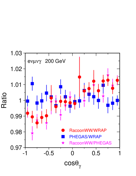
Figure 35: $\cos\theta_{\gamma}$ distributions and ratios for the processes $\nu_{\mu}\mu^{+}e^{-}\overline{\nu}_{e}\gamma$.

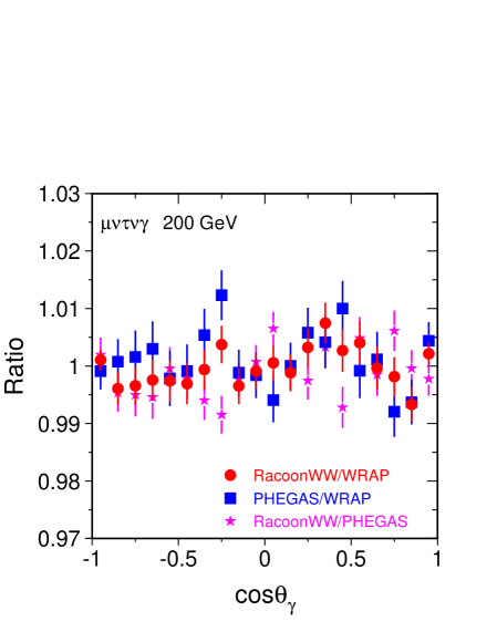
Figure 36: $\cos\theta_{\gamma}$ distributions and ratios for the processes $\nu_{\mu}\mu^{+}\tau^{-}\overline{\nu}_{\tau}\gamma$.

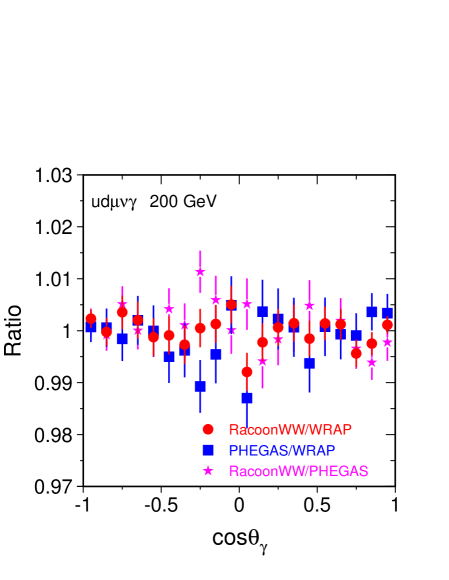
Figure 37: $\cos\theta_{\gamma}$ distributions and ratios for the process $u\overline{d}\mu^{-}\overline{\nu}_{\mu}\gamma$.

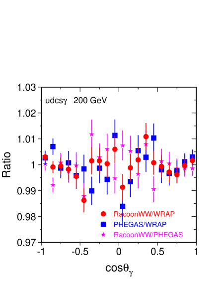
Figure 38: $\cos\theta_{\gamma}$ distribution for the processes $u\overline{d}s\overline{c}\gamma$ and $u\overline{d}e^{-}\overline{\nu}_{e}\gamma$.

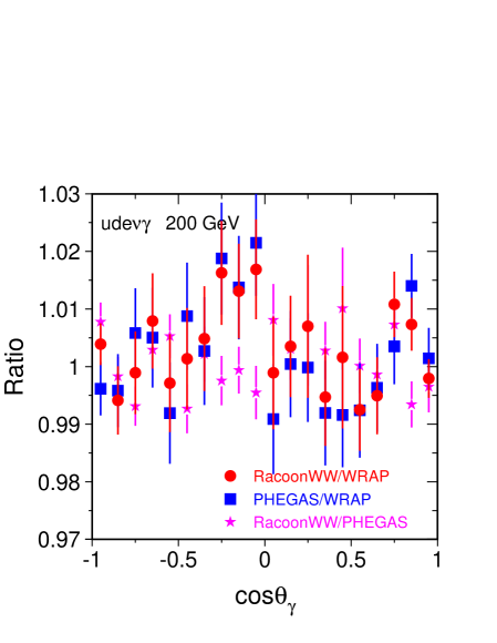
Figure 39: $\cos\theta_{\gamma}$ ratios for the processes $u\overline{d}s\overline{c}\gamma$ and $u\overline{d}e^{-}\overline{\nu}_{e}\gamma$.

Similarly, the $E_{\gamma}$ distributions and ratios in the range [1, 50] GeV are shown for various processes in Figures 40 to 43. Note that virtual corrections are not included, therefore, the photon spectrum starts at some lower boundary of $1\,$GeV. Deviations are of the order of $1\%$ for soft photons and tend to deteriorate for harder ones. Statistically the deviations are compatible with zero. Note that for very hard photons the cross section and therefore the accuracy of the numerical integration of the programs becomes poorer.

In Fig. 44 we show the fermion-photon opening angle $\theta(\gamma,{\rm f})$ (where f is a charged fermion) distribution. In the same figure we show the percentage deviation between the three predictions. The most interesting region occurs for small angles, i.e. towards the collinear region, where a reasonable agreement is registered, of the order of a percent. For the used statistics the deviations are not yet significant. The agreement deteriorates for a larger separation between the photon and the charged particles. However, in this region the cross-section is an order of magnitude lower. Note that the peculiar behavior of the distribution towards $0^{\circ}$ is only due to the fact that the third bin is between $3.6^{\circ}$ and $5.4^{\circ}$ with a cut at $5^{\circ}$.

Finally, we compare the distributions in the bare invariant masses. First the $W^{-}$ one as predicted by WRAP and RacoonWW. Results for all considered channels and for the $W^{-}$-distribution are shown in Fig. 45(left). Note that the curves for the two purely leptonic channels and the two semi-leptonic final states are almost identical. In Fig. 45 (right) we also present the percentage deviations for the process $u\overline{d}s\overline{c}\gamma$. In Fig. 46 we give the corresponding $W^{+}$ invariant-mass distribution including results from the $3$ programs. In Fig. 47 we show the ratio between the $W^{+}$ and the $W^{-}$ invariant-mass distributions from WRAP and RacoonWW respectively.

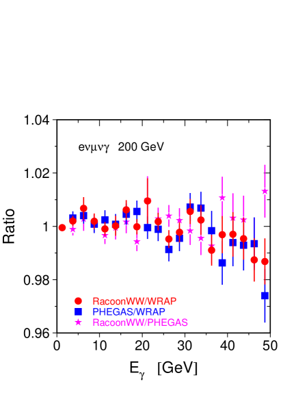
Figure 40: $E_{\gamma}$ distributions and ratios for the process $\nu_{\mu}\mu^{+}e^{-}\overline{\nu}_{e}\gamma$.

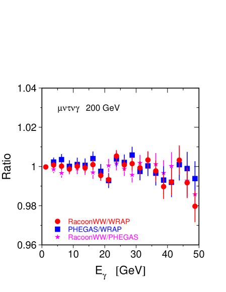
Figure 41: $E_{\gamma}$ distributions and ratios for the process $\nu_{\mu}\mu^{+}\tau^{-}\overline{\nu}_{\tau}\gamma$.

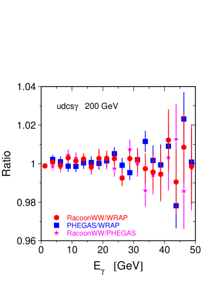
Figure 42: $E_{\gamma}$ distributions and ratios for the process $u\overline{d}s\overline{c}\gamma$.

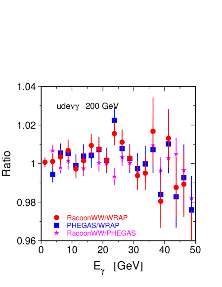
Figure 43: $E_{\gamma}$ distributions and ratios for the process $u\overline{d}e^{-}\overline{\nu}_{e}\gamma$.

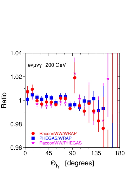
Figure 44: Distribution in the opening angle $\theta(\gamma,{\rm charged~{}fermion})$ between the photon and the nearest charged final-state fermion in the process $e\nu_{e}\mu^{-}\overline{\nu}_{\mu}\gamma$ and the corresponding ratios.

Figure 45: Bare $W^{-}$ mass distributions and percentage deviations between WRAP and RacoonWW for one specific example, $u\overline{d}s\overline{c}\gamma$.

Figure 46: Bare $W^{+}$ mass distributions from WRAP, RacoonWW and PHEGAS.

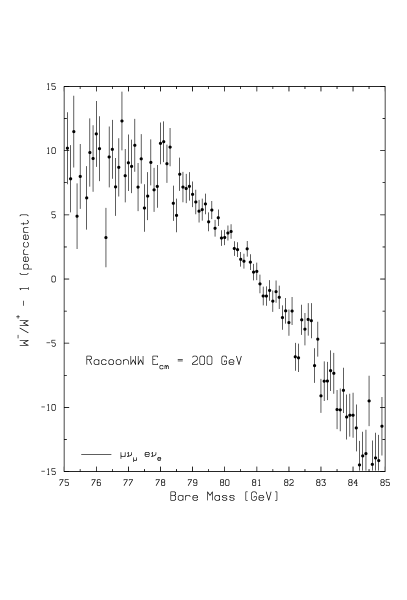
Figure 47: Ratio of invariant mass distributions $W^{-}/W^{+}$ from WRAP and RacoonWW for the process $\mu\nu_{\mu}e\nu_{e}$.

5.3 Estimate of theoretical uncertainty

No global statement can be given, at the moment, on this issue. The following programs have agreed to make individual statements:

RacoonWW

Since the program has only tree-level precision for $e^{+}e^{-}\rightarrow 4{\rm f}+\gamma$, a reliable estimate for the theoretical uncertainty cannot be given with the present version. This could be done if leading corrections such as ISR were included, which is planned in future extensions of the program.

WRAP

WRAP has tried to estimate the theoretical uncertainty in $4{\rm f}+\gamma$ processes coming from variations in the renormalization scheme. The selected process is $e^{+}e^{-}\rightarrow u{\overline{d}}\mu^{-}\bar{\nu}_{\mu}\gamma$ with the cuts used in the tuned comparisons. The following two schemes have been adopted:

$$I)\quad s_{{}_{{\scriptscriptstyle{W}}}}^{2} = 1-\frac{M^{2}_{{}_{W}}}{M^{2}_{{}_{Z}}},\quad\alpha=\frac{4\,\sqrt{2}\,G_{{\scriptscriptstyle{F}}}M^{2}_{{}_{W}}s_{{}_{{\scriptscriptstyle{W}}}}^{2}}{4\,\pi},\quad g^{2}=4\,\pi\,\frac{\alpha}{s_{{}_{{\scriptscriptstyle{W}}}}^{2}},$$

$$II)\quad s_{{}_{{\scriptscriptstyle{W}}}}^{2} = \frac{\pi\alpha(2M_{{}_{W}})}{\sqrt{2}G_{{\scriptscriptstyle{F}}}M^{2}_{{}_{W}}},\quad g^{2}=4\sqrt{2}G_{{\scriptscriptstyle{F}}}M^{2}_{{}_{W}},\quad\mbox{with}\,\,\alpha(2M_{{}_{W}})=128.07.$$ (63)

The cross section is always rescaled by the factor $\alpha(0)/\alpha$ in order to take into account of the scale $\alpha(0)$ for the emitted real photon. Here, $\alpha$ is the value computed in the corresponding renormalization scheme. The results are shown in Tab.(14).

$\sqrt{s}\,$[GeV]	cross section [fb]	$\delta$
200 (I)	75.750(29) fb
200 (II)	75.887(29) fb	$0.18\%$
189 (I)	71.889(25) fb
189 (II)	71.997(25) fb	$0.15\%$
183 (I)	67.238(22) fb
183 (II)	67.324(22) fb	$0.13\%$

Table 14: Estimate of the contribution to the theoretical uncertainty as due to variation of the input parameter set, according to WRAP. I and II refer to the choices in Eq.(63) and $\delta$ is the percentage difference.

Note that the overall theoretical uncertainty for $4{\rm f}+\gamma$ production cannot be below the level of $1\div 2\%$. In this respect the numbers given in Tab.(14) are only a partial indication of possible sources of uncertainty. As shown by the previous analysis, ISR needs to be taken into account in programs for a realistic analysis of $4{\rm f}+\gamma$ final states. Furthermore, in order to avoid double-counting between pre-emission and matrix-element radiation, the implementation of QED corrections in computational tools for $4{\rm f}+\gamma$ processes should rely upon methods, such parton shower, YFS or $p_{t}$-dependent structure functions, able to keep under control photon $p_{t}$ effects. Effects due to finite fermion masses can become important at some percent level for small photon-charged fermion separation cuts.

In order to better understand the uncertainty associated to the implementation of collinear ISR in $4{\rm f}+\gamma$ processes, a comparison between the effects of ISR via collinear SF and $p_{t}$-dependent SF, respectively, is shown in Fig. 26 for the cross section of the the CC10 final state $\mu^{-}\;\overline{\nu}_{\mu}\;u\;\overline{d}\;\gamma$, as a function of the minimum energy of the observed photon, at $\sqrt{s}=192$ GeV. As can be seen, the two prescriptions for ISR can differ at $5\%$ level for $E_{\gamma}^{\rm min}$ close to $1-2\,\,\mathrm{GeV}$, while the difference becomes smaller and smaller as $E_{\gamma}^{\rm min}$ increases. In general, the difference between collinear and $p_{t}$-dependent SF is stronger near the soft and collinear regions, as a priori expected, and it gives an estimate of the size of the double-counting effect at the level of ISR.

NEXTCALIBUR

To check the sensitivity of various distributions to the chosen form of the Structure Functions, the processes $e^{+}e^{-}\rightarrow\mu^{-}\mu^{+}u\overline{u}(\gamma)$ and $e^{+}e^{-}\rightarrow e^{-}\overline{\nu}_{e}u\overline{d}(\gamma)$ have been considered with a slightly different implementation of the sub-leading terms, without observing any significant deviation, at the per mille level, with respect to the previous results.

5.4 Summary and conclusions

While the technical precision in $e^{+}e^{-}\rightarrow 4{\rm f}+\gamma$ does not represent a problem anymore for all those programs that implement an (exact) matrix element, very little effort has been devoted in analyzing the overall theoretical uncertainty. Some of the programs also include the large effect of initial state radiation at the leading logarithmic level. When this is done, the bulk of large radiative corrections is included. Since however in general non-logarithmic ${\mathcal{O}}\left(\alpha\right)$ corrections are not known, the theoretical accuracy is at the level of $2.5\%$ on integrated cross-sections and on inclusive distributions.

6 Single-$W$

Another interesting process at LEP 2 is the so-called single-$W$ production, $e^{+}e^{-}\rightarrow We\nu$ which can be seen as a part of the CC20 process, $e^{+}e^{-}\rightarrow\overline{q}\,q\,(\mu\,\nu_{\mu},\,\,\tau\,\nu_{\tau})\,e\,\nu_{e}$, or as a part of the Mix56 process, $e^{+}e^{-}\rightarrow e^{+}\,e^{-}\,\nu_{e}\,\overline{\nu}_{e}$. For a more detailed theoretical review we refer to [91] and to [92]. All processes in the CC20/Mix56 families are usually considered in two regimes, $|\cos\theta(e^{-})|\geq c$ or SA and $|\cos\theta(e^{-})|\leq c$ or LA. In the list of observables, the single $W$ production is defined by those events that satisfy $|\cos\theta(e^{-})|\geq 0.997$ and therefore is a SA.

The LA cross-section has been computed by many authors and references can be found in [5]. It represents a contribution to the $e^{+}e^{-}\rightarrow W^{+}W^{-}$ total cross-section. From a theoretical point of view the evaluation of a LA cross-section is free of ambiguity, even in the approximation of massless fermions, as long as a gauge-preserving scheme is applied and $\theta(e^{-})$ is not too small.

For SA instead, one cannot employ the massless approximation anymore. In other words, in addition to double-resonant $W$-pair production with one $W$ decaying into $e\nu_{e}$, there are $t$-channel diagrams that give a sizeable contribution for small values of the polar scattering angle of the $t$-channel electron. Single-$W$ processes are sensitive to the breaking of $U(1)$ gauge invariance in the collinear limit, as described in Ref. [7] (see also [93]). The correct way of handling them is based on the so-called Fermion-Loop (FL)scheme [12], the gauge-invariant treatment of the finite-width effects of $W$ and $Z$ bosons in LEP 2 processes. However, till very recently, the Fermion-Loop scheme was available only for the LA-regime. For $e^{+}e^{-}\rightarrow e^{-}\overline{\nu}_{e}f_{1}\overline{f}_{2}$, the $U(1)$ gauge invariance becomes essential in the region of phase space where the angle between the incoming and outgoing electrons is small, see the work of [7] and also an alternative formulations in [11]. In this limit the superficial $1/Q^{4}$ divergence of the propagator structure is reduced to $1/Q^{2}$ by $U(1)$ gauge invariance. In the presence of light fermion masses this gives raise to the familiar $\ln(m^{2}_{e}/s)$ large logarithms. Furthermore, keeping a finite electron mass through the calculation is not enough. One of the main results of [91] was to show that there are remaining subtleties in CC20, associated with the zero mass limit for the remaining fermions.

In [39] a generalization of the Fermion-Loop scheme (hereafter EFL) is introduced to account for external, non-conserved, currents. Another extension has been given in [112] for the imaginary parts of Fermion-Loop contributions, which represents the minimal set for preserving gauge invariance.

The most recent numerical results produced for single-$W$ production are from the following codes [95]: CompHEP, GRC4F, NEXTCALIBUR, SWAP, WPHACT and WTO.

In view of a requested, inclusive cross-section, accuracy of $2\%$ we must include radiative corrections to the best of our knowledge, at least the bulk of any large effect. As we know, the correct scale of the couplings and their differentiation between $s$- and $t$-channel is connected to the real part of the corrections, so that the imaginary FL is not enough, we need a complete FL for single-$W$, or EFL. Having all the parts, the tree-level couplings are replaced by running couplings at the appropriate momenta and the massive gauge-boson propagators are modified accordingly. The vertex coefficients, entering through the Yang–Mills vertex, contain the lowest order couplings as well as the one-loop fermionic vertex corrections.

Each calculation aimed to provide some estimate for single-$W$ production is, at least nominally, a tree level calculation. Among other things it will require the choice of some Input Parameter Set (IPS) and of certain relations among the parameters. Thus, different choices of the basic relations among the input parameters can lead to different results with deviations which, in some case, can be sizeable and should be included in the theoretical uncertainty. Here, more work is needed.

For instance, a possible choice is to fix the coupling constant $g$ as

$$g^{2}={{4\pi\alpha}\over{s_{{}_{{\scriptscriptstyle{W}}}}^{2}}},\quad s_{{}_{{\scriptscriptstyle{W}}}}^{2}={{\pi\alpha}\over{{\sqrt{2}}G_{{\scriptscriptstyle{F}}}M_{{}_{W}}^{2}}},$$ (64)

where $G_{{\scriptscriptstyle{F}}}$ is the Fermi coupling constant. Another possibility would be to use

$$g^{2}=4{\sqrt{2}}G_{{\scriptscriptstyle{F}}}M_{{}_{W}}^{2},$$ (65)

but, in both cases, we miss the correct running of the coupling. Ad hoc solutions should be avoided, and the running of the parameters must always follow from a fully consistent scheme.

Another important issue in dealing with single-$W$ production is connected with the inclusion of QED radiation. It is well known that universal, $s$-channel structure functions are not adequate enough to include the radiation since they generate an excess of ISR bremsstrahlung. In $t$-channel dominated processes the interference between incoming fermions becomes very small while the destructive interference between initial and final states becomes strong.

It is quite a known fact that, among the electroweak corrections, QED radiation gives the largest contribution and the needed precision requires a re-summation of the large logarithms. For annihilation processes, $e^{+}e^{-}\rightarrow\overline{f}f$, initial state radiation is a definable, gauge-invariant concept and we have general tools to deal with it; the structure function approach and also the parton-shower method. However, when we try to apply the algorithm to four-fermion processes that include non-annihilation channels we face a problem: it is still possible to include the large universal logarithms by making use of the standard tools but an appropriate choice of scale is mandatory. Such is the case in single-$W$. The problem of the correct scale to be used in QED corrections has been tackled by two groups, GRACE and SWAP and additional results will be shown in Sub-Sects. 6.2.1, 6.2 and in Sub-Sect. 6.2.

6.1 Signal definition in single-$W$

The experimental requirements on single-$W$ are:

• CC20 – Mix56 calculations with some detector acceptance that are used for a) triple gauge coupling determination, b) standard model background to searches;

• the LEP EWWG cross-section definition that is used to combine the cross-section measurements from the four LEP experiments.

During the last WW99 Crete Workshop a proposal has been made to reach a common signal definition for the LEP EWWG cross-section [96]. The persons who participated in the WW99 workshop agreed on some setup to define the single-$W$ production and now this has been formalized in one of the LEP EWWG meetings; there, it was decided to have a combination of the single-$W$ cross-section using the signal definitions of Tab.(15) for $e^{+}e^{-}\rightarrow e^{-}\overline{\nu}_{e}f^{\prime}\overline{f}$: The set of $t$-channel diagrams, all for CC20, are shown in Fig. 48. The signal definition uses $10$ diagrams for CC20, $9$ for CC18 and $37$ for Mix56.

Process	diagrams	cuts
$ee\nu\nu$	$t$-channel only	$E(e^{+})>20\,\,\mathrm{GeV},|\cos\theta(e^{+})|<0.95,|\cos\theta(e-)|>0.95$
$e\nu\mu\nu$	$t$-channel only	$E_{(}\mu^{+})>20\,\,\mathrm{GeV}$
$e\nu\tau\nu$	$t$-channel only	$E_{(}\tau^{+})>20\,\,\mathrm{GeV}$
$e\nu ud$	$t$-channel only	$M(ud)>45GeV$
$e\nu cs$	$t$-channel only	$M(cs)>45GeV$

Table 15: Signal definition for single-$W$ processes.

Note that charge-conjugate state should be taken into account and that an asymmetric cut has been introduced for $ee\nu\nu$; the latter is due to the fact that the process itself is CP-even when no cut is applied, but an ambiguity remains if one starts to discuss single-$W$ with $e^{-}$ in the forward direction. Then we should multiply this process by a factor $2$ as well. The goal of this common definition is to be able to combine the different $e\nu\overline{q}q,e\nu\mu\nu,e\nu\tau\nu,e\nu e\nu$ measurements from different experiments so that the new theoretical calculations can be checked with data at a level better than $10\%$.

Signal definition has a longstanding tradition in LEP physics, the most celebrated being the $t$-channel subtraction in Bhabha and the most recent being the CC03 cross-section. Here we have a different situation. First of all, nobody has radiative corrections for single-$W$ production, hence the usual argument of the availability of a sophisticated semi-analytical calculation for the signal does not apply. We could avoid a definition of the signal in terms of diagrams and have recourse to a definition in terms of cuts since, in a very narrow cone around the beam axis, the single-$W$ family is fully dominated by the $t$-channel photons.

$$\begin{array}[]{ccc}\vbox{\hbox{ \begin{picture}(110.0,100.0)(0.0,0.0) \put(0.0,0.0){} \put(0.0,0.0){} \put(0.0,0.0){} \put(0.0,0.0){} \put(0.0,0.0){} \put(0.0,0.0){} \put(0.0,0.0){} \put(0.0,0.0){} \put(0.0,0.0){} \raise 98.0pt\hbox to0.0pt{\kern-14.0pt\makebox(0.0,0.0)[lc]{$e^{+}$}\hss} \ignorespaces \raise 98.0pt\hbox to0.0pt{\kern 77.0pt\makebox(0.0,0.0)[lc]{$\overline{\nu}_{e}$}\hss} \ignorespaces \raise 0.0pt\hbox to0.0pt{\kern-14.0pt\makebox(0.0,0.0)[lc]{$e^{-}$}\hss} \ignorespaces \raise 0.0pt\hbox to0.0pt{\kern 77.0pt\makebox(0.0,0.0)[lc]{$e^{-}$}\hss} \ignorespaces \raise 77.0pt\hbox to0.0pt{\kern 77.0pt\makebox(0.0,0.0)[lc]{$\overline{d}$}\hss} \ignorespaces \raise 21.0pt\hbox to0.0pt{\kern 77.0pt\makebox(0.0,0.0)[lc]{$u$}\hss} \ignorespaces \raise 60.0pt\hbox to0.0pt{\kern 18.0pt\makebox(0.0,0.0)[lc]{$W$}\hss} \ignorespaces \raise 26.0pt\hbox to0.0pt{\kern 11.0pt\makebox(0.0,0.0)[lc]{$\gamma,Z$}\hss} \ignorespaces \end{picture}}}&\quad+&\vbox{\hbox{ \begin{picture}(110.0,100.0)(0.0,0.0) \put(0.0,0.0){} \put(0.0,0.0){} \put(0.0,0.0){} \put(0.0,0.0){} \put(0.0,0.0){} \put(0.0,0.0){} \put(0.0,0.0){} \put(0.0,0.0){} \put(0.0,0.0){} \raise 77.0pt\hbox to0.0pt{\kern 77.0pt\makebox(0.0,0.0)[lc]{$\overline{d}$}\hss} \ignorespaces \raise 21.0pt\hbox to0.0pt{\kern 77.0pt\makebox(0.0,0.0)[lc]{$u$}\hss} \ignorespaces \raise 76.0pt\hbox to0.0pt{\kern 54.0pt\makebox(0.0,0.0)[lc]{$W$}\hss} \ignorespaces \raise 66.0pt\hbox to0.0pt{\kern 11.0pt\makebox(0.0,0.0)[lc]{$\gamma,Z$}\hss} \ignorespaces \raise 98.0pt\hbox to0.0pt{\kern-14.0pt\makebox(0.0,0.0)[lc]{$e^{+}$}\hss} \ignorespaces \raise 98.0pt\hbox to0.0pt{\kern 77.0pt\makebox(0.0,0.0)[lc]{$\overline{\nu}_{e}$}\hss} \ignorespaces \raise 0.0pt\hbox to0.0pt{\kern-14.0pt\makebox(0.0,0.0)[lc]{$e^{-}$}\hss} \ignorespaces \raise 0.0pt\hbox to0.0pt{\kern 77.0pt\makebox(0.0,0.0)[lc]{$e^{-}$}\hss} \ignorespaces \end{picture}}}\end{array}$$

$$\begin{array}[]{ccc}\vbox{\hbox{ \begin{picture}(110.0,100.0)(0.0,0.0) \put(0.0,0.0){} \put(0.0,0.0){} \put(0.0,0.0){} \put(0.0,0.0){} \put(0.0,0.0){} \put(0.0,0.0){} \put(0.0,0.0){} \put(0.0,0.0){} \put(0.0,0.0){} \raise 72.0pt\hbox to0.0pt{\kern 77.0pt\makebox(0.0,0.0)[lc]{$\overline{d}$}\hss} \ignorespaces \raise 26.0pt\hbox to0.0pt{\kern 77.0pt\makebox(0.0,0.0)[lc]{$u$}\hss} \ignorespaces \raise 52.0pt\hbox to0.0pt{\kern 22.0pt\makebox(0.0,0.0)[lc]{$u$}\hss} \ignorespaces \raise 20.0pt\hbox to0.0pt{\kern 10.0pt\makebox(0.0,0.0)[lc]{$\gamma,Z$}\hss} \ignorespaces \raise 77.0pt\hbox to0.0pt{\kern 17.0pt\makebox(0.0,0.0)[lc]{$W$}\hss} \ignorespaces \raise 98.0pt\hbox to0.0pt{\kern-14.0pt\makebox(0.0,0.0)[lc]{$e^{+}$}\hss} \ignorespaces \raise 98.0pt\hbox to0.0pt{\kern 77.0pt\makebox(0.0,0.0)[lc]{$\overline{\nu}_{e}$}\hss} \ignorespaces \raise 0.0pt\hbox to0.0pt{\kern-14.0pt\makebox(0.0,0.0)[lc]{$e^{-}$}\hss} \ignorespaces \raise 0.0pt\hbox to0.0pt{\kern 77.0pt\makebox(0.0,0.0)[lc]{$e^{-}$}\hss} \ignorespaces \end{picture}}}&\quad+&\vbox{\hbox{ \begin{picture}(110.0,100.0)(0.0,0.0) \put(0.0,0.0){} \put(0.0,0.0){} \put(0.0,0.0){} \put(0.0,0.0){} \put(0.0,0.0){} \put(0.0,0.0){} \put(0.0,0.0){} \put(0.0,0.0){} \put(0.0,0.0){} \put(0.0,0.0){} \raise 72.0pt\hbox to0.0pt{\kern 77.0pt\makebox(0.0,0.0)[lc]{$\overline{d}$}\hss} \ignorespaces \raise 21.0pt\hbox to0.0pt{\kern 77.0pt\makebox(0.0,0.0)[lc]{$u$}\hss} \ignorespaces \raise 52.0pt\hbox to0.0pt{\kern 22.0pt\makebox(0.0,0.0)[lc]{$d$}\hss} \ignorespaces \raise 20.0pt\hbox to0.0pt{\kern 10.0pt\makebox(0.0,0.0)[lc]{$\gamma,Z$}\hss} \ignorespaces \raise 77.0pt\hbox to0.0pt{\kern 17.0pt\makebox(0.0,0.0)[lc]{$W$}\hss} \ignorespaces \raise 98.0pt\hbox to0.0pt{\kern-14.0pt\makebox(0.0,0.0)[lc]{$e^{+}$}\hss} \ignorespaces \raise 98.0pt\hbox to0.0pt{\kern 77.0pt\makebox(0.0,0.0)[lc]{$\overline{\nu}_{e}$}\hss} \ignorespaces \raise 0.0pt\hbox to0.0pt{\kern-14.0pt\makebox(0.0,0.0)[lc]{$e^{-}$}\hss} \ignorespaces \raise 0.0pt\hbox to0.0pt{\kern 77.0pt\makebox(0.0,0.0)[lc]{$e^{-}$}\hss} \ignorespaces \end{picture}}}\end{array}$$

$$\begin{array}[]{ccc}\vbox{\hbox{ \begin{picture}(110.0,100.0)(0.0,0.0) \put(0.0,0.0){} \put(0.0,0.0){} \put(0.0,0.0){} \put(0.0,0.0){} \put(0.0,0.0){} \put(0.0,0.0){} \put(0.0,0.0){} \put(0.0,0.0){} \raise 77.0pt\hbox to0.0pt{\kern 77.0pt\makebox(0.0,0.0)[lc]{$\overline{d}$}\hss} \ignorespaces \raise 21.0pt\hbox to0.0pt{\kern 77.0pt\makebox(0.0,0.0)[lc]{$u$}\hss} \ignorespaces \raise 71.0pt\hbox to0.0pt{\kern 48.0pt\makebox(0.0,0.0)[lc]{$W$}\hss} \ignorespaces \raise 56.0pt\hbox to0.0pt{\kern 21.0pt\makebox(0.0,0.0)[lc]{$Z$}\hss} \ignorespaces \raise 98.0pt\hbox to0.0pt{\kern-14.0pt\makebox(0.0,0.0)[lc]{$e^{+}$}\hss} \ignorespaces \raise 98.0pt\hbox to0.0pt{\kern 77.0pt\makebox(0.0,0.0)[lc]{$\overline{\nu}_{e}$}\hss} \ignorespaces \raise 0.0pt\hbox to0.0pt{\kern-14.0pt\makebox(0.0,0.0)[lc]{$e^{-}$}\hss} \ignorespaces \raise 0.0pt\hbox to0.0pt{\kern 77.0pt\makebox(0.0,0.0)[lc]{$e^{-}$}\hss} \ignorespaces \end{picture}}}&\quad+&\vbox{\hbox{ \begin{picture}(110.0,100.0)(0.0,0.0) \put(0.0,0.0){} \put(0.0,0.0){} \put(0.0,0.0){} \put(0.0,0.0){} \put(0.0,0.0){} \put(0.0,0.0){} \put(0.0,0.0){} \put(0.0,0.0){} \raise 77.0pt\hbox to0.0pt{\kern 77.0pt\makebox(0.0,0.0)[lc]{$\overline{d}$}\hss} \ignorespaces \raise 21.0pt\hbox to0.0pt{\kern 77.0pt\makebox(0.0,0.0)[lc]{$u$}\hss} \ignorespaces \raise 41.0pt\hbox to0.0pt{\kern 40.0pt\makebox(0.0,0.0)[lc]{$W$}\hss} \ignorespaces \raise 56.0pt\hbox to0.0pt{\kern 19.0pt\makebox(0.0,0.0)[lc]{$W$}\hss} \ignorespaces \raise 98.0pt\hbox to0.0pt{\kern-14.0pt\makebox(0.0,0.0)[lc]{$e^{+}$}\hss} \ignorespaces \raise 98.0pt\hbox to0.0pt{\kern 77.0pt\makebox(0.0,0.0)[lc]{$\overline{\nu}_{e}$}\hss} \ignorespaces \raise 0.0pt\hbox to0.0pt{\kern-14.0pt\makebox(0.0,0.0)[lc]{$e^{-}$}\hss} \ignorespaces \raise 0.0pt\hbox to0.0pt{\kern 77.0pt\makebox(0.0,0.0)[lc]{$e^{-}$}\hss} \ignorespaces \end{picture}}}\end{array}$$

Figure 48: The $t$-channel component of the CC20 family of diagrams: fusion, bremsstrahlung and multi-peripheral.

6.1.1 A study of single-$W$ signal definition with CompHEP

Authors

E. Boos, M. Dubinin and V. Ilyin

Single-$W$ signal definition in the reaction $e^{+}e^{-}\rightarrow e^{+}e^{-}\nu_{e}\overline{\nu}_{e}$

It is well-known for a long time how the single $W$ signal can be separated with the help of kinematical cuts [93]. The typical set of cuts used by ALEPH, DELPHI and L3 collaborations for the leptonic four fermion states $e^{-}\overline{\nu}_{e}l^{+}\nu_{l}$ separates the configurations with very forward $e^{-}$ and a rather energetic $l^{+}$ produced at a sufficiently large angle with the beam. For instance, the L3 cuts to be used in the following calculations are $|\cos\theta_{e^{-}}|\geq 0.997$, $E_{l}\geq 15\,\,\mathrm{GeV}$ and $|\cos\theta_{l^{+}}|\leq 0.997$. In the case of the semi-leptonic states $e^{-}\overline{\nu}_{e}q\overline{q}^{{}^{\prime}}$ an additional cut $M(q\overline{q}^{{}^{\prime}})\geq$ 45 GeV have been applied by OPAL. In so far as different collaborations are using not exactly the same cuts (defined by the optimal detector acceptance), the definition of the $W$ signal in terms of angular cuts is not universal and some standardization procedure is needed. In the recent proposal by LEP experiments [96] the OPAL collaboration considered the possibility to introduce the definition of the $W$ signal in terms of diagrams. Angular cuts on the forward electron and the corresponding anti-lepton are not imposed, so the single $W$ cross-section depends only on the $E_{l}$ energy cut and is defined by the gauge invariant subset of the $t$-channel single resonant diagrams. The universality of such definition is satisfactory if the interferences between the gauge invariant subsets of diagrams in the channels $e^{-}\overline{\nu}_{e}l^{+}\nu_{l}$ and $e^{-}\overline{\nu}_{e}q\overline{q}^{{}^{\prime}}$ are always negligible. Then indeed the single $W$ cross-section in terms of diagrams could be meaningful.

We performed a detailed calculation of the contributions from various diagram sets of the Mix56 channel $e^{+}e^{-}\rightarrow e^{+}e^{-}\nu_{e}\overline{\nu}_{e}$ (see Appendix for Fig. 63-Fig. 70 referred to in the following). Using the general approach to the amplitude decomposition into gauge invariant classes [131], we found ten gauge invariant subsets of diagrams (see Fig. 63-Fig. 64). In Tab.(16) $18W$ denotes two gauge invariant subsets of $9$ diagrams with single $W$ (see Fig. 63), $8Z$ denotes two gauge invariant subsets of $4$ diagrams with single $Z$ (see Fig. 64), $9W^{+}W^{-}$ stands for the double-resonant subset (Fig. 65) and so on. Main contribution to the final configurations with forward electron come from the single $W$ and the single $Z$ production, while various $\gamma,Z\rightarrow e^{+}e^{-}$ conversion corrections (Fig. 68-Fig. 70) to the $e^{+}e^{-}\rightarrow e^{+}e^{-},\,\nu_{e}\overline{\nu}_{e}$ are negligible. For the case of angular cuts on the forward electron the interference between the single $W$ and single $Z$ subsets $18W$ and $8Z$ is negative and equal to several fb. However, if the angular cuts are removed, the destructive interference modulo increases rather considerably (Table 16). This is not an unexpected fact since both single-$W$ and single-$Z$ (NC processes with one lost electron) subsets have a similar $t$-channel pole structure. Other interferences are also not negligible. So in the case of $e^{+}e^{-}\nu_{e}\overline{\nu}_{e}$ channel the diagram-based definition of single $W$ signal is not completely satisfactory.

	26 $t$-ch.	18$W$	8$Z$	9$W^{+}W^{-}$	4$ZZ$	9$\nu_{e}\overline{\nu}_{e}$	4$e^{+}e^{-}$	2$\nu_{e}\overline{\nu}_{e}$	2 $t$-ch
$\theta_{e}$,$E_{l}$	49.9	36.1	16.4	0.91	0.02	8$\cdot$10-3	7$\cdot$10-5	1$\cdot$10-5	6$\cdot$10-7
only $E_{l}$	220.5	106.6	153.6	240.5	44.9	15.9	0.02	3$\cdot$10-3	8$\cdot$10-4

Table 16: Contributions of the gauge invariant subsets (fb) at the energy $\sqrt{s}=$200 GeV. First row - with angular cuts, second row - no angular cuts for $e^{-}$, $e^{+}$. The result for 26 $t$-channel diagrams (18$W$ and 8$Z$, see Fig.1,2) is indicated in the second column.

6.2 Description of the programs, results and comparisons

WTO and EFL

Author

G. Passarino

The Fermion-Loop scheme (EFL)

The EFL scheme for non-conserved currents is described in Ref. [39] and briefly discussed in Sect. 3.8.1. It consists of the re-summation of the fermionic one-loop corrections to the vector-vector, vector-scalar and scalar-scalar propagators and of the inclusion of all remaining fermionic one-loop corrections, in particular those to the Yang–Mills vertices.

In the original formulation, the Fermion-Loop scheme requires that vector bosons couple to conserved currents, i.e. , that the masses of all external fermions can be neglected. There are several examples where fermion masses must be kept to obtain a reliable prediction. As already stated, this is the case for the single-$W$ production mechanism, where the outgoing electron is collinear, within a small cone, with the incoming electron. Therefore, $m_{e}$ cannot be neglected. Furthermore, among the $20$ Feynman diagrams that contribute (for $e\overline{\nu}_{e}u\overline{d}$ final states, up to $56$ for $e^{+}e^{-}\nu_{e}\overline{\nu}_{e}$) there are multi-peripheral ones that require a non-vanishing mass also for the other outgoing fermions.

As well known in the literature, the Fixed-Width scheme behaves properly in the collinear and high-energy regions of phase space, to the contrary of the Running-Width scheme, but it completely misses the running of the couplings, an effect that is expected to be above the requested precision tag of $2\%$. To be specific the name of Fixed-Width scheme is reserved for the following: the cross-section is computed using the tree-level amplitude. The massive gauge-boson propagators are given by $1/(p^{2}-m^{2}+i\Gamma m)$. This gives an unphysical width in $t$-channel, but retains $U(1)$ gauge invariance in the CC20 process.

The correct way of handling this problem is to apply the EFL-scheme and, by considering the impact of the EFL-scheme on the relevant observables, one is able to judge on the goodness of naive rescaling procedures or of any incomplete FL-scheme. One of the problem with the latter is that vertices, although chosen to respect gauge-invariance, are not uniquely defined. Furthermore, couplings other than $\alpha_{\rm QED}$ usually do not evolve with the scale and complex poles, the truly gauge-invariant quantities, are never introduced or explicitly computed. Finally, programs than cannot split diagrams and apply an overall rescaling, both in $s$- and $t$-channel, mistreat single-$W$ and/or violates $SU(2)$ invariance.

Numerical results and recommendations.

Numerical results for EFL have been shown in Ref. [115]. Here, we limit the presentation to some useful recommendations:

• the bulk of the effect is in the running of the e.m. coupling constant;

• one can compute the single-$W$ cross-sections for a fixed mass of the top quark, such as $m_{t}=173.8\,$GeV, without finding any significative difference with the case where $m_{t}$ is fixed by a consistency relation. We are using complex-mass renormalization but we only include fermionic corrections. Therefore, we can start with the Fermi coupling constant but also with $M_{{}_{W}}$ as an input parameter. Equating the corresponding renormalization conditions yields a relation between $M_{{}_{Z}}$, $G_{{\scriptscriptstyle{F}}}$, ${\rm{Re}}\{\alpha(M^{2}_{{}_{Z}})^{-1}\}$, $M_{{}_{W}}$, and $m_{t}$, see [12]. This relation can be solved iteratively for $m_{t}$. For the following input parameter set, $M_{{}_{W}}=80.350\,\,\mathrm{GeV}$, $M_{{}_{Z}}=91.1867\,\,\mathrm{GeV}$ and $G_{{\scriptscriptstyle{F}}}=1.16639\,\times\,10^{-5}\,\,\mathrm{GeV}^{-2}$, we obtain the following solution:

  $$\mu_{{\scriptscriptstyle{W}}}=\sqrt{{\rm{Re}}\left(p_{{}_{W}}\right)}=80.324\,\,\mathrm{GeV},\quad\gamma_{{\scriptscriptstyle{W}}}=-{{{\rm{Im}}\left(p_{{}_{W}}\right)}\over{\mu_{{\scriptscriptstyle{W}}}}}=2.0581\,\,\mathrm{GeV},\quad m_{t}=148.62\,\,\mathrm{GeV},$$ (69)

  with $26\,\,\mathrm{MeV}$ difference between $M_{{}_{W}}$ and $\mu_{{\scriptscriptstyle{W}}}$. See Sect. 6.3.1 for the inclusion of QCD effects. This type of effect should be included in any incomplete FL-scheme;

• the main accent in the EFL-scheme is on putting the correct scale in the running of $\alpha_{\rm QED}$. The latter is particularly important for the $t$-channel diagrams, dominated by a scale $q^{2}\approx 0$ and not $q^{2}\approx M^{2}_{{}_{W}}$. However, a consistent implementation of radiative corrections does more than evolving $\alpha_{\rm QED}$ to the correct scale, other couplings are also running, propagators are modified and vertices are included;

• the effective FW-scheme describes considerably well the hadronic final state with a cut of $M(u\overline{d})>45\,$GeV. However, the diminution induced by $\alpha_{\rm QED}(q^{2})$ is too large for the leptonic final state. The latter is a clear sign that other effects are relevant and a naive rescaling does not suffice in reproducing a realistic approximation in all situations, at least not within the $2\%$ level of requested theoretical accuracy;

• Modifications induced by the fermionic loops are sensitive to the relative weight of single-resonant terms and of multi-peripheral peaks. Furthermore, the effect of radiative corrections inside the $W$-propagators ($\rho$-factors of Ref. [115]) is far from being negligible and tends to compensate the change due to the running of $\alpha_{\rm QED}$.

These recommendations are better illustrated by few examples. At $\sqrt{s}=183\,$GeV we consider the angular distribution, $d\sigma/d\theta_{e}$ for the $u\overline{d}e^{-}\overline{\nu}_{e}$ final states. The results are shown in Fig. 49.

Figure 49: WTO predictions for $d\sigma/d\cos\theta_{e}$ [fb/degrees] for $e^{+}e^{-}\rightarrow u\overline{d}e^{-}\overline{\nu}_{e}$ with $M(u\overline{d})>45\,$GeV and $\sqrt{s}=183\,\,\mathrm{GeV}$.

From Fig. 49 we see that the EFL prediction is lower than the FW one, from $-7.46\%$ in the bin $0^{\circ}-0.1^{\circ}$ to $-5.56\%$ in the bin $0.3^{\circ}-0.4^{\circ}$. Correspondingly, the first bin is $6.78$ higher than the second one, $11.60(16.37)$ than the third(fourth) one. This is not a surprise, since the first bin represents $50\%$ of the total single-$W$ cross-section.

Always in the same figure, we have reported the behavior of $\Bigl{[}\alpha(q^{2})/\alpha_{G_{{\scriptscriptstyle{F}}}}-1\Bigr{]}^{2}$ as a function of $\theta_{e}$ for three values of $y$, using the appropriate relation: $q^{2}=q^{2}(\theta_{e},y)$, $y$ being the fraction of the electron energy carried by the photon. The behavior of EFL/FW-1, when we vary $\theta_{e}$, is very similar to the one given by the ratio of coupling constants, indicating that the bulk of the effect is in the running of the e.m. coupling constant.

For completeness we have reported the numerical results for the three energies in Tab.(17), where the first entry is Fixed-Width distribution and the second entry is EFL one. Only the first four bins are shown, owing to the fact that they are the most significant in the distribution. The third entry in Tab.(17) gives EFL/FW-1 in percent.

$\theta_{e}\,$[Deg]	$\sqrt{s}=183\,\,\mathrm{GeV}$	$\sqrt{s}=189\,\,\mathrm{GeV}$	$\sqrt{s}=200\,\,\mathrm{GeV}$
$0.0^{\circ}\div 0.1^{\circ}$	0.48395	0.54721	0.67147
	0.44784	0.50695	0.62357
	-7.46	-7.36	-7.13
$0.1^{\circ}\div 0.2^{\circ}$	0.07026	0.07815	0.09323
	0.06605	0.07357	0.08798
	-5.99	-5.86	-5.63
$0.2^{\circ}\div 0.3^{\circ}$	0.04095	0.04554	0.05433
	0.03860	0.04298	0.05141
	-5.74	-5.62	-5.37
$0.3^{\circ}\div 0.4^{\circ}$	0.02897	0.03223	0.03845
	0.02736	0.03045	0.03646
	-5.56	-5.52	-5.18

Table 17: $d\sigma/d\theta_{e}$ in [pb/degrees], from WTO, for the process $e^{+}e^{-}\rightarrow e^{-}\overline{\nu}_{e}u\overline{d}$, for $M(u\overline{d})>45\,$GeV. First entry is Fixed-Width distribution, second entry is Fermion-Loop one and third entry is EFL/FW-1 in percent.

Next we consider $e^{+}e^{-}\rightarrow e\nu\mu\nu$, with $|\cos\theta_{e}|>0.997$, $E_{\mu}>15\,$GeV, and $|\cos\theta_{\mu}|<0.95$. In Tab.(18) we report the comparison between the EFL distribution and the FW one for $\sqrt{s}=183\,$GeV. As before, only the most significant bins are shown ($0.0^{\circ}\div 0.4^{\circ}$).

$\theta_{e}\,$[Deg]	FW	EFL	EFL/FW-1 (percent)
$0.0^{\circ}\div 0.1^{\circ}$	0.14154	0.13448	-4.99
$0.1^{\circ}\div 0.2^{\circ}$	0.02113	0.02031	-3.88
$0.2^{\circ}\div 0.3^{\circ}$	0.01238	0.01194	-3.55
$0.3^{\circ}\div 0.4^{\circ}$	0.00880	0.00851	-3.30

Table 18: $d\sigma/d\theta_{e}$ in [pb/degrees], from WTO, for the process $e^{+}e^{-}\rightarrow e^{-}\overline{\nu}_{e}\nu_{\mu}\mu^{+}$, for $|\cos\theta_{e}|>0.997$, $E_{\mu}>15\,$GeV, and $|\cos\theta_{\mu}|<0.95$. Furthermore, $\sqrt{s}=183\,$GeV.

As for the hadronic case, the EFL prediction is considerably lower than the FW one, although the percentage difference between the two is approximately $2.2\%\div 2.4\%$ smaller than in the previous case. Useful comparisons will be presented in the WPHACT description of this Section.

A final comment will be devoted to QED ISR. Very often one can find the statement that the choice of the appropriate scale in the structure functions is mandatory. This is a jargon for ‘implementing the correct exponentiation factor in multi-photon emission’. Note that the usual infrared exponent $\alpha\,B$ is represented by

$$\alpha\,B = \frac{2\,\alpha}{\pi}\,\big{[}\frac{1+r^{2}}{1-r^{2}}\,\ln\left(\frac{1}{r}\right)-1\big{]}\sim\frac{2\,\alpha}{\pi}\,\left(\ln\frac{Q^{2}}{m^{2}}-1\right),\quad\mbox{for}\quad Q^{2}\gg m^{2},$$

$$\frac{m^{2}}{Q^{2}} = \frac{r}{(1-r)^{2}}\sim r,$$ (70)

where $Q^{2}$ is the Mandelstam invariant associated with the emitting pair. For $|t|\gg m^{2}_{e}$ the photon radiation is governed by $\ln(|t|/m^{2}_{e})$ rather than by $\ln(s/m^{2}_{e})$. The difference is again a large log and explain the excess of radiation generated by $s$-channel SF. However, the whole expression for $B$ is known and not only its asymptotic behavior (the scale). Therefore, for vanishing scattering angles, the correct behavior should be read from Eq.(70). In this respect one should remember that $|t_{\gamma}|_{\rm min}$ in single-$W$ can be much lower than $m^{2}_{e}$, being $m^{2}_{e}y^{2}/(1-y)$ where $y=M^{2}(\nu_{e}f_{1}\overline{f}_{2})/s$.

Single-$W$ with WPHACT

Authors

E. Accomando, A. Ballestrero and E. Maina

A new version of WPHACT [127] is now available. It includes all massive matrix elements in addition to the previous ones which accounted for $b$-quark masses only. As before, the matrix elements are computed with the method of Ref. [126], which has proved to be fast and reliable in particular for massive calculations. New mappings of the phase space have been added, in order to account in an efficient way for the peaking structure of contributions like single-$W$, single-$Z$ and $\gamma\gamma$ contributions. With the new version one has, therefore, the choice of using fully massive or massless calculations. The former are needed in various processes which diverge for massless fermions , while the latter are faster and give an excellent approximation for most cases. We start with the introduction of the IFL-scheme showing comparisons with alternative solutions, designed to deal with gauge-invariance issues. However, the most important part is contained in the second Subsection where the effective scaling induced by $\alpha_{\rm QED}$ is presented.

IFL-scheme

The Imaginary Part Fermion-Loop scheme has been generalized to the fully massive case of non-conserved weak currents in Ref. [112]. The results obtained have been compared with other gauge restoring schemes used in single-$W$ processes computations. The following schemes have been considered in the analysis:

• Imaginary-part FL scheme(IFL): The imaginary part of the fermion-loop corrections, as computed in Ref. [112], are used. Fermion masses are neglected only in loops but not in the rest of the diagrams.

• Fixed width(FW): The $\mathrm{W}$-boson propagators show an unphysical width for $p^{2}<0$, but retains $U(1)$ gauge invariance in the CC20 process [7].

• Complex Mass(CM): All weak boson masses squared $M^{2}_{{}_{B}}\;,B=W,Z$ are changed to $M^{2}_{{\scriptscriptstyle{B}}}-i\,M_{{\scriptscriptstyle{B}}}\Gamma_{{\scriptscriptstyle{B}}}$ [18] ($\Gamma_{{\scriptscriptstyle{B}}}$ is the on-shell $B$ width), including when they appear in the definition of the weak mixing angle. This scheme, which again gives an unphysical width in some cases, has however the advantage of preserving both $U(1)$ and $SU(2)$ Ward identities.

• Overall scheme(OA): The diagrams for $e^{-}e^{+}\rightarrow e^{-}\bar{\nu}_{e}u\bar{d}$ can be split into two sets that are separately gauge invariant under $U(1)$. In the actual implementation of the OA-scheme, $t$ channel diagrams are computed without any width and are then multiplied by $(q^{2}-M^{2})/(q^{2}-M^{2}+iM\Gamma)$ where $q$, $M$ and $\Gamma$ are the momentum, the mass and the width of the possibly-resonant $\mathrm{W}$-boson. This scheme retains $U(1)$ gauge invariance at the expenses of a mistreatment of the non-resonant terms.

In order to asses the relevance of current non-conservation, the imaginary part of the fermion-loop corrections have also been implemented with the assumption that all currents that couple to the fermion-loop are conserved. In this case the expressions of Ref. [112] reduce to those computed in  [7]. Note that the masses of external fermions are nonetheless taken into account in the calculation of the matrix elements. This scheme violates $U(1)$ gauge-invariance by terms which are proportional to the fermion masses squared, as already noted in Ref. [94]. However they are enhanced at high energy by large factors and can be numerically quite relevant. This scheme will be referred to as the imaginary-part FL scheme with conserved currents (hereafter IFLCC). All schemes described above have been implemented in the new version of WPHACT [127] with the fully massive option.

	190 GeV	800 GeV	1500 GeV
IFL	0.11815 (13)	1.6978 (15)	3.0414 (35)
FW	0.11798 (11)	1.6948 (12)	3.0453 (41)
CM	0.11791 (12)	1.6953 (16)	3.0529 (60)
OA	0.11760 (10)	1.6953 (13)	3.0401 (23)
IFLCC	0.11813 (12)	1.7987 (16)	5.0706 (44)

Table 19: Cross-sections in pb for the processes $e^{+}e^{-}~{}\rightarrow\;e^{-}\bar{\nu}_{e}u\overline{d}$ for various gauge restoring schemes. No ISR is included and we apply the following cuts: $M(u\overline{d})>5\,\mathrm{GeV}\;,E_{u}>3\,\mathrm{GeV},E_{\overline{d}}>3\,\mathrm{GeV},\cos(\theta_{e})>.997$

In Tab.(19) the cross-sections for CC20 are given for the different gauge restoring schemes at LEP 2 and LC energies. From it, one can immediately deduce that the IFL, FW, CM and the OA schemes agree within $2\,\sigma$ in almost all cases. The IFLCC scheme agrees with the other ones at LEP 2 energies but already at 800 $\,\mathrm{GeV}$ it overestimates the total cross-section by about $6\%$. At $1.5\;\mathrm{TeV}$ the error is almost a factor of two. On the contrary, even in the presence of non–conserved currents, i.e. of massive external fermions, the FW CM and OA calculations give predictions which are in agreement, within a few per mil, with the IFL scheme. The agreement with the results of a self-consistent approach justifies, from a practical point of view, the ongoing use of the FW, CM and OA schemes.

	IFL	FW
$e^{-}e^{+}\rightarrow e^{-}\bar{\nu}_{e}u\bar{d}$   $M_{u\bar{d}}>45$ GeV	0.12043 (10)	0.12041 (11)
$e^{-}e^{+}\rightarrow e^{-}\bar{\nu}_{e}u\bar{d}$   $M_{u\bar{d}}<45$ GeV	0.028585 (14)	0.028564 (14)
$e^{-}e^{+}\rightarrow e^{-}\bar{\nu}_{e}\mu^{+}\nu_{\mu}$	0.035926 (34)	0.035886 (32)
$e^{-}e^{+}\rightarrow e^{-}\bar{\nu}_{e}e^{+}\nu_{e}$	0.050209 (38)	0.050145 (32)

Table 20: Comparison of FW and IFL schemes for different single-$W$ cross-sections in pb and at $200$ GeV. No ISR is included. Cuts are defined in the text.

The possible dependence of this agreement on the particular single-$W$ process considered has been examined and we compare in Tab.(20) the cross-sections obtained in the IFL and FW scheme at $\sqrt{s}=200$ GeV. In this case, as in the following ones, the standard cuts have been applied: the electron angle is limited in all processes by $|\cos\theta_{e}^{-}|>0.997$, the other charged lepton by $|\cos\theta_{l}|<0.95$, its energy has to be $E_{l}>15$ GeV. These results confirm that, at LEP 2, there is no dependence of the cross-sections on the scheme. Distribution of several observables have also been studied with WPHACT in the IFL and FW schemes. In most variables like the electron angle and energy no difference has been found. However, the mass spectrum of the $u\overline{d}$ pair shows some scheme dependence, as reported in Fig. 50. The physical motivation for this difference can be traced to the fact that the IFL scheme uses, correctly, a running $W$-width. In fact, comparing IFL mass distribution with a FW calculation in which $W$ mass and width are properly shifted [113], the difference is reduced to a small overall factor, as expected, and should not be viewed as a theoretical uncertainty.

In any case, in view of possible discrepancies, the use of IFL has to be preferred among the schemes analyzed in this section.

Figure 50: Mass distribution of the $u\overline{d}$ pair in $e^{-}e^{+}\rightarrow e^{-}\bar{\nu}_{e}u\bar{d}$ at $\sqrt{s}$ = 200 GeV in the IFL and FW schemes. No ISR. $|\cos\theta_{e}^{-}|>0.997$

Running of $\alpha$, comparisons with EFL.

The EFL scheme implemented in [39, 115] for the massive (non-conserved currents) case solves the gauge-invariance problems exactly, as IFL does, but in addition it computes the real part of Fermion-Loop radiative corrections. These terms are known to determine the running of the couplings involved in single-$W$ processes. One may argue, therefore, that considering the running of $\alpha_{\rm QED}$ at an appropriate physical scale might account for the most relevant part of EFL corrections. To test the correctness of this argument, a proper $\alpha_{\rm QED}$ evolution has been introduced as an option in WPHACT. For every set of final momenta, $\alpha_{\rm QED}$ is evaluated at the scale $t$, the virtuality of the photon emitted by the electron line, and used for two vertices in the $t$-channel contributions only.

The separate gauge invariance of $s$- and $t$-channel diagrams makes it possible to use a different $\alpha$ for them: $\alpha(t)$ for t-channel and $\alpha_{G_{{\scriptscriptstyle{F}}}}$ for $s$-channel. Such a separation, which can be implemented in codes computing Feynman diagrams as WPHACT, should automatically account for the relative weight of $s$ and $t$ contributions for any set of cuts.

Computations performed with this choice will be referred to as IFL_α. Several comparisons have been performed between the IFL and IFL_α schemes and with the FW/EFL predictions by WTO[128].

The good agreement of the two codes as far as FW and IFL schemes are concerned is documented in Tabs.(21–25) for the cross-sections, the electron angular distribution and the quark invariant mass distribution. However, this has to be considered as a technical agreement more than a physical one. Whether IFL_α can satisfactory reproduce the EFL complete calculations seems to depend on the process considered. Note, in Tab.(21), the agreement between IFL_α and EFL for the total cross-section of the process $e^{-}e^{+}\rightarrow e^{-}\bar{\nu}_{e}u\bar{d}$. Only at $200\,$GeV there is a disagreement of less than $0.5\%$ . Moreover, the angular distribution studied in Tab.(22), for the most relevant bins, never shows a higher discrepancy.

The variation of the cross-section of the process at hand with the invariant mass $M(u\overline{d})$ cut is reported in Fig. 51 from which one deduces that the IFL and the IFL_α schemes practically coincide when the cut reaches the mass of the $W$-boson. In Tab.(23) one sees that, even varying the cuts, the difference between FL and IFL_α is at most of the order of $1\%$.

The conclusion is, therefore, that at LEP 2 and for $e^{-}e^{+}\rightarrow e^{-}\bar{\nu}_{e}u\bar{d}$  the IFL_α scheme is reliable at the percent level. The same does not apply to $e^{-}e^{+}\rightarrow e^{-}\bar{\nu}_{e}\mu^{+}\nu_{\mu}$, as can be verified with the help of Tab.(24) and Tab.(25). From these one sees that the discrepancy is of the order of $2\%$ or worse. This confirms that varying the scale of $\alpha_{\rm QED}$, on an event by event basis, is not completely satisfactory. These numerical results point towards an estimate of about $3\%$ theoretical error for single-$W$ predictions via the IFL_α-scheme. One can try to apply the running of $\alpha_{\rm QED}$ to only one vertex of the $t$-channel diagrams; the agreement obtained with this approximation (hereafter IFL_α1) is much better for $e^{-}e^{+}\rightarrow e^{-}\bar{\nu}_{e}\mu^{+}\nu_{\mu}$. Of course, it becomes worse for $e^{-}e^{+}\rightarrow e^{-}\bar{\nu}_{e}u\bar{d}$. At $183,189$ and $200\,$GeV the cross-sections for $e^{-}e^{+}\rightarrow e^{-}\bar{\nu}_{e}\mu^{+}\nu_{\mu}$ are respectively $25.65(1),28.80(2),34.86(2)$ fb, to be compared with the EFL results of Tab.(24). The first bins of the angular distribution are also very close to EFL. No physical meaning has to be attributed to this fact: there is no theoretical reason for using running $\alpha_{\rm QED}$ just at one vertex. The agreement may be accidental and it is probably due to the fact that with the cuts used for $e^{-}e^{+}\rightarrow e^{-}\bar{\nu}_{e}\mu^{+}\nu_{\mu}$ the contribution of multi-peripheral diagrams is suppressed.

Since the IFL_α and IFL_α1 schemes are, in turn, in good agreement with complete EFL for different processes and cuts, the difference between their results will be used as an estimate of the theoretical error for $e^{-}e^{+}\rightarrow e^{-}e^{+}\nu_{e}\bar{\nu}_{e}$ and $e^{-}e^{+}\rightarrow e^{-}e^{+}\nu_{\mu}\bar{\nu}_{\mu}$, where EFL predictions are not available. The cross-sections for such processes are presented in Tab.(26) and Tab.(27). The angular distributions for the four processes that we have discussed so far are reported in bins of $0.01$ degrees in Fig. 52. Note that the relevant part of the cross-section is concentrated in the first three or four bins, also for $e^{-}e^{+}\rightarrow e^{-}e^{+}\nu_{e}\bar{\nu}_{e}$(Mix) and $e^{-}e^{+}\rightarrow e^{-}e^{+}\nu_{\mu}\bar{\nu}_{\mu}$(NC), as well as for the two CC processes. Finally the comparison between WPHACT and WTO has been extended to cover the LEP 2 signal definition for the hadronic decays of the $W$-boson, but the results will not be presented here.

$\sqrt{s}$	FW	IFL	IFLα	EFL	EFL/FW-1
					(percent)
$183\,\,\mathrm{GeV}$	88.17(44)	88.50(4)	83.26(5)	83.28(6)	-5.5(5)
$189\,\,\mathrm{GeV}$	98.45(25)	99.26(4)	93.60(9)	93.79(7)	-4.7(3)
$200\,\,\mathrm{GeV}$	119.77(67)	120.43(10)	113.24(8)	113.67(8)	-5.1(5)

Table 21: Total single-$W$ cross-section in fb for the process $e^{+}e^{-}\rightarrow e^{-}\bar{\nu}_{e}u\overline{d}$, for $M(u\overline{d})>45\,$GeV and $|\cos\theta_{e}|>0.997$. FW and EFL are computed by WTO, IFL and IFL_α by WPHACT. No ISR. The number in parenthesis shows the statistical error of the numerical integration on the last digit.

$\theta_{e}\,$[Deg]	FW	IFL	IFLα	EFL	EFL/FW-1
					(percent)
$0.0^{\circ}\div 0.1^{\circ}$	0.67147	0.67077	0.62404	0.62357	-7.13
$0.1^{\circ}\div 0.2^{\circ}$	0.09323	0.09321	0.08753	0.08798	-5.63
$0.2^{\circ}\div 0.3^{\circ}$	0.05433	0.05455	0.05141	0.05141	-5.37
$0.3^{\circ}\div 0.4^{\circ}$	0.03845	0.03867	0.03624	0.03646	-5.18

Table 22: $d\sigma/d\theta_{e}$ in [pb/degrees] for the process $e^{+}e^{-}\rightarrow e^{-}\overline{\nu}_{e}u\overline{d}$, for $M(u\overline{d})>45\,$GeV, $\sqrt{s}$=200 GeV. No ISR. FW and EFL are computed by WTO, IFL and IFL_α by WPHACT.

$M_{\rm min}(u\overline{d})$	FW	IFL	IFLα	EFL	EFL/FW-1
					(percent)
45	0.04841(3)	0.04845(3)	0.04510(4)	0.04478(3)	-7.5(1)
35	0.05104(7)	0.05107(1)	0.04754(1)	0.04711(6)	-7.7(1)
25	0.0546(1)	0.05467(2)	0.05090(1)	0.0504(1)	-7.7(2)
15	0.0595(1)	0.05968(2)	0.05555(2)	0.0552(1)	-7.2(2)
10	0.0626(1)	0.06283(2)	0.05847(1)	0.0582(1)	-7.0(2)
5	0.0659(1)	0.06623(2)	0.06164(2)	0.0615(1)	-6.7(2)
1	0.0682(1)	0.06864(1)	0.06388(1)	0.0637(1)	-6.6(2)

Table 23: Cross-sections for the process $e^{+}e^{-}\rightarrow e^{-}\overline{\nu}_{e}u\overline{d}$ in pb for $0.0^{\circ}<\theta_{e}<0.1^{\circ}$ and $M(u\overline{d})\geq M_{\rm min}$ (in GeV). $\sqrt{s}=183\,\,\mathrm{GeV}$. No ISR. FW and EFL are computed by WTO, IFL and IFL_α by WPHACT. The number in parenthesis shows the statistical error of the numerical integration on the last digit.

$\sqrt{s}$	FW	IFL	IFLα	EFL	EFL/FW-1
					(percent)
$183\,\,\mathrm{GeV}$	26.77(14)	26.45(1)	24.90(1)	25.53(4)	-4.6(5)
$189\,\,\mathrm{GeV}$	29.73(14)	29.70(2)	27.98(2)	28.78(4)	-3.2(5)
$200\,\,\mathrm{GeV}$	36.45(23)	35.93(4)	33.85(4)	34.97(6)	-4.1(6)

Table 24: Total single-$W$ cross-section in fb for the process $e^{+}e^{-}\rightarrow e^{-}\bar{\nu}_{e}\mu^{+}\nu_{\mu}$, for $|\cos\theta_{e}|>0.997$, $E_{\mu}>15\,$GeV, and $|\cos\theta_{\mu}|<0.95$. No ISR. FW and EFL are computed by WTO, IFL and IFL_α by WPHACT. The number in parenthesis shows the statistical error of the numerical integration on the last digit.

$\theta_{e}\,$[Deg]	FW	IFL	IFLα	EFL	EFL/FW-1
					(percent)
$0.0^{\circ}\div 0.1^{\circ}$	0.14154	0.14170	0.1319	0.13448	-4.99
$0.1^{\circ}\div 0.2^{\circ}$	0.02113	0.02117	0.01987	0.02031	-3.88
$0.2^{\circ}\div 0.3^{\circ}$	0.01238	0.01240	0.01166	0.01194	-3.55
$0.3^{\circ}\div 0.4^{\circ}$	0.00880	0.00879	0.00830	0.00851	-3.30

Table 25: $d\sigma/d\theta_{e}$ in [pb/degrees] for the process $e^{+}e^{-}\rightarrow e^{-}\overline{\nu}_{e}\nu_{\mu}\mu^{+}$, for $|\cos\theta_{e}|>0.997$, $E_{\mu}>15\,$GeV, and $|\cos\theta_{\mu}|<0.95$. $\sqrt{s}=183\,$GeV. No ISR. FW and EFL are computed by WTO, IFL and IFL_α by WPHACT.

$\sqrt{s}$	final state	IFL	IFLα	IFLα1
$183\,\,\mathrm{GeV}$	$e^{+}e^{-}\nu_{e}\overline{\nu}_{e}$	38.24(1)	35.99(1)	37.10(2)
	$e^{+}e^{-}\nu_{\mu}\overline{\nu}_{\mu}$	12.81(1)	12.05(1)	12.42(1)
$189\,\,\mathrm{GeV}$	$e^{+}e^{-}\nu_{e}\overline{\nu}_{e}$	42.38(1)	39.86(1)	41.09(2)
	$e^{+}e^{-}\nu_{\mu}\overline{\nu}_{\mu}$	13.74(1)	12.92(1)	13.32(1)
$200\,\,\mathrm{GeV}$	$e^{+}e^{-}\nu_{e}\overline{\nu}_{e}$	50.20(2)	47.25(2)	48.70(2)
	$e^{+}e^{-}\nu_{\mu}\overline{\nu}_{\mu}$	15.37(1)	14.46(1)	14.91(1)

Table 26: Total single-$W$ cross-section in fb by WPHACT for the processes $e^{+}e^{-}\rightarrow e^{+}e^{-}\nu\overline{\nu}$ for $|\cos\theta_{e}^{-}|>0.997$, $E_{e^{+}}>15\,$GeV, and $|\cos\theta_{e^{+}}|<0.95$. No ISR. The number in parenthesis shows the statistical error of the numerical integration on the last digit.

$\theta_{e}\,$[Deg]	final state	IFL	IFLα	IFLα1
$0.0^{\circ}\div 0.1^{\circ}$	$e^{+}e^{-}\nu_{e}\overline{\nu}_{e}$	0.27958	0.260390	0.26990
	$e^{+}e^{-}\nu_{\mu}\overline{\nu}_{\mu}$	0.09007	0.08386	0.08693
$0.1^{\circ}\div 0.2^{\circ}$	$e^{+}e^{-}\nu_{e}\overline{\nu}_{e}$	0.03890	0.03643	0.03764
	$e^{+}e^{-}\nu_{\mu}\overline{\nu}_{\mu}$	0.01158	0.01086	0.01123
$0.2^{\circ}\div 0.3^{\circ}$	$e^{+}e^{-}\nu_{e}\overline{\nu}_{e}$	0.02279	0.02146	0.02216
	$e^{+}e^{-}\nu_{\mu}\overline{\nu}_{\mu}$	0.00680	0.00641	0.00660
$0.3^{\circ}\div 0.4^{\circ}$	$e^{+}e^{-}\nu_{e}\overline{\nu}_{e}$	0.01622	0.01535	0.01573
	$e^{+}e^{-}\nu_{\mu}\overline{\nu}_{\mu}$	0.00482	0.00456	0.00467

Table 27: $d\sigma/d\theta_{e}$ in [pb/degrees] by WPHACT for the processes $e^{+}e^{-}\rightarrow e^{+}e^{-}\nu\overline{\nu}$ for $|\cos\theta_{e}^{-}|>0.997$, $E_{e^{+}}>15\,$GeV, and $|\cos\theta_{e^{+}}|<0.95$. $\sqrt{s}=200\,$GeV. No ISR.

Figure 51: Total cross-section for $e^{-}e^{+}\rightarrow e^{-}\bar{\nu}_{e}u\bar{d}$ at $\sqrt{s}$ = 200 GeV with $\theta_{e}\,<\,0.1^{\circ}$ as a function of the lower cut on M${}_{u\overline{d}}$ in IFL and IFL$\alpha$ schemes. The markers give the results of FW and FL by WTO.

Figure 52: Angular distributions for different single-$W$ processes at $\sqrt{s}$ = 200 GeV in the IFL and IFL$\alpha$ scheme.

Single-$W$ and SWAP.

Authors

G. Montagna, M. Moretti, O. Nicrosini, A. Pallavicini and F. Piccinini

Description of the Method

Contributions of the Pavia/ALPHA group to the subject of single-$W$ production are summarized. The exact matrix elements for single-$W$ production are computed by means of the ALPHA algorithm [82] for the automatic evaluation of the Born scattering amplitudes. Fermion masses are exactly accounted for in the kinematics and dynamics. The contribution of anomalous trilinear gauge couplings is also taken into account. The anomalous gauge boson couplings $\Delta k_{\gamma}$, $\lambda_{\gamma}$, $\delta_{{\scriptscriptstyle{Z}}}$, $\Delta k_{{\scriptscriptstyle{Z}}}$ and $\lambda_{{\scriptscriptstyle{Z}}}$ are implemented according to the parameterization of refs. [83, 84]. The fixed-width scheme is adopted as gauge-restoring approach, as motivated in comparison with other gauge-invariance-preserving schemes in Ref. [112].

Radiative corrections

Leading-log (LL) QED radiative corrections are implemented via the Structure Function (SF) formalism in the collinear approximation [86]. The $Q^{2}$-scale entering the SF $D(x,Q^{2})$ is fixed by comparing the ${\mathcal{O}}\left(\alpha\right)$ expansion of the SF method with the analytic results obtained for the ${\mathcal{O}}\left(\alpha\right)$ double-log photonic corrections as given by soft-photon bremsstrahlung from the external legs, its virtual counterpart and hard-photon radiation collinear to the final-state particles. Notice that, since the goal is to determine the scale entering the SF, only the contribution of real photons is explicitly calculated, because the virtual corrections, in order to preserve the cancellations of infrared singularities, must share the same leading collinear structure of the real part itself. More details about the derivation in the present approach of the soft/collinear limit of the ${\mathcal{O}}\left(\alpha\right)$ correction can be found in [114].

For example, for the process $e^{+}e^{-}\rightarrow e^{-}{\overline{\nu}}u\overline{d}$, this comparison translates in the following two $Q^{2}$-scales: (two initial-state (IS) SF are assumed: $Q_{-}^{2}$ refers to the SF attached to the incoming electron, while $Q_{+}^{2}$ to the SF attached to the incoming positron) [114]

$$Q_{-}^{2}=4E^{2}\frac{(1-c_{-})^{2}}{\delta^{2}}\;,\quad Q_{+}^{2}=2^{\frac{14}{9}}\,E^{2}\frac{\big{(}(1-c_{\overline{d}})(1-c_{u})^{2}\big{)}^{\frac{2}{3}}}{\big{(}(1-c_{u\overline{d}})^{2}\delta^{5}\big{)}^{\frac{2}{9}}}$$ (71)

where $E$ is the beam energy, $c_{-}$ the cosine of the electron scattering angle, $c_{u}$ and $c_{\overline{d}}$ the cosine of the quark scattering angles with respect to the initial positron, $c_{u\overline{d}}$ the cosine of the relative angle between the quarks, $\delta$ the half-opening angle of the electromagnetic jet (calorimetric angular resolution). It is worth noticing that in the numerical implementation, whenever one of the two scales is less than a small cut-off ($\Lambda^{2}_{\rm cut-off}=4m^{2}_{e}$, where $m_{e}$ is the electron mass), the radiation from the corresponding leg is switched off, in accordance with the expected power law behaviour. It was carefully tested that variations of the cut-off do not alter the numerical results.

Also a naive ansatz for the two scales, as motivated by an analysis of the single-$W$ process in terms of the Weizsäcker-Williams approximation, can be given [114] as follows:

$$Q_{-,{\rm naive}}^{2}=|q^{2}_{\gamma^{*}}|\;,\quad Q_{+,{\rm naive}}^{2}=M^{2}_{{}_{W}}$$ (72)

where $q^{2}_{\gamma^{*}}$ is the squared momentum transfer in the $ee\gamma^{*}$ vertex and $M_{{}_{W}}$ is the mass of the $W$ boson.

The effect of vacuum polarization is also taken into account in the calculation, by including the contribution of leptons, heavy quarks and light quarks, the latter according to the standard parameterization of Ref. [2].

Computational tool and obtained results

The theoretical features sketched above have been implemented into a massive MonteCarlo (MC) program, named SWAP (Single W process with Alpha & Pavia). The multi-channel importance sampling technique is employed to perform the phase-space integration. The code supports realistic event selections and can be employed either as a cross-section calculator or as a true event generator. The main results obtained in the present study can be summarized as follows: we have performed a critical analysis of the energy scale for QED radiation (see Fig. 53); Next, we have evaluated the effect of a running of $\alpha_{\rm QED}$ (see Fig. 54); Finally we have performed a tuned comparisons with other codes.

Figure 53: The effect of LL QED corrections to the cross section of the single-$W$ process $e^{+}e^{-}\rightarrow e^{-}\bar{\nu}u\bar{d}$ for different choices of the $Q^{2}$-scale in the electron/positron SF. Left: absolute cross section values; Right: relative difference between QED corrected cross-sections and the Born one. The marker $\bullet$ represents the Born cross-section, $\scriptstyle\bigcirc$ represents the correction given by $Q^{2}_{\pm}=s$ scale, $\scriptstyle\diamondsuit$ represents the correction given by $Q^{2}_{\pm}=|q^{2}_{\gamma^{*}}|$ scale, $\scriptstyle\triangle$ the correction given by the scales of eq. (71), the correction given by the naive scales of eq. (72). The entries correspond to 183, 189, 200 GeV

.

Input parameters and cuts used to obtain the numerical results shown in the following are those of the $4{\rm f}$ proposal for the process $e^{+}e^{-}\rightarrow e^{-}\bar{\nu}u\bar{d}$ ($|\cos\vartheta_{e}|>0.997,M_{u\overline{d}}>45$ GeV). For Fig. 53 the value of $\delta$ parameter entering eq. (71) is $\delta=5^{\circ}$, but it has been checked that the numerical results are very marginally affected by its actual value.

Scales & QED radiation. In Fig. 53 the numerical impact of different choices of the $Q^{2}$-scale on the cross-section of the single-$W$ process $e^{+}e^{-}\rightarrow e^{-}\bar{\nu}u\bar{d}$ is shown. The marker $\bullet$ represents the Born cross-section, $\scriptstyle\bigcirc$ represents the correction given by $Q^{2}_{\pm}=s$ scale for both IS SF(s), $\scriptstyle\diamondsuit$ represents the correction given by $Q^{2}_{\pm}=|q^{2}_{\gamma^{*}}|$ scale for both IS SF(s), $\scriptstyle\triangle$ the correction given by the scales of eq. (71), the correction given by the naive scales of eq. (72). It can be seen that neither the $s$ scale, as implemented in computational tools used for the analysis of the single-$W$ process, nor the $|q^{2}_{\gamma^{*}}|$ scale, as recently proposed in Ref. [92], are able to reproduce the effects due to the scales of eq. (71) and eq. (72). These two scales are in good agreement and both predict a lowering of the Born cross-section of about $8\%$, almost independent of the c.m.s. LEP 2 energy. Note the $4\%$ difference between ISR with $s$-scale and the new scale.

Running of $\alpha_{\rm QED}$. Because $G_{{\scriptscriptstyle{F}}}$, $M_{{}_{W}}$ and $M_{{}_{Z}}$ are the agreed input parameters in the $4f$ proposal, the value of the e.m. coupling constant $\alpha$ is fixed at tree-level to a high energy value as specified by the $G_{{\scriptscriptstyle{F}}}$-scheme. On the other hand, the single-$W$ process is a $q^{2}_{\gamma^{*}}\simeq 0$ dominated process and therefore the above high-energy evaluation of $\alpha$, $\alpha_{G_{{\scriptscriptstyle{F}}}}$, needs to be rescaled to its correct value at small momentum transfer. In order to take into account the effect of the running of $\alpha_{\rm QED}$ in a gauge invariant way, a re-weighting procedure can be adopted, by simply rescaling the differential cross section $d\sigma/dt$ ($t\equiv q^{2}_{\gamma^{*}}$) in the following way

$${{d\sigma}\over{dt}}\rightarrow{{\alpha^{2}(0)}\over{\alpha^{2}_{G_{{\scriptscriptstyle{F}}}}}}{{d\sigma}\over{dt}}\;,\qquad{{d\sigma}\over{dt}}\rightarrow{{\alpha^{2}(t)}\over{\alpha^{2}_{G_{{\scriptscriptstyle{F}}}}}}{{d\sigma}\over{dt}}\;,$$ (73)

where $\alpha(0),\alpha(t)$ is the QED running coupling computed at virtuality $q^{2}_{\gamma^{*}}$ equal to $0$ and $t$, respectively.

Fig. 54 shows the effects of the above re-weighting procedure. The $\scriptstyle\triangle$ represent the relative difference between the integrated cross-section computed in terms of $\alpha_{G_{{\scriptscriptstyle{F}}}}$ and the cross-section computed in terms of $\alpha(0)$, while $\scriptstyle\diamondsuit$ is the relative difference between the integrated cross-section computed in terms of $\alpha_{G_{{\scriptscriptstyle{F}}}}$ and the cross-section computed in terms of $\alpha(t)$. As can be seen, the rescaling from $\alpha_{G_{{\scriptscriptstyle{F}}}}$ to $\alpha(t)$ introduces a negative correction of about $5-6\%$ in the LEP 2 energy range. The difference between $\scriptstyle\triangle$ and $\scriptstyle\diamondsuit$, which is about $2-3\%$, is a measure of the running of $\alpha_{\rm QED}$ from $q^{2}_{\gamma^{*}}=0$ to $q^{2}_{\gamma^{*}}=t$. A detailed numerical analysis of the effect of the running couplings in single-$W$ production has been very recently performed in Ref. [39], based on the theoretical results of the massive fermion-loop scheme of Ref. [39]. The results for the running of $\alpha_{\rm QED}$, as shown in Fig. 54, are in agreement with those of Ref. [115], as far as the effect of $\alpha_{\rm QED}$ is concerned, which is the bulk of the EFL contribution, leaving residual differences at the level of $1-2\%$, depending on the considered channel and event selection, see also the discussion in the WPHACT part of this Section.

Figure 54: The effects of the rescaling of $\alpha_{\rm QED}$ from $\alpha_{G_{{\scriptscriptstyle{F}}}}$ to $\alpha(q^{2}_{\gamma^{*}}=0)$ ($\scriptstyle\triangle$) and $\alpha(q^{2}_{\gamma^{*}})$ ($\scriptstyle\diamondsuit$) on the integrated cross section of the single-$W$ process $e^{+}e^{-}\rightarrow e^{-}\bar{\nu}u\bar{d}$. $\sigma_{0}$ is the cross-section computed in terms of $\alpha_{G_{{\scriptscriptstyle{F}}}}$. The entries correspond to 183, 189, 200 GeV.

NEXTCALIBUR

Authors

F.A.Berends, C. G. Papadopoulos and R.Pittau

This section describes the features of a new Monte Carlo program NEXTCALIBUR [111], which aims at keeping the advantages of EXCALIBUR [116], but tries to improve on its shortcomings. The advantages, which should be kept are the high speed of the program and the applicability to all possible 4-fermion final states. The shortcomings of EXCALIBUR, which are partly related to its assets, are the massless nature of its fermions, the inclusive treatment of ISR QED corrections (no $p_{t}$ from a photon in an event) and the neglect of any running of coupling constants.

The strategy of the code

To start with, it should be noted that unless stated otherwise complex gauge boson masses and a complex weak mixing angle are used to ensure gauge invariant matrix elements [18]. This procedure has been shown to work well [112]. The various wanted improvements will now be successively discussed.

Inclusion of fermion masses

Inside the program a massive matrix element is needed, for the calculation of which a recursive method [117] is used.

This massive matrix element now exists in the whole phase space, since the singularities of the massless case are regularized. Nevertheless serious numerical cancellations take place in very specific situations. The most dramatic case is caused by the photonic multi-peripheral diagrams which blow up for forward scattering. When at the same time both electron and positron move in the forward direction, it becomes necessary to perform the calculation in quadruple precision. When only one is moving in the forward direction the usual double precision is sufficient. A version of the program using double precision in all possible situations is currently under study.

The phase space generation is an extension of the treatment in EXCALIBUR, i.e. a self-adjusting multi-channel approach, now including the multi-peripheral situation in an improved form.

With the above mentioned ingredients one indeed has an event generator for any massive four-fermion final state. In particular, for the potentially dangerous kinematical situations events can now be generated, like forward single W-production or $\gamma-\gamma$ processes. Also all channels, where Higgs exchange can take place now indeed contain Higgs exchanges.

To demonstrate the ability of the program to cover all phase-space regions, without loosing efficiency, we show, in Tabs.(28–29), the total cross-sections for the processes $e^{+}e^{-}\rightarrow e^{+}e^{-}\mu^{+}\mu^{-}$ and $e^{+}e^{-}\rightarrow e^{+}e^{-}e^{+}e^{-}$. Where available, we compare our predictions with the QED numbers published in Ref. [125].

$\sqrt{s}$	BDK	NEXTCALIBUR
20	98.9 $\pm$ 0.6	99.20 $\pm$ 0.98
35	131.4 $\pm$ 2.2	131.03 $\pm$ 0.88
50	154.4 $\pm$ 0.9	152.33 $\pm$ 0.83
100	205.9 $\pm$ 1.2	204.17 $\pm$ 1.73
200	—	263.50 $\pm$ 1.31
200 (all)	—	265.58 $\pm$ 1.44

Table 28: $\sigma_{tot}$ (in nb) for the process $e^{+}e^{-}\rightarrow e^{+}e^{-}\mu^{+}\mu^{-}$. Only QED diagrams, except in the last entry.

$\sqrt{s}$	BDK	NEXTCALIBUR
20	0.920 $\pm$ .011	0.905 $\pm$ .011
35	1.070 $\pm$ .015	1.079 $\pm$ .014
50	1.233 $\pm$ .018	1.214 $\pm$ .016
100	1.459 $\pm$ .025	1.485 $\pm$ .020
200	—	1.776 $\pm$ .019
200 (all)	—	1.787 $\pm$ .030

Table 29: $\sigma_{tot}$ (in nb $\times 10^{7}$) for the process $e^{+}e^{-}\rightarrow e^{+}e^{-}e^{+}e^{-}$. Only QED diagrams, except in the last entry.

NEXTCALIBUR contains all electroweak diagrams, and can therefore be used to compute the electroweak background to the above $\gamma\,\gamma$ processes. By looking at the last entry of the tables, the latter is found to be less than $1\%$ at LEP 2 energies, at least for totally inclusive quantities.

All numbers have been produced at the Born level, but ISR and running $\alpha_{\rm QED}$ can be included as described in the next sections.

Taking into account the correct scale

As mentioned above, the matrix element calculation can easily be modified. One option would be to take into account Fermion-Loop corrections, which becomes relevant when there are different scales in the matrix element, e.g. due to small $t$-channel scales. A possible solution is the Fermion-Loop approach of Refs. [12, 115], where all fermion corrections are consistently included by introducing running couplings $g(s)$ and $e(s)$, together with the re-summed bosonic propagators.

In presence of the $WW\gamma$ vertex, the above ingredients are not sufficient to ensure gauge invariance, because loop mediated vertices have to be consistently included. On the contrary, when no $WW\gamma$ vertex is present, the neutral gauge boson vertices, induced by the Fermion-Loop contributions, are separately gauge invariant [12].

Instead of explicitly including the loop vertices, we follow a Modified Fermion-Loop approach. Namely, we neglect the separately gauge invariant neutral boson vertices, and include only the part of the $WW\gamma$ loop function necessary to renormalize the bare $WW\gamma$ vertex and to insure the $U(1)$ gauge invariance. Our procedure is as follows: besides running couplings, we use bosonic propagators

$$P_{w}^{\mu\nu}(s)=\left(s-M^{2}_{w}(s)\right)^{-1}\left(g_{\mu\nu}-\frac{p_{\mu}p_{\nu}}{M^{2}_{w}(s)}\right)$$

$$P_{z}^{\mu\nu}(s)=\left(s-M^{2}_{z}(s)\right)^{-1}\left(g_{\mu\nu}-\frac{p_{\mu}p_{\nu}}{M^{2}_{z}(s)}\right)$$

with running boson masses defined as

$$M^{2}_{w}(s)=\mu_{w}\frac{g^{2}(s)}{g^{2}(\mu_{w})}-g^{2}(s)[T_{{\scriptscriptstyle{W}}}(s)-T_{{\scriptscriptstyle{W}}}(\mu_{w})]\,$$

$$M^{2}_{z}(s)=\mu_{z}\frac{g^{2}(s)}{c^{2}_{\theta}(s)}\frac{c^{2}_{\theta}(\mu_{z})}{g^{2}(\mu_{z})}-\frac{g^{2}(s)}{c^{2}_{\theta}(s)}[T_{{\scriptscriptstyle{Z}}}(s)-T_{{\scriptscriptstyle{Z}}}(\mu_{z})]\,.$$

$T_{{\scriptscriptstyle{W}},{\scriptscriptstyle{Z}}}(s)$ are contributions due to the top quark, $\mu_{w,z}$ the complex poles of the propagators (one can take, for instance, $\mu_{w,z}=M^{2}_{w,z}-i\Gamma_{w,z}M_{w,z}$) and

$$s^{2}_{\theta}(s)=\frac{e^{2}(s)}{g^{2}(s)}\,,~{}c^{2}_{\theta}(s)=1-s^{2}_{\theta}(s)\,.$$

The leading contributions are in the real part of the running couplings therefore we take only the real part of them. This also means that one can replace, in the above formulae, $g^{2}(\mu_{w,z})\rightarrow g^{2}(M^{2}_{w,z})$, $c^{2}_{\theta}(\mu_{z})\rightarrow c^{2}_{\theta}(M^{2}_{{}_{Z}})$ and also $T_{{\scriptscriptstyle{W}},{\scriptscriptstyle{Z}}}(\mu_{w,z})\rightarrow T_{{\scriptscriptstyle{W}},{\scriptscriptstyle{Z}}}(M^{2}_{w,z})$.

When the $WW\gamma$ coupling is present, we introduce, in addition, the following effective three gauge boson vertex

with $s=p^{2}\,,~{}~{}s^{+}=p^{2}_{+}\,,~{}~{}s^{-}=p^{2}_{-}$ and

$$V_{\mu\nu\rho} = g_{\mu\nu}(p-p_{+})_{\rho}+g_{\nu\rho}(p_{+}-p_{-})_{\mu}\,(1+\delta_{V})+g_{\rho\mu}(p_{-}-p)_{\nu}$$

$$+ \frac{(p_{+}-p_{-})_{\mu}}{s^{-}-s^{+}}\left[\left(\frac{g(s^{-})}{g(s^{+})}-1\right)\,p_{+\nu}p_{+\rho}-\left(\frac{g(s^{+})}{g(s^{-})}-1\right)\,p_{-\nu}p_{-\rho}\right]$$

$$\delta_{V} = \frac{1}{g(s^{+})g(s^{-})(s^{-}-s^{+})}\left[g^{2}(s^{+})g^{2}(s^{-})\,[T_{{\scriptscriptstyle{W}}}(s^{-})-T_{{\scriptscriptstyle{W}}}(s^{+})]\right.$$ (74)

$$+ \left.[g(s^{+})-g(s^{-})]\,[s^{-}g(s^{+})+s^{+}g(s^{-})]\right]\,.$$

It is the easy to see that, with the above choice for $V_{\mu\nu\rho}$, the $U(1)$ gauge invariance - namely current conservation - is preserved, even in presence of complex masses and running couplings, also with massive final state fermions.

By looking at Eq.(74), one can notice at least two effective ways to preserve $U(1)$. One can either compute $g(s)$ at a fixed scale (for example always with $s=M^{2}_{{}_{W}}$), while keeping only the running of $e(s)$, or let all the couplings run at the proper scale.

With the first choice the modification of the three gauge boson vertex is kept minimal (but the leading running effects included). With the second choice everything runs at the proper scale, but a heavier modification of the Feynman rules is required. At this point one should not forget that our approach is an effective one, the goodness of which can be judged only by comparing with the exact calculation of  Ref. [39]. We found that the second choice gives a better agreement for leptonic single-$W$ final states, while the first one is closer to the exact result in the hadronic case, which is phenomenologically more relevant. Therefore, we adopted this first option as our default implementation in NEXTCALIBUR. The results of the EFL-scheme are then reproduced at $2\%$ accuracy for both leptonic and hadronic single-$W$ final states.

We want to stress once more that the outlined solution is flexible enough to deal with any four-fermion final state, whenever small scales dominate. For example, once the given formulae are implemented in the Monte Carlo, the correct running of $\alpha_{\rm QED}$ is taken into account also for $s$-channel processes as $Z\gamma^{\ast}$ production.

Also naive QCD corrections can be easily included, without breaking $U(1)$ gauge invariance, by the usual recipe of rescaling the total $W$-width and the cross-section.

In fact, in our approach, $\Gamma_{{}_{\scriptscriptstyle{W}}}$ can be generic, and the above procedure respects current conservation, provided the same $W$-width is used everywhere.

Improving the treatment of the QED radiation

Once the matrix element calculation is fixed one can add externally the QED leading logarithmic effects in the Structure Function method [118]. Such a strategy is implemented in most of the programs used for the analysis of the LEP 2 data [119] and accurately reproduces the inclusive four-fermion cross-sections, at least for $s$-channel dominated processes. In principle both initial and final state radiation (ISR and FSR) can be treated in this way, as it has been explicitly done originally for Bhabha scattering [120]. Here only the implementation of ISR in NEXTCALIBUR is discussed. There are two issues to be discussed. One is the choice of scale $q^{2}$ in the leading logarithm $L=\ln(q^{2}/m^{2}_{e})$. Another is the unfolding of this leading logarithm in terms of an emitted photon. For the latter issue a particular form of $p_{t}$ dependent Structure Functions [88] is implemented. These are derived, at the first leading logarithmic order, for small values of $p_{t}$. In practice, we replace the quantity

$$\ln(\frac{q^{2}}{m^{2}_{e}})~{}~{}~{}~{}{\rm by}~{}~{}~{}~{}\frac{1}{1-c_{i}+2\frac{m^{2}_{e}}{q^{2}}}$$

in the strictly collinear Structure Function for the $i^{th}$ incoming particle, by explicitly generating $c_{1}$ and $c_{2}$, the cosines (in the laboratory frame) of the emitted photons with respect to the incoming particles. Once $c_{1,2}$ are generated, together with the energy fractions $x_{1,2}$, and the azimuthal angles $\phi_{1,2}$, the momenta of two ISR photons are known. The four-fermion event is then generated in the c.m.s. of the incoming particles after QED radiation, and then boosted back to the laboratory frame.

We also take into account non leading terms with the substitution [121]

$$\ln(\frac{q^{2}}{m^{2}_{e}})-1~{}~{}\rightarrow~{}~{}~{}~{}~{}\frac{1}{1-c_{i}+2\frac{m^{2}_{e}}{q^{2}}}-2\frac{m^{2}_{e}}{q^{2}}\frac{1}{(1-c_{i}+2\frac{m^{2}_{e}}{q^{2}})^{2}}.$$

The above choice ensures that the residue of the soft-photon pole gets proportional to $\ln(\frac{q^{2}}{m^{2}_{e}})-1$, after integration over $c_{i}$.

As to the scale $q^{2}$, $s$ should be taken for $s$-channel dominated processes, while, when a process is dominated by small $t$ exchanges and $-t$ is much smaller than $s$, the scale is related to $t$. This is e.g. . the case in small angle Bhabha scattering [122] and the proper scale is chosen as the one which reproduces roughly the exact first order QED correction, which is known for Bhabha scattering. A similar procedure now also exists for the multi-peripheral two photon process [100], since an exact first order calculation is also available [124]. In these $t$-channel dominated processes it is important to know whether a cross-section with angular cuts is wanted, since then the $t$-related scale will increase and the QED corrections as well. When no exact first order calculations are available the scale occurring in the first order soft corrections is also used as guideline to guess $q^{2}$ [100, 114].

In NEXTCALIBUR the choice of the scale is performed automatically by the program, event by event, according to the selected final state (see Tab.(30)).

Final State	$q^{2}_{-}$	$q^{2}_{+}$
No $e^{\pm}$	$s$	$s$
1 $e^{-}$	$|t_{-}|$	$s$
1 $e^{+}$	$s$	$|t_{+}|$
1 $e^{-}$ and 1 $e^{+}$	$|t_{-}|$	$|t_{+}|$
2 $e^{-}$ and 2 $e^{+}$	min($|t_{-}|$)	min($|t_{+}|$)

Table 30: The choice of the QED scale in NEXTCALIBUR. $q^{2}_{\pm}$ are the scales of the incoming $e^{\pm}$ while $t_{\pm}$ represent the $t$-channel invariants obtained by combining initial and final state $e^{\pm}$ momenta. When two combinations are possible, as in the last entry of the table, that one with the minimum value of $|t|$ is chosen, event by event.

Numerical results

In Tabs.(31–32) we show single-$W$ numbers produced with the Modified Fermion-Loop approach, as discussed in the previous section. Comparisons are made with the EFL calculation of Ref. [39]. The results of EFL are reproduced within $2\%$ accuracy for both leptonic and hadronic single-$W$ final states.

It should also be noted that, when neglecting Fermion-Loop corrections, one can directly compare NEXTCALIBUR with other massive Monte Carlo’s and one finds excellent agreement for single-$W$ production in the whole phase space.

$d\sigma/d\theta_{e}$	MFL	EFL	MFL/EFL $-$ 1 (percent)
$0.0^{\circ}\div 0.1^{\circ}$	0.45062(70)	0.44784	+0.62
$0.1^{\circ}\div 0.2^{\circ}$	0.06636(28)	0.06605	+0.47
$0.2^{\circ}\div 0.3^{\circ}$	0.03848(21)	0.03860	-0.31
$0.3^{\circ}\div 0.4^{\circ}$	0.02726(18)	0.02736	-0.37
$\sigma_{tot}$	83.26(9)	83.28(6)	-0.02

Table 31: $d\sigma/d\theta_{e}$ [pb/degrees] and $\sigma_{tot}$ [fb] for the process $e^{+}e^{-}\rightarrow e^{-}\overline{\nu}_{e}u\overline{d}$. The first column is the Modified Fermion-Loop, the second one is the exact Fermion-Loop of Ref. [39]. $\sqrt{s}=183$ GeV, $|\cos\theta_{e}|>0.997$, $M(u\overline{d})>45$ GeV. QED radiation not included. The number in parenthesis is the integration error on the last digits.

$d\sigma/d\theta_{e}$	MFL	EFL	MFL/EFL $-$ 1 (percent)
$0.0^{\circ}\div 0.1^{\circ}$	0.13218(26)	0.13448	-1.7
$0.1^{\circ}\div 0.2^{\circ}$	0.01997(10)	0.02031	-1.7
$0.2^{\circ}\div 0.3^{\circ}$	0.01171(8)	0.01194	-1.9
$0.3^{\circ}\div 0.4^{\circ}$	0.00838(6)	0.00851	-1.5
$\sigma_{tot}$	25.01(3)	25.53	-2.0

Table 32: $d\sigma/d\theta_{e}$ [pb/degrees] and $\sigma_{tot}$ [fb] for the process $e^{+}e^{-}\rightarrow e^{-}\overline{\nu}_{e}\nu_{\mu}\mu^{+}$. The first column is the Modified Fermion-Loop, the second one is the exact Fermion-Loop of Ref. [39]. $\sqrt{s}=183$ GeV, $|\cos\theta_{e}|>0.997$, $|\cos\theta_{\mu}|<0.95$ and $E_{\mu}>15$ GeV. QED radiation not included. The number in parenthesis is the integration error on the last digits.

Figure 55: $\cos\theta_{\gamma}$ distribution (with respect to the incoming $e^{+}$), by NEXTCALIBUR, for the most energetic photon in the process $e^{+}e^{-}\rightarrow e^{-}\bar{\nu}_{e}u\bar{d}(\gamma)$.

In Figs. 55–56 we show the $\cos\theta_{\gamma}$ and $E_{\gamma}$ distributions for the most energetic photon in the process $e^{+}e^{-}\rightarrow e^{-}\bar{\nu}_{e}u\bar{d}(\gamma)$. We used $\sqrt{s}=200$ GeV, $|\cos\theta_{e}|>0.997$ and $M(u\bar{d})>45$ GeV. Only ISR photons are taken into account, according to the scheme given in Tab.(30).

Figure 56: $E_{\gamma}$ distribution, by NEXTCALIBUR, for the most energetic photon in the process $e^{+}e^{-}\rightarrow e^{-}\bar{\nu}_{e}u\bar{d}(\gamma)$.

Note, however, that the recipe of using Structure Functions with a proper choice of scales is not enough to determine without ambiguity the pattern of the radiation in $t$-channel dominated processes. The reason is that, when $|t|=q^{2}\sim m^{2}_{e}$, the Leading Order Structure Function approach fails and one has to introduce a minimum value for $|t|$, below which only non-radiative events from the corresponding leg are generated. Since Structure Functions behave like $\delta$ functions for vanishing $q^{2}$, this is automatically achieved by introducing a minimum value $|t_{min}|$, such that, for events with $|t|<|t_{min}|$, the scale in the corresponding Structure Function is always set equal to $|t_{min}|$. We observed deviations at the order of $0.5\%$ by varying $|t_{min}|$ from $2.71828\,m^{2}_{e}$ to $100\,m^{2}_{e}$. The default value of $|t_{min}|$ in NEXTCALIBUR is taken to be the latter.

In table (33) we also give the cross sections (in pb) corresponding to the above distributions. tot refers to radiative plus non radiative events (within the specified separation cuts for the generated photons), nrad to non-radiative events, srad to single-radiative events and drad to double radiative events.

Finally, in order to quantify the effects due to ISR scales and running of $\alpha_{\rm QED}$, we show, in tables (34) and (35), the cross sections obtained by using both ISR scales = $s$ and switching on and off the Modified Fermion loop corrections.

Type	Cross-section
$\sigma_{\rm tot}$	103.68(33)
$\sigma_{\rm nrad}$	96.54(32)
$\sigma_{\rm srad}$	7.00(7)
$\sigma_{\rm drad}$	0.139(7)

Table 33: Cross-sections in fb from NEXTCALIBUR for the process $e^{+}(1)e^{-}(2)\rightarrow e^{-}(3)\overline{\nu}_{e}(4)u(5)\overline{d}(6)$. $M(56)>45\,$GeV, no energy cut. ISR as in Tab.(30), Modified Fermion Loop included. Separation cuts for the photons: $E_{\gamma}>1\,\,\mathrm{GeV},|\cos\theta_{\gamma}|<0.997$.

Type	Cross-section
$\sigma_{\rm tot}$	100.73(17)
$\sigma_{\rm nrad}$	93.39(16)
$\sigma_{\rm srad}$	7.21(4)
$\sigma_{\rm drad}$	0.124(5)

Table 34: Cross-sections in fb from NEXTCALIBUR for the process $e^{+}(1)e^{-}(2)\rightarrow e^{-}(3)\overline{\nu}_{e}(4)u(5)\overline{d}(6)$. $M(56)>45\,\,\mathrm{GeV}$, no energy cut. Both ISR scales = $s$, Modified Fermion Loop included. Separation cuts for the photons: $E_{\gamma}>1\,\,\mathrm{GeV},|\cos\theta_{\gamma}|<0.997$.

Type	Cross-section
$\sigma_{\rm tot}$	106.36(18)
$\sigma_{\rm nrad}$	98.62(17)
$\sigma_{\rm srad}$	7.61(5)
$\sigma_{\rm drad}$	0.131(5)

Table 35: Cross-sections in fb from NEXTCALIBUR for the process $e^{+}(1)e^{-}(2)\rightarrow e^{-}(3)\overline{\nu}_{e}(4)u(5)\overline{d}(6)$. $M(56)>45\,\,\mathrm{GeV}$, no energy cut. Both ISR scales = $s$, Modified Fermion Loop excluded. Separation cuts for the photons: $E_{\gamma}>1\,\,\mathrm{GeV},|\cos\theta_{\gamma}|<0.997$.

Single-$W$ with GRACE

Authors

Y. Kurihara, M. Kuroda and Y. Shimizu

Introduction

The single-$W$ production processes present an opportunity to study the anomalous triple-gauge-couplings (hereafter TGC) at LEP 2 experiments. In order to proceed to the precise measurement of TGC, the inclusion of an initial state radiative correction (ISR) in any generator is an inevitable step. As a tool for the ISR the structure function (SF)[129] and the parton shower[130] methods are widely used for the $e^{+}e^{-}$ annihilation processes. Since the main contribution for the single-$W$ production processes comes, however, from the non-annihilation type diagrams, the universal factorization method used for the annihilation processes is, obviously, inappropriate. The main problem lies in the determination of the energy scale of the factorization. According to the study of the two photon process[100], SF and QED parton shower (QEDPS) methods were shown to reproduce the exact $O(\alpha)$ results precisely even for the non-annihilation processes, when the appropriate energy scale is used in those algorithms.

Here, we propose a general method to determine the energy scale to be used in SF and QEDPS. The numerical results of testing SF and QEDPS for $e^{-}e^{+}\rightarrow e^{-}\overline{\nu}_{e}u\overline{d}$ and $e^{-}e^{+}\rightarrow e^{-}\overline{\nu}_{e}\mu^{+}\nu_{\mu}$ are given. The systematic errors are also discussed.

6.2.1 Energy Scale Determination in QED corrections

Single-$W$ is not dominated by annihilation and, therefore, standard methods as $s$-channel structure functions fail to reproduce the correct result.

The factorization theorem for the QED radiative corrections in the LL approximation is valid independently of the structure of the matrix element of the kernel process. Hence structure functions (hereafter SF) and QEDPS must be applicable to any $e^{+}e^{-}$ scattering processes. However, the choice of the energy scale in SF and QEDPS is not a trivial issue. For simple processes like $e^{+}e^{-}$ annihilation into fermion pairs and two-photon process (with only the multi-peripheral diagrams considered so far), the evolution energy scale could be determined in terms of the exact perturbative calculations. However, for more complicated processes, this is not always possible. Hence a way to find a suitable energy scale without knowing the exact loop calculations should be established.

First we look at the general consequence of the soft photon approximation.

The soft photon cross-section is given, in some approximation, by the Born cross-section multiplied by the following correction factor [99]:

$$\frac{d\sigma_{soft}(s)}{d\Omega} = \frac{d\sigma_{0}(s)}{d\Omega}\left|{\exp}\left[-\frac{\alpha}{\pi}{\ln}\left(\frac{E}{k_{c}}\right)\sum_{i,j}\frac{e_{i}e_{j}\eta_{i}\eta_{j}}{\beta_{ij}}{\ln}\left(\frac{1+\beta_{ij}}{1-\beta_{ij}}\right)\right]\right|^{2},$$ (75)

$$\beta_{ij} = \left(1-\frac{m_{i}^{2}m_{j}^{2}}{(p_{i}\cdot p_{j})^{2}}\right)^{\frac{1}{2}},$$ (76)

where $m_{j}$ ($p_{j}$) are the mass(momentum) of $j$-th charged particle, $k_{c}$ is the maximum energy of the soft photon (the boundary between soft- and hard-photons), $E$ is the beam energy, and $e_{j}$ the electric charge in unit of the $e^{+}$ charge. The factor $\eta_{j}$ is $-1$ for the initial particles and $+1$ for the final particles. The indices ($i,j$) run over all the charged particles in the initial and final states.

The part proportional to $\ln(E/k_{c})$ that is shown explicitly in Eq.(75) is exact and not only LL-approximated. However, the single-logarithmic part is omitted, so that the formula is not a complete LL-approximation, but it is enough to guess the energy scale appearing in SF and QEDPS. For the two-photon process, $e^{-}(p_{-})+e^{+}(p_{+})\rightarrow e^{-}(q_{-})+e^{+}(q_{+})+\mu^{-}(k_{-})+\mu^{+}(k_{+})$, it was shown in Ref.[100] that the soft-photon factor in Eq.(75) with a ($p_{-}\cdot q_{-}$)-term gives a good numerical approximation to the exact ${\mathcal{O}}\left(\alpha\right)$ correction[101].

This implies that one is able to make and educated guess about the possible evolution energy scale in SF from Eq.(75) without an explicit loop calculation.

However, one may question why the energy scale $s=(p_{-}+p_{+})^{2}$ does not appear in the soft-photon correction, even if they are included in Eq.(75). When applying SF to the two-photon process we have ignored those terms which come from the photon connecting different charged lines. This is because the contributions from the box diagrams, with photon exchange between the $e^{+}$ and $e^{-}$ lines, is known to be small[102]. Fortunately, the infrared part of the loop correction is already included in Eq.(75) and there is no need to know the full form of the loop diagram. For the two-photon processes we look at those two terms where, for example, ($p_{-}\cdot p_{+}$)-terms and ($q_{-}\cdot p_{+}$)-terms are present; here, the momentum of $e^{-}$ is almost the same, before and after the scattering($p_{-}\approx q_{-}$). The difference only appears in $\eta_{j}\eta_{k}=+1$ for a ($p_{-}p_{+}$)-term and in $\eta_{j}\eta_{k}=-1$ for a ($q_{-}p_{+}$)-term. Then these terms compensate each other after summing them up for the forward scattering, which is the dominant kinematical region of this process. This is why the energy scale $s=(p_{-}+p_{+})^{2}$ does not appear in the soft-photon correction, despite its presence in Eq.(75).

When experimental cuts are imposed, for example the final $e^{-}$ is tagged in a large angle, this cancellation is not perfect but only partial and the energy scale $s$ must appear in the soft-photon correction. In this case the annihilation-type diagrams will also contribute to the matrix elements. Then the usual SF and QEDPS formulation for the annihilation processes are justified and can be used for ISR with the energy scale $s$. One can check which energy scale is dominant under the given experimental cuts by numerically integrating the soft-photon cross-section given by Eq.(75) over the allowed kinematical region. Thus, in order to determine the energy scale it is sufficient to know the infrared behavior of the radiative process using the soft-photon factor.

Next, we determine the energy-scale of the QED radiative corrections to the single-$W$ production process,

$$e^{-}(p_{-})+e^{+}(p_{+}) \rightarrow e^{-}(q_{-})+\overline{\nu}_{e}(q_{\nu})+u(k_{u})+\overline{d}(k_{d}).$$ (77)

The soft-photon correction factor shown in Eq.(75) is numerically integrated with the Born matrix element of the process (77), with $t$-channel diagrams only and without any cut on the final fermions. The results are shown in Table36.

all terms	$p_{-}q_{-}$	$p_{+}k_{u}k_{d}$	all other combinations
1	$0.38$	$0.61$	$1.9\times 10^{-3}$

Table 36: Soft-photon correction factor from different sets of charged particle combinations in the process of $e^{+}e^{-}\rightarrow e^{-}\overline{\nu}_{e}u\overline{d}$ at the c.m.s. energy of 200 GeV. The total factor is normalized to unity.

One can see that the main contribution comes from an electron-line ($p_{-}q_{-}$-term) and a positron-line ($p_{+}k_{u}k_{d}$-term), while all the other contributions are negligibly small. As in the case of the two-photon processes, the energy scale $s$ does not appear in the soft-photon correction. Applying SF or QEDPS for the electron and positron charged-lines individually and with an energy scale given by their momentum-transfer squared might be legitimate, according to the above results.

6.2.2 Structure Function Method

The corrected cross-section is given by

$$\sigma_{total}(s) = \int dx_{{\scriptscriptstyle{I}}-}\int dx_{{\scriptscriptstyle{F}}-}\int dx_{{\scriptscriptstyle{I}}+}\int dx_{u}\int dx_{d}D_{e^{-}}(x_{{\scriptscriptstyle{I}}-},-t_{-})D_{e^{-}}(x_{{\scriptscriptstyle{F}}-},-t_{-})$$ (78)

$$D_{e^{+}}(x_{{\scriptscriptstyle{I}}+},p_{{\scriptscriptstyle{T}}ud}^{2})D_{u}(x_{u},m_{ud}^{2})D_{d}(x_{d},m_{ud}^{2})\sigma_{0}({\hat{s}}),$$

using the structure function ($D_{f}$) with an energy scale $t_{-}=(p_{-}-q_{-})^{2}$, $p_{{\scriptscriptstyle{T}}ud}^{2}$ i.e. the transverse-momentum squared of the $u$-${\bar{d}}$ system and $m_{ud}^{2}=(k_{u}+k_{d})^{2}$.

The energy-scale determination for the positron line is rather ambiguous. The $p_{{\scriptscriptstyle{T}}u+d}$ is distributing around $M_{{}_{W}}/3$, then the difference between these two energy scales does not give a significant effect on the correction factor. After(before) the photon radiation the initial(final) momenta $p_{\pm}$ ($q_{\pm}$) become ${\hat{p}_{\pm}}$ (${\hat{q}_{\pm}}$) defined by:

$${\hat{p}_{-}} = x_{{\scriptscriptstyle{I}}-}p_{-},~{}~{}~{}{\hat{q}_{-}}=\frac{1}{x_{{\scriptscriptstyle{F}}-}}q_{-},...$$ (79)

Then the c.m.s. energy squared $s$ is scaled as ${\hat{s}}=x_{{\scriptscriptstyle{I}}-}x_{{\scriptscriptstyle{I}}+}s$.

6.2.3 Parton Shower Method

Instead of the analytic formula of the structure-function approach, a Monte Carlo method based on the parton shower algorithm in QED (QEDPS) can be used to solve the Altarelli-Parisi equation in the LL approximation[103]. The detailed QEDPS-algorithm can be found in Ref.[105] for the $e^{+}e^{-}$ annihilation processes, in Ref.[106] for the Bhabha process, and in Ref.[100] for the two-photon process. In QEDPS we use the same energy scale as in the SF method. One difference between SF and QEDPS is that the ad hoc replacement of the perturbative expansion coefficient $L(={\ln}({Q^{2}}/{m_{f}^{2}}))$ by $L-1$, which was realized by hand for SF, does not apply for QEDPS. Another significant difference between these two methods is that QEDPS can give a correct treatment of the transverse momentum of emitted photons by imposing the exact kinematics at the $e\rightarrow e\gamma$ splitting. Note that it does not affect the total cross sections too much when the final $e^{-}$ are unconstrained. However, the finite recoiling of the final $e^{\pm}$ may result into a large effect on the tagged cross-sections.

As a consequence of the exact kinematics at the $e\rightarrow e\gamma$ splitting, the $e^{\pm}$ are no more on-shell after photon emission. On the other hand the matrix element of the hard scattering process must be calculated with the on-shell external particles. A trick to map the off-shell four-momenta of the initial $e^{\pm}$ to those at on-shell is needed. The following method is used in the calculations: First ${\hat{s}}=({\hat{p}}_{-}+{\hat{p}}_{+})^{2}$ is calculated, where ${\hat{p}}_{\pm}$ are the four-momenta of the initial $e^{\pm}$ after the photon emission by QEDPS. ${\hat{s}}$ is mainly positive even for the off-shell $e^{\pm}$. (When ${\hat{s}}$ is negative, that event is discarded.) Subsequently, all four-momenta are generated in the rest-frame of the initial $e^{\pm}$ after the photon emission. Four-momenta of the hard scattering in their rest-frame are ${\tilde{p}}_{\pm}$, where ${\tilde{p}}_{\pm}^{2}=m_{e}^{2}$ (on-shell) and ${\hat{s}}=({\tilde{p}}_{-}+{\tilde{p}}_{+})^{2}$.

Finally, all four-momenta are rotated and boosted to match the three-momenta of ${\tilde{p}}_{\pm}$ with those of ${\hat{p}}_{\pm}$. This method respects the direction of the final $e^{\pm}$ rather than the c.m.s. energy of the collision. The total energy is not conserved because of the virtuality of the initial $e^{\pm}$. The violation of energy-conservation is of the order of $10^{-6}$ GeV or less. The probability to violate it by more than $1$ MeV is $10^{-4}$.

Numerical Calculations, the total cross-sections

Total and differential cross-sections of the semi-leptonic process $e^{-}e^{+}\rightarrow e^{-}\overline{\nu}_{e}u\overline{d}$ and of the leptonic one, $e^{-}e^{+}\rightarrow e^{-}\overline{\nu}_{e}\mu^{+}\nu_{\mu}$, are calculated with the radiative correction by using SF or QEDPS. Fortran codes to calculate amplitudes of the above processes are produced using ${\tt GRACE}$ system[107]. All fermion-masses are kept finite in calculations. Numerical integrations of the matrix element squared in the four-body phase space are done using ${\tt BASES}$[108]. For the study of the radiative correction for the single-$W$ productions, only $t$-channel diagrams(non-annihilation diagrams) are taken into account.

For the total energy of the emitted photons, both methods must give the same spectrum, when the same energy scale are used. That is confirmed by the results shown in Fig. 57 at the c.m.s. energy of $200\,$GeV for the semi-leptonic process.

Figure 57: Differential cross-section of the total energy of emitted photon(s) obtained from QEDPS(histogram) and from SF(circle).

Total cross-sections as a function of the c.m.s. energies at LEP 2 with and without experimental cuts are shown in Fig. 58. The experimental cuts applied here are $M_{q{\overline{q}}}>45\,\,\mathrm{GeV}$ and $E_{l}>20\,\,\mathrm{GeV}$.

Figure 58: Total cross-sections of $e\nu_{e}\bar{u}d$ and $e\nu_{e}\mu\nu_{\nu}$ processes without and with experimental cuts. SF(t) denotes SF with correct energy scale and SF(s) with wrong energy scale ($s$).

The effect of the QED radiative corrections on the total cross-sections are obtained to be $7$ to $10\%$ on LEP 2 energies. If one uses the wrong energy scale $s$ in SF, the ISR effect is overestimated of about $4\%$ as shown in Fig. 59 both with and without cuts. For the fully extrapolated case the SF-algorithm with a correct energy scale is consistent with QEDPS within $0.2\%$. It may reflect the difference between $L$ and $L-1$, as mentioned in Sect. 6.2.1. On the other hand, with the experimental cuts the SF-method at the correct energy-scale gives a deviation of around $1\%$ from QEDPS.

Figure 59: Total cross-sections with SF(s) and SF(t) normalized to those with QEDPS for $e\nu_{e}\bar{u}d$ and $e\nu_{e}\mu\nu_{\nu}$ processes without and with experimental cuts. SF(t) denotes SF with correct energy scale and SF(s) with wrong energy scale ($s$).

Numerical Calculations, the hard photon spectrum

Energy and angular distributions of the hard photon from QEDPS are compared with those from the calculations of the exact matrix elements. The cross-sections of the process $e^{-}e^{+}\rightarrow e^{-}\overline{\nu}_{e}u\overline{d}\gamma$ are calculated based on the exact amplitudes generated by ${\tt GRACE}$ and integrated numerically in five-body phase space using ${\tt BASES}$. To compare the distributions, the soft-photon correction for the radiative process must be included. For this purpose QEDPS is implemented into the calculation of the process $e^{-}\overline{\nu}_{e}u\overline{d}\gamma$ with a careful treatment aimed to avoid a double-counting of the radiation effect. The definition of the hard photon is $E_{\gamma}>1\,\,\mathrm{GeV}$ with an opening angle between the photon and the nearest final-state charged particles that is greater than $5^{\circ}$. The distributions of the hard photons are in good agreement as shown in Fig. 60. The total cross-section of the hard photon emission is consistent at the $2\%$ level. On the other hand, if the soft-photon correction is not implemented on the radiative process, we end up with an over-estimate of $30\%$.

Figure 60: Differential cross-sections of the hard photon; Energy, transverse energy w.r.t. the beam axis, cosine of the polar angle, and opening angle between photon and nearest charged-fermion. A histogram shows the QEDPS result and stars from the matrix element with soft-photon correction.

6.3 Technical precision in single-$W$

An old comparison for single-$W$ has been extended to cover

1. $e^{+}e^{-}\rightarrow q\overline{q}e\nu(\gamma)$, $|\cos\theta_{e}|>0.997$, either $M(q\overline{q})>45\,$GeV or $E_{q_{1}},E_{q_{2}}>15\,$GeV, inclusive cross-section accuracy $2\%$, photon energy and polar angle ($|\cos\theta_{\gamma}|<0.997~{}(0.9995)$) spectrum

2. $e^{+}e^{-}\rightarrow e\nu e\nu(\gamma)$, $|\cos\theta_{e}|>0.997$, $E_{e}>15\,$GeV, $|\cos\theta_{e}|<0.7~{}(0.95)$, inclusive cross-section accuracy $5\%$, photon energy and polar angle ($|\cos\theta_{\gamma}|<0.997~{}(0.9995)$) spectrum.

3. $e^{+}e^{-}\rightarrow e\nu\mu\nu(\gamma)$ and $e^{+}e^{-}\rightarrow e\nu\tau\nu(\gamma)$, $|\cos\theta_{e}|>0.997$, $E_{\mu/\tau}>15\,$GeV, $|\cos\theta_{\mu/\tau}|<0.95$, inclusive cross-section accuracy $5\%$, photon energy and polar angle ($|\cos\theta_{\gamma}|<0.997~{}(0.9995)$) spectrum.

With this comparison we want to check a) technical precision at the Born level, b) the correct inclusion of QED radiation, c) QCD corrections, especially in the low-mass region.

The first answer is that technical precision is not a problem anymore, all codes agree on single-$W$ cross-sections and distributions, even for $\theta_{e}<0.1^{\circ}$, even for leptonic final states. On $\sigma_{\rm Born}$ the technical accuracy is $0.1\%$, the same for $d\sigma/d\theta_{e}$ for $\theta_{e}\rightarrow 0$. Not only invariant-mass cuts, but also energy-cuts have been tested as shown in Tabs.(37–38) and in Fig. 61.

	$\sqrt{s}=183\,$GeV	$\sqrt{s}=189\,$GeV	$\sqrt{s}=200\,$GeV
NEXTCALIBUR	$26.483\pm 0.041$	$29.679\pm 0.047$	$35.893\pm 0.048$
SWAP	$26.47\pm 0.04$	$29.70\pm 0.04$	$35.93\pm 0.05$

Table 37: Cross-sections [fb] for $e^{+}e^{-}\rightarrow e^{-}\overline{\nu}_{e}\mu^{+}\overline{\nu}_{\mu}$.

	$\sqrt{s}=183\,$GeV	$\sqrt{s}=189\,$GeV	$\sqrt{s}=200\,$GeV
NEXTCALIBUR	$26.422\pm 0.035$	$29.655\pm 0.046$	$35.954\pm 0.052$
SWAP	$26.3\pm 0.2$	$29.6\pm 0.2$	$35.92\pm 0.05$

Table 38: Cross-sections [fb] for $e^{+}e^{-}\rightarrow e^{-}\overline{\nu}_{e}\tau^{+}\overline{\nu}_{\tau}$.

Figure 61: $\theta_{e}$ distributions for $u\overline{d}\mu^{-}\overline{\nu}_{\mu}$ and single-$W$ cross-sections for $u\overline{d}\mu^{-}\overline{\nu}_{\mu}$.

6.3.1 QCD corrections

QCD corrections are usually implemented in their naive form, a recipe where the total $W$-width is corrected by a factor

$$\Gamma_{{}_{\scriptscriptstyle{W}}}=\Gamma^{\rm EW}_{{}_{\scriptscriptstyle{W}}}\,\left(1+\frac{2}{3}\,{{\alpha_{s}(M^{2}_{{}_{W}})}\over{\pi}}\right),$$ (80)

and the cross-section gets multiplied by $1+\alpha_{s}(M^{2}_{{}_{W}})/\pi$. In all those approaches where the Fermion-Loop is included or simulated, one should pay particular attention to QCD, for instance in WTO QCD corrections are incorporated in the evaluation of the complex poles by using the ${\mathcal{O}}\left(\alpha\alpha_{{}_{S}}\right)$ vector-boson self-energies of Ref. [3] (the location of the poles is gauge-invariant). Furthermore, the vertices are effectively corrected so that the relevant Ward identity remains satisfied. In a similar way WPHACT also includes QCD effects in the computation of the imaginary part of both the re-summed propagators and the vertices, to preserve gauge invariance.

To check the effect of QCD corrections we have compared WPHACT (IFL_α) with WTO (EFL) for $e\nu_{e}ud$ final states in LEP 2 configuration with and without QCD. The comparison is shown in Tab.(39) where the first error for WTO comes from a variation of the scale $\mu$ from $\mu/2$ to $2\,\mu$, where we adopt $\mu=M_{{}_{W}}$ as the scale for light quarks and $\mu=m_{t}$ for the $b-b,b-t$ and $t-t$ contributions. Therefore, QCD effects in single-$W$ are under control in those programs that implement them consistently with Fermion-Loop.

	without QCD	with QCD
WPHACT	$107.63\pm 0.10$	$109.18\pm 0.08$
WTO	$108.96\pm 0.04$	$110.63^{+0.18}_{-0.04}\pm 0.04$
WPHACT/WTO -1 [$\%$]	-1.22	-1.07

Table 39: Cross-sections [fb] at $\sqrt{s}=182.655\,\,\mathrm{GeV}$ for $e^{+}e^{-}\rightarrow e^{-}\overline{\nu}_{e}u\overline{d}$ (LEP 2 configuration) with and without QCD corrections. The first error in WTO comes from a variation in the scale $\mu$ from $\mu/2$ to $2\,\mu$.

6.3.2 Assessing the theoretical uncertainty in single-$W$

If we do not want to use the Fermion-Loop prediction then, by a careful examination of the most plausible re-scaling procedure, we end up with approximately $1\%,2\%$ and $3\%$ theoretical uncertainty to be assigned to the energy scale in the channels $ud$, $\mu\nu_{\mu}$ and $e\nu_{e}$ respectively. Therefore, a conservative estimate of the theoretical uncertainty would read as follows:

Energy scale:

$\pm 2\div 3\%$ from a tuned comparison among NEXTCALIBUR, WPHACT and WTO;

ISR for $t$-ch, $p_{t}$:

$\pm 4\%$: if one uses the wrong energy scale $s$ in SF, the ISR effect is, indeed, overestimated by approximately $4\%$ as shown in the subsequent analysis.

giving a conservative total upper bound of $\pm 5\%$, see Sub-Sect. 6.4 for a more complete discussion.

One should stress that most of the theorists were interested in gauge invariance issues due to unstable particle for CC20. The experimentalists, however, were asking from the beginning for ISR $p_{t}$ effects, comparison with QEDPSt, SF and YFS. Unfortunately, only few groups have been working on these issues.

In the previous section few recipes have been introduced to improve upon QED ISR; they are all equivalent insofar as they translate into different choices for the scale in the leading-logarithms of the structure functions. However this problem has not yet received its final solution and a full ${\mathcal{O}}\left(\alpha\right)$ calculation would be needed.

There is, however, an additional complication in the use of QED structure functions originating from mass effects. The single-$W$ is $s\,\oplus\,t$- channels and the $t$-channel parts look as in Fig. 62.

$$\begin{array}[]{ccc}\vbox{\hbox{ \begin{picture}(110.0,100.0)(0.0,0.0) \put(0.0,0.0){} \put(0.0,0.0){} \put(0.0,0.0){} \put(0.0,0.0){} \put(0.0,0.0){} \put(0.0,0.0){} \put(0.0,0.0){} \raise 100.0pt\hbox to0.0pt{\kern 10.0pt\makebox(0.0,0.0)[lc]{$e^{+}$}\hss} \ignorespaces \raise 0.0pt\hbox to0.0pt{\kern 10.0pt\makebox(0.0,0.0)[lc]{$e^{-}$}\hss} \ignorespaces \raise 100.0pt\hbox to0.0pt{\kern 110.0pt\makebox(0.0,0.0)[lc]{$\overline{\nu}_{e}$}\hss} \ignorespaces \raise 70.0pt\hbox to0.0pt{\kern 110.0pt\makebox(0.0,0.0)[lc]{$\overline{f}_{2}$}\hss} \ignorespaces \raise 30.0pt\hbox to0.0pt{\kern 110.0pt\makebox(0.0,0.0)[lc]{$f_{1}$}\hss} \ignorespaces \raise 0.0pt\hbox to0.0pt{\kern 110.0pt\makebox(0.0,0.0)[lc]{$e^{-}$}\hss} \ignorespaces \end{picture}}}&\quad+&\vbox{\hbox{ \begin{picture}(110.0,100.0)(0.0,0.0) \put(0.0,0.0){} \put(0.0,0.0){} \put(0.0,0.0){} \put(0.0,0.0){} \put(0.0,0.0){} \put(0.0,0.0){} \put(0.0,0.0){} \put(0.0,0.0){} \raise 100.0pt\hbox to0.0pt{\kern 10.0pt\makebox(0.0,0.0)[lc]{$e^{+}$}\hss} \ignorespaces \raise 0.0pt\hbox to0.0pt{\kern 10.0pt\makebox(0.0,0.0)[lc]{$e^{-}$}\hss} \ignorespaces \raise 100.0pt\hbox to0.0pt{\kern 110.0pt\makebox(0.0,0.0)[lc]{$\overline{\nu}_{e}$}\hss} \ignorespaces \raise 70.0pt\hbox to0.0pt{\kern 110.0pt\makebox(0.0,0.0)[lc]{$\overline{f}_{2}$}\hss} \ignorespaces \raise 30.0pt\hbox to0.0pt{\kern 110.0pt\makebox(0.0,0.0)[lc]{$f_{1}$}\hss} \ignorespaces \raise 0.0pt\hbox to0.0pt{\kern 110.0pt\makebox(0.0,0.0)[lc]{$e^{-}$}\hss} \ignorespaces \raise 20.0pt\hbox to0.0pt{\kern 60.0pt\makebox(0.0,0.0)[lc]{$Q^{2}$}\hss} \ignorespaces \end{picture}}}\end{array}$$

Figure 62: The CC20 family of diagrams with the explicit component containing a $t$-channel photon.

The corresponding cross-section is proportional to

$$\int d\Phi_{3}\,\frac{1}{{\hat{Q}}^{4}}\,{\hat{L}}_{\mu\nu}{\hat{W}}_{\mu\nu},\quad{\hat{Q}}={\hat{p}}_{-}-q_{-},\quad{\hat{L}}_{\mu\nu}=\frac{1}{2}\,{\hat{Q}}^{2}\delta_{\mu\nu}+{\hat{p}}_{{}_{\mu}}{\hat{q}}_{{}_{\nu}}+{\hat{q}}_{-\mu}{\hat{p}}_{-\nu}$$ (82)

$$\int d\Phi_{3}{\hat{W}}_{\mu\nu} = {\hat{W}}_{1}\,(-\delta_{\mu\nu}+\frac{{\hat{Q}}_{\mu}{\hat{Q}}_{\nu}}{{\hat{Q}}^{2}})-\frac{{\hat{Q}}^{2}}{({\hat{p}}_{+}\cdot{\hat{Q}})^{2}}\,{\hat{W}}_{2}\,{\mathcal{P}}_{\mu}{\mathcal{P}}_{\nu}$$

$${\mathcal{P}}^{\mu} = {\hat{p}}_{+}^{\mu}-\frac{{\hat{p}}_{+}\cdot{\hat{Q}}}{{\hat{Q}}^{2}}\,{\hat{Q}}^{\mu}$$

where ${\hat{p}}$ and ${\hat{q}}$ denote emission of soft and collinear photons. Usually, $p_{-}^{2}={\hat{p}_{-}}^{2}=0$ and $q_{-}^{2}={\hat{q}_{-}}^{2}=0$, and one writes ${\hat{p}_{-}}=x_{\rm in}\,p_{-}$ and ${\hat{q}_{-}}=q_{-}/x_{\rm out}$ with the kernel cross-section to be weighted with structure functions. Here, however, masses matter should not be neglected and the electrons are in a virtual state, i.e. off their mass-shell. A possible choice is to write

$$({\hat{p}_{-}})^{2} = -m^{2}_{e}+\frac{1}{2}\,(1-\beta)\,(1-x_{\rm in})\,s\sim-x_{\rm in}\,m^{2}_{e}$$

The important facts are that ${\hat{Q}}_{\mu}{\hat{L}}_{\mu\nu}=0$ owing to gauge invariance. Instead we get

$${\hat{Q}}_{\mu}{\hat{L}}_{\mu\nu} = 4\,(1-x_{\rm in})\,m^{2}_{e}\,q_{-\nu}+4\,(1-\frac{1}{x_{\rm in}})\,m^{2}_{e}\,p_{-\nu}.$$

Even if we insist in putting ${\hat{p}}_{-}=x_{\rm in}p_{-}$ and $p_{-}^{2}=-m^{2}_{e}$, gauge invariance is violated by terms of ${\mathcal{O}}\left(m^{2}_{e}/s\right)$. The effect of constant terms on the $Q^{2}$-integrated photon flux-function can be as large as $6\%$. Gauge-invariance violation affects this term, resulting in some intrinsic theoretical uncertainty, although we expect that the effect will be strongly decreased after convolution with SF peaking at $x_{\rm in/out}=1$. Alternatively one may adopt formulations where the electron remains on-shell after emission but at the price of having collinear photons of non-zero virtuality, $({\hat{p}}-p)^{2}\not=0$.

It is worth noticing that, the rescaled incoming four-momenta are implemented in SWAP as $\hat{p}_{\pm}=(x\,E,0,0,\pm\sqrt{x^{2}E^{2}-m_{e}^{2}})$, by interpreting $x$ as the energy fraction after photon radiation, as motivated in Ref. [134]. If required, $p_{\perp}/p_{{\scriptscriptstyle{L}}}$ effects can be implemented in the treatment of ISR, by means of either $p_{\perp}$-dependent SF [88] or a QED Parton Shower algorithm [134]. Therefore, in practice SWAP adopts a formulation that preserves on-shell incoming electrons. Furthermore, in NEXTCALIBUR it is possible to have both on-shell initial state particles and on shell generated photons but at the price of loosing part of the information on the direction of the initial states after radiation.

A final set of comments is needed to quantify the theoretical accuracy of single-$W$ production.

GRACE

The method to apply the QED radiative correction on the non-annihilation processes are established. The conventional method, SF with energy scale $s$ gives about $4\%$ overestimation for the QED radiative effect on the LEP 2 energies. If one wants to look at the hard photon spectrum, the soft-photon correction on these radiative processes are needed.

SWAP

The difference shown in Fig. 53 between the predictions given by the two set of $Q^{2}$ scales of Eq.(71) and Eq.(72) is at the per mille level, and therefore the simple naive scales of Eq.(72) are a good ansatz for the energy scale of QED radiation, which could be corroborated by the comparison with the results of other groups. QED corrections missing in the present approach are beyond the LL approximation. The present study shows that the choice $Q^{2}_{\pm}=s$ as scale in the IS QED SF(s) can lead to over-estimate the effect of LL photonic corrections by a factor of $1.5$, implying an under-estimate of the QED corrected cross-section of about $4\%$. Also the choice of fixing the scale to $Q^{2}_{\pm}=|q^{2}_{\gamma^{*}}|$ for both the IS SF(s), as recently suggested [92], leads to an under-estimate of the photon correction of about $4\%$. Since these effects are not negligible in the light of the expected theoretical accuracy, it is recommended to adopt the $Q^{2}$-scales as given in eq. (71) or eq. (72), which are motivated by the arguments sketched above.

Further, the effect of rescaling $\alpha_{\rm QED}$ from the high-energy value $\alpha_{G_{{\scriptscriptstyle{F}}}}$ to $\alpha(q^{2}_{\gamma^{*}})$ amounts to a negative correction of about $5\div 6\%$, to be taken into account carefully.

WPHACT

From the cross-sections of Tabs.(26–27) one deduces that the difference between IFL and IFL_α is of the order of $6\%$, for both $e^{-}e^{+}\rightarrow e^{-}e^{+}\nu_{e}\bar{\nu}_{e}$ and $e^{-}e^{+}\rightarrow e^{-}e^{+}\nu_{\mu}\bar{\nu}_{\mu}$. The discrepancy between IFL_α and IFL_α1 predictions is always of the order of $3\%$ and one has, therefore, to attribute an estimate of $3\div 4$ % error to the IFL_α calculations for these processes.

Considering all processes together one can conclude that the implementation of a proper running $\alpha_{\rm QED}$ reduces the theoretical uncertainty by about one half with respect to fixed-width or imaginary fermion-loop alone. In some cases this uncertainty is further reduced to less than one percent, but only a comparison with complete EFL calculations, as a reference point, may assess whether this is the case. If no comparisons are available for the process and cuts at hand our study points towards a $3\%$ uncertainty for the calculations using the running $\alpha_{\rm QED}$, for both single-$W$ and single-$Z$ processes. Of course, one should add the uncertainty due to the fact that ISR for annihilation processes is not suited for $t$-channel contributions. Some obvious improvements on this point will soon be implemented in WPHACT, however a more careful study both for the theoretical uncertainty of these solutions and for a better treatment of $t$-channel ISR is still needed.

WTO

Bosonic corrections are still missing and, very often, our experience has shown, especially at LEP 1, that bosonic corrections may become sizeable [132]. A large part of the bosonic corrections, as e.g. the leading-logarithmic corrections, factorize and can be treated by a convolution. Nevertheless the remaining bosonic corrections can still be non-negligible, i.e. , of the order of a few percent at LEP 2 [133]. For the Born cross-sections $1\div 2\%$ should, therefore, be understood as the present limit for the theoretical uncertainty. This will have to be improved, soon or later, since bosonic corrections are even larger at higher energies [6] [135] and the single-$W$ cross-section will cross over the $WW$ one at $500\,$ GeV.

6.4 Summary and conclusions

A fairly large amount of work has been done in the last years on the topic of single-$W$. In the previous sections we presented the most recent theoretical developments in single-$W$ and their implementation in the generators. There are common problematic situations with more or less equivalent solutions. One has to assign an error band to the cross-section for our partial knowledge of ISR, with or without $p_{t}$, and for the uncertainty in the scale of the running couplings. As for the energy scale in couplings we have an exact calculation based on the EFL-scheme which, at the Born-level (no QED) is known to be at the $1\%$ level of accuracy. EFL-scheme, however, is implemented only in one generator while the other offer a wide range of approximations based on the idea of re-scaling the cross-section. Furthermore, no program includes ${\mathcal{O}}\left(\alpha\right)$ electroweak corrections, not even in Weizsäcker-Williams approximation (for the subprocess ${\mathrm{e}}\gamma\rightarrow{\mathrm{W}}\nu_{\mathrm{e}}$), the counterpart of DPA in CC03.

A description of single-$W$ processes by means of the EFL-scheme is mandatory from, at least, two points of view. EFL is the only known field-theoretically consistent scheme that preserves gauge invariance in processes including unstable vector-bosons coupled to e.m. currents. Furthermore, single-$W$ production is a process that depends on several scales, the single-resonant $s$-channel exchange of $W$-bosons, the exchange of $W$-bosons in $t$-channel, the small scattering angle peak of outgoing electrons. A correct treatment of the multi-scale problem can only be achieved when we include radiative corrections in the calculation, not only one-loop terms but also the re-summation of leading higher-order terms. Recent months have shown that this project can be brought to a very satisfactory level by identifying the correct approximation, process-by-process. In particular, the $W-W$ configuration, dominated by double-resonant terms, can be treated within DPA. As a consequence, the theoretical uncertainty associated with the determination of the $WW$ cross-section is sizably decreased. In principle, the same procedure applies to the determination of the $ZZ$ cross-section, where one develops a NC02-DPA instead of the CC03-DPA one.

We have found that all the modifications introduced via the EFL-scheme are relevant: running of the couplings, $\rho$-factors and vertices, not only the change $\alpha_{\rm QED}({\rm fixed})\rightarrow\alpha_{\rm QED}({\rm running})$. Therefore, a naive rescaling cannot reproduce the EFL answers for all situations, all kinematical cuts. The high-energy Input Parameter Set used in all calculations that are presently available – we quote, among the various schemes, the Fixed-Width scheme, the Overall scheme and the IFL one – is based on $G_{{\scriptscriptstyle{F}}},M_{{}_{W}}$ and $M_{{}_{Z}}$ with $\alpha_{\rm QED}({\rm fixed})=1/131.95798$. It allows for the inclusion of part of higher order effects in the Born cross-sections but, it fails to give a correct and accurate description of the $q^{2}\sim 0$ dominated processes. A naive, overall, rescaling would lower the single-$W$ cross-section of about $7\%$. We have found, with the EFL calculation, that this decrease is process and cut dependent. Moreover, the effect is larger in the first bin for $\theta_{e}$ – $0.0^{\circ}\div 0.01^{\circ}$ – in the distribution $d\sigma/d\theta_{e}$ and tends to become less pronounced for larger scattering angles of the electron. However, the first bin represents almost $50\%$ of the total single-$W$ cross-section, so that, in general, the compensations that occur among several effects never bring the EFL/FW ratio to one. We obtain a maximal decrease of about $7\%$ in the result but, on average, the effect is smaller. We have also found that the effect is rather sensitive to the relative weight of multi-peripheral contributions.

Finally, the effect of the QED radiative corrections on the total cross-sections are between $7\%$ and $10\%$ at LEP 2 energies. grc4f and SWAP have estimated that if one uses the wrong energy scale $s$ in the structure functions, the ISR effect is overestimated of about $4\%$, as shown in Figs. 53, 59, both with and without cuts. For the no-cut case SF with a correct energy scale is consistent with QEDPS around $0.2\%$. On the other hand with the experimental cuts, SF with correct energy-scale gives around $1\%$ deviation from QEDPS.

At the same time SWAP estimates that the effects due to two different scales (eq. (71) and eq. (72) are in good agreement and both predict a lowering of the Born cross-section of about $8\%$, almost independent of the c.m.s. LEP 2 energy. SWAP results show a good agreement with those of grc4f when both are referred to $s$-channel SF.

Although we register substantial improvements upon the standard treatment of QED ISR, the problem is not yet fully solved for processes where the non-annihilation component is relevant. A solution of it should rely on the complete calculation of the ${\mathcal{O}}\left(\alpha\right)$ correction, therefore the the basic YFS approach or any equivalent one augmented by virtual corrections.

At the moment, a total upper bound of $\pm 5\%$ theoretical uncertainty should still be assigned to the single-$W$ cross-section. In particular, the difference between annihilation-like QED radiation and the optimized scales amounts to a $4\%$, which is conservatively used (by the LEP EWWG) in the global estimate of theoretical uncertainty. Alternatively one should use the differences between different implementations of ISR in the $t$-channel as a basis for the systematic uncertainty. However, we are not yet ready to formulate a strict and definitive statement along these lines. Furthermore, there seems to be and indication of some numerical difference arising from different QED treatments in GRACE and in SWAP. At present no direct comparison has been attempted to understand the origin. We could say that QED radiation in single-$W$ is understood at a level better than $4\%$ but we are presently unable to quantify this assertion.

In this sense the current $5\%$ should be considered as a good estimate of the global upper limit for theoretical uncertainty. The origins of this upper bound are as follows. QED effects are bounded by a $4\%$, saturated only by those programs that do not improve upon the scale. Effects due to running couplings and vertices are bounded by a $2\%\div 3\%$, saturated by those programs that do not implement an exact massive FL-scheme. To lower this estimate is presently possible only in a multi-step procedure where program A is used vs. B to assess the effect of EFL/$\alpha_{\rm QED}$, then A is used vs. C to assess the effect of QED ISR and finally A is corrected to take into account the missing pieces and assign an uncertainty. This procedure should be performed within the experimental community, using the individual estimates of theoretical uncertainties as declared by the programs in this Section.

We expect an improvement upon this estimate when more implementation of the Fermion-Loop scheme will be available. Presently, the results with a rescaling of $\alpha_{\rm QED}$ for the $t$-channel photon show an agreement with EFL predictions that is between $1\%$ and $2\%$. Note that in $e\nu e\nu$ EFL is not yet implemented and there we use the estimate by WPHACT of roughly $3\%$. All programs that implement the correct running of $\alpha_{\rm QED}$ should be able to reach this level of accuracy, but not all of them have this implementation.

All program that still implement $s$-channel structure functions saturate the $5\%$ level of theoretical accuracy. Further and more complete studies are needed for QED corrections and ad hoc solutions, like fudge factors should be avoided.

As stated above, the present level of global theoretical uncertainty, $5\%$, comes from different sources and different effects. Some of them have been fully understood from a theoretical point of view but, sometimes, not yet implemented in most of the programs. There are remaining problems that have not yet received a satisfactory solution and some of the programs implement educated guesses. In general we should say that single-$W$ remains, to a large extent, the land of fudge factors. As for individual programs, the following collaborations (listed in alphabetic order) have agreed to quantify their performances:

NEXTCALIBUR tries to include all leading higher order effects. At present, by comparing with the Exact-Fermion Loop and varying the internal parameters of the program, we can assign a conservative $3\%$ uncertainty coming from our Modified fermion loop approach. On the other hand, our solution to the $t$-channel ISR problem represents the best we have so far at the theoretical level. Therefore, the final precision of $\pm 5\%$ on single-$W$ has to be considered as a safe estimate of the accuracy reached by the program, at least in absence of large angle hard photons.

SWAP includes exact tree-level matrix elements with finite fermion masses and anomalous trilinear gauge couplings, the effect of vacuum polarization, higher-order leading QED corrections according to the treatment for the energy scale as given by the (equivalent) choices of eq. (71) and eq. (72). Since, apart from the effect of the running of $\alpha_{\rm QED}$, other one-loop fermionic and bosonic corrections are still missing in SWAP, its theoretical uncertainty is at the level of $2-3\%$, depending on the channel and/or event selection considered.

WPHACT can be used for single-$W$ in its version IFL$\alpha$. This is at present the best choice: all other schemes have been employed for studies and comparisons but are not recommended. As already explained, the theoretical uncertainty due to non implementation of the complete EFL amounts to $3-4\%$ for CC20/Mix56. This, together with the non correct QED radiation for $t$-channel, leads to an estimate of $5-6\%$ accuracy in actual WPHACT single-$W$ predictions.

WTO can only be used as a benchmark for the determination of the scales in the coupling constants. In its default WTO saturates the upper bound of $5\%$ of accuracy. Ideally, the difference between any program using some approximation and WTO should be considered as systematic uncertainty for the scale determination (in couplings) of that program. In practice EFL, the right approach, is only implemented in WTO and a cross-check is needed before being able to apply the previous rule. The correct treatment of QED radiation is still missing, it is a choice of the author to avoid ad hoc solutions and a consistent upgrading is currently under study. Furthermore, Fermion-Loop (as DPA) implies certain characteristics and programs that implement a incomplete-FL that does not reflect at least a large fraction of them should refrain from using the label FL.

The collaborations each take responsibility for the above statements that range from conservative to more optimistic ones.

6.5 Outlook

A substantial amount of work was done in the last two years on the topic of single-$W$ production. This has triggered theoretical developments which can be used also in other areas, e.g. massive Fermion-Loop scheme, QED radiation in processes dominated by $t$-channel diagrams. One of the main results of the theoretical activity has been to upgrade programs that where available prior to the workshop and did not provide a satisfactory simulation of the process. They might have given a numerically more or less correct cross section, but this was mostly an accident.

Some work has not yet been done, e.g. low–invariant-mass $e\nu+\,$hadrons final states (searches), DPA-equivalent set of radiative corrections (high-luminosity LC). Finally, we still do not have a complete, solution to the ISR problem, although there has been considerable progress in the treatment of QED radiation, in particular in the determination of the radiation scale. Going beyond the present level of theoretical accuracy would require a complete ${\mathcal{O}}\left(\alpha\right)$ calculation therefore contributing to improve the present level of theoretical accuracy.

Appendix: the diagrams

Figure 63: Two gauge invariant subsets for the single $W$ production in the channel $e^{+}e^{-}\rightarrow e^{+}e^{-}\nu_{e}\overline{\nu}_{e}$. The set of nine diagrams in the first three rows and the set of diagrams in the last three rows are separately gauge invariant.

Figure 64: Two gauge invariant subsets for the single $Z$ production in the channel $e^{+}e^{-}\rightarrow e^{+}e^{-}\nu_{e}\overline{\nu}_{e}$. The set of four diagrams in the first two rows and the set of diagrams in the last two rows are separately gauge invariant.

Figure 65: The $W^{+}W^{-}$ double-resonant gauge invariant subset in the channel $e^{+}e^{-}\rightarrow e^{+}e^{-}\nu_{e}\overline{\nu}_{e}$.

Figure 66: The $ZZ$ double-resonant gauge invariant subset in the channel $e^{+}e^{-}\rightarrow e^{+}e^{-}\nu_{e}\overline{\nu}_{e}$.

Figure 67: The gauge invariant subset with $\gamma,Z\rightarrow e^{+}e^{-}$ conversion corrections to the process $e^{+}e^{-}\rightarrow\nu_{e}\overline{\nu}_{e}$.

Figure 68: The gauge invariant subset with $Z\rightarrow\nu_{e}\overline{\nu}_{e}$ conversion corrections to the process $e^{+}e^{-}\rightarrow e^{+}e^{-}$.

Figure 69: The gauge invariant subset with $Z\rightarrow e^{+}e^{-}$ conversion corrections to the process $e^{+}e^{-}\rightarrow\nu_{e}\overline{\nu}_{e}$.

Figure 70: The weak multi-peripheral gauge invariant subset in the channel $e^{+}e^{-}\rightarrow e^{+}e^{-}\nu_{e}\overline{\nu}_{e}$.

7 The NC02 cross-section, $\sigma_{ZZ}$

The cross-section for $e^{+}e^{-}\rightarrow ZZ$ is defined starting from the NC02 process, very much as $e^{+}e^{-}\rightarrow W^{+}W^{-}$ in terms of CC03, hence we sum over all channels, $e^{+}e^{-}\rightarrow Z(\rightarrow f_{1}\overline{f}_{1})+Z(\rightarrow f_{2}\overline{f}_{2})$ including four neutrinos in the final state. The electroweak corrections to $ee\rightarrow ZZ$ were calculated in [66]. Actually there the weak corrections have been discussed separately, but unfortunately in the $\alpha$ scheme.

As usual, it is left for the experimenters to evaluate the background, i.e. to define a neutral current observable cross-section as follows:

$$\sigma_{\rm NC}=\sigma_{\rm NC02}\,\left(1+\delta^{\rm DPA}_{\rm NC}\right)+\Bigl{[}\sigma_{4{\rm f}}-\sigma_{\rm NC02}\Bigr{]}.$$ (83)

The theoretical prediction, therefore, should concentrate on $\sigma_{\rm NC02}$, with or without ${\mathcal{O}}\left(\alpha\right)$ radiative correction in DPA-approximation. In particular, the background should account for the Mixed processes (Mix43). There is some important remark to be made. When dealing with $u\overline{u}u\overline{u}$ etc, i.e. with channels containing identical particles, we have to evaluate the unphysical sum of the two diagrams corresponding to $e^{+}e^{-}\rightarrow Z(\rightarrow u_{1}\overline{u}_{1})+Z(\rightarrow u_{2}\overline{u}_{2})$, tacitly assuming that there are two $u$ quarks, $u$ of type 1 and $u$ of type 2. Since the interferences between the crossings are not double-resonant, it is customary to consider them as background and to define the $ZZ$ signal, i.e. $\sigma_{\rm NC02}$, from the absolute squares of the double-resonant diagrams only. This is a matter of definition, i.e. , we could define the $ZZ$ signal to contain all crossings in case of four identical flavors in the final state. That one chooses the first option is largely based on the drawback that, with the latter,

$$\sigma(e^{+}e^{-}\rightarrow ZZ)\,\times\,{\rm BR}^{2}(Z\rightarrow u\overline{u}),$$ (84)

is no longer $\sigma_{{\scriptscriptstyle{Z}}{\scriptscriptstyle{Z}}\rightarrow u\overline{u}u\overline{u}}$. It is certainly true that the cross-section containing all crossings would be more physical but, for the time being this is the convention. Furthermore, one should remember that the ${\mathrm{e^{+}}}{\mathrm{e^{-}}}\rightarrow\gamma^{*}\gamma^{*},\gamma^{*}{\mathrm{Z}}$ background is quite large (see e.g. Ref. [18]).

Bearing this in mind, we should stress that the terminology $\sigma^{\rm NC02}$ is, sometimes, unfaithful, simply because this is not what experiments use in their analysis. A common procedure is to use EXCALIBUR and to restrict it to the complete set of double-resonant diagrams. In other words, experiments measure data in some window of invariant mass and extrapolate with some coefficient, evaluated by MC, to what one finally calls the NC02-total cross-section but it represents, instead, the sum of all double-resonant $Z$ diagrams (for some channel $4$ instead of $2$).

However, by definition, we select NC02 to be $e^{+}e^{-}\rightarrow ZZ$, two diagrams ($t$ and $u$ channel), with all $Z$ decay modes allowed for both $Z$-bosons. If one computes everything as production $\,\otimes\,$ decay then, as long as one remembers to include factors $1/2$, everything is reasonable. The conclusion is based on the following observation. When all diagrams are taken into account we find

$$\sigma(e^{+}e^{-}\rightarrow\overline{u}u\overline{c}c) = 208.9\,{\rm fb},\quad\sigma(e^{+}e^{-}\rightarrow\overline{u}u\overline{s}s)=204.4\,{\rm fb},$$

$$\sigma(e^{+}e^{-}\rightarrow\overline{d}d\overline{s}s) = 182.6\,{\rm fb},\quad\sigma(e^{+}e^{-}\rightarrow\overline{u}u\overline{d}d)=1.980\,{\rm pb},$$

$$\sigma(e^{+}e^{-}\rightarrow\overline{u}u\overline{u}u) = 101.4\,{\rm fb},\quad\sigma(e^{+}e^{-}\rightarrow\overline{d}d\overline{d}d)=87.88\,{\rm fb},$$ (85)

and, as a consequence,

$$R_{uucc/uuuu}=2.06,\qquad R_{ddss/dddd}=2.08.$$ (86)

In other words, even if we define on-shell and compute off-shell the same result, within few percents, is obtained.

The relative significance of the $ZZ$ cross-section is considerably less than the one attributed to the $WW$ cross-section. Its is smaller and with much larger experimental errors, even at the level of projected ones. As a consequence the NC02 process has received less attention that the CC03 one and, so far, we have no published result on ${\mathcal{O}}\left(\alpha\right)$ DPA calculations for it although, in principle, there is no major obstacle to it.

7.1 Description of programs and results

YFSZZ

Authors

S. Jadach, W. Placzek, M. Skrzypek, B. Ward and Z. Was

General Description

The program evaluates the NC02 double resonant process $e^{+}e^{-}\rightarrow ZZ\rightarrow 4{\rm f}$ in the presence of multiple photon radiation using Monte Carlo event generator techniques. The theoretical formulation is based, in the leading pole approximation (LPA), on ${\mathcal{O}}\left(\alpha^{2}\right)$ LL YFS exponentiation for the production process, with the possibility of anomalous gauge couplings if the user so desires. The Monte Carlo algorithm used to realize the YFS exponentiation is based on the YFS2 algorithm presented in Ref. [67] and in Ref. [139]. In this way, we achieve an event-by-event realization of our calculation in which arbitrary detector cuts are possible and in which infrared singularities are cancelled to all orders in $\alpha$. A detailed description of our work can be found in Ref. [140].

Features of the program

The code is a complete Monte Carlo event generator and gives for each event the final particle four-momenta for the entire $4f+n\gamma$ final state over the entire phase space for each final state particle. The events may be weighted or unweighted, as it is more or less convenient for the user accordingly. The code features the realization of the LPA for the NC02 process that is the analog of that given in Ref. [57] for the CC03 process of production and decay of $WW$ pairs. A technical precision check on the program at the level of 2 per mille for the total cross-section has been done by comparison with the results in Ref. [141]. The accuracy of the combined result from YFSZZ 1.02 and KoralW 1.42, when the combination is taken in analogy with that presented in Ref. [142] for YFSWW3 1.14 and KoralW 1.42, is expected to be at the level of $2\%$ for the total cross-section, due to the missing ${\mathcal{O}}\left(\alpha\right)$ pure weak corrections in YFSZZ 1.02 (we do not expect the other effects missing from our calculation such as non-universal QED corrections to enter at this level), when all tests are finished. These tests are currently in progress.

The operation of the code is entirely analogous to that of the MC YFS2 in Refs. [67]. A crude distribution based on the primitive Born level distribution and the most dominant part of the YFS form factors that can be treated analytically is used to generate a background population of events. The weight for these events is then computed by standard rejection techniques involving the ratio of the complete distribution and the crude distribution. As the user wishes, these weights may be either used directly with the events, which have the four-momenta of all final state particles available, or they may be accepted/rejected against a maximal weight WTMAX to produce unweighted events via again standard MC methods. Standard final statistics of the run are provided, such as statistical error analysis, total cross-sections, etc. The total phase space for the process is always active in the code.

Description of output and availability

The program prints certain control outputs. The most important output of the program is the series of Monte Carlo events. The total cross-section in $fb$ is available for arbitrary cuts in the same standard way as it is for YFS2, i.e. the user may impose arbitrary detector cuts by the usual rejection methods.

The program is available from the authors via e-mail. The program is currently posted on WWW at http://enigma.phys.utk.edu as well as on anonymous ftp at enigma.phys.utk.edu in the form of a tar.gz file in the /pub/YFSZZ/ directory together with all relevant papers and documentation in postscript.

ZZTO

Author

G. Passarino

Description.

ZZTO is a newly created code for computing $\sigma^{\rm NC02}$ which, at the moment, has universal Initial State QED, Final State QED, Final State QCD, is fully massive with $b$ and $c$ quarks running masses. Fermion-Loop is also implemented. ZZTO is missing non-universal QED ISR and purely weak effects (in DPA); however, it is under construction with the final goal of including those effects. The code sums over all $ZZ$ decay modes, even $\nu\nu\nu\nu$. However, single channels are available, i.e. $qqqq,\,qq\nu\nu,\,qq{\rm ll},\,{\rm ll}\nu\nu,\,{\rm llll},\,\nu\nu\nu\nu$. Therefor, inside ZZTO we have the exact matrix element for $e^{+}e^{-}\rightarrow ZZ\rightarrow 4{\rm f}$ with massive fermions and running masses for the $b,c$-quarks. Cuts are only implemented on the $Z$ invariant masses, therefore we can apply final state QCD correction factors beyond the usual naive correction. In other words, the total hadronic decay rate of each $Z$-boson is split into the sum of the vector current induced rate, $\Gamma^{{\scriptscriptstyle{V}}}$, and of the axial decay rate, $\Gamma^{{\scriptscriptstyle{A}}}$, which receive different QCD corrections evaluated at the scale equal to the virtuality of the $q\overline{q}$-pair. Non-factorizable QCD corrections are neglected. Final state QED corrections are also included, again evaluated at the virtuality of the pair, i.e. with $\alpha_{\rm QED}(M^{2}_{\rm pair})$. Initial state QED corrections include, so far, only the universal part of the structure functions evaluated at the scale $s$.

To implement the Fermion-Loop scheme we had to incorporate QCD corrections in the evaluation of the complex pole $p_{{}_{Z}}$ and of the $\rho$-parameter associated to the $Z$-propagator. This we have done by taking into account also the massive top quark, while the light quarks, including the $b$ one, are treated as massless. QCD is exactly implemented by using the ${\mathcal{O}}\left(\alpha\alpha_{{}_{S}}\right)$ vector-boson self-energies of Ref. [3] with $M_{{}_{Z}}$ as the scale for light quarks and $m_{t}$ for the $b-b,b-t$ and $t-t$ contributions. For $M_{{}_{W}}=80.350\,\,\mathrm{GeV},M_{{}_{Z}}=91.1888\,\,\mathrm{GeV}$ and $\alpha_{{}_{S}}(M^{2}_{{}_{Z}})=0.120$ we find a QCD effect illustrated in Tab.(40).

	without QCD	with QCD
$\mu_{{\scriptscriptstyle{W}}}=\sqrt{{\rm{Re}}p_{{}_{W}}}$ [GeV]	80.324	80.322
$-{\rm{Im}}(p_{{}_{W}})/\mu_{{\scriptscriptstyle{W}}}$ [GeV]	2.0581	2.1109
$\mu_{{\scriptscriptstyle{Z}}}=\sqrt{{\rm{Re}}p_{{}_{Z}}}$ [GeV]	91.155	91.153
$-{\rm{Im}}(p_{{}_{Z}})/\mu_{{\scriptscriptstyle{Z}}}$ [GeV]	2.4653	2.5315
$m_{t}$ [GeV]	148.21	156.32

Table 40: Effect of including QCD corrections on the complex $p_{{}_{W}},p_{{}_{Z}}$ poles according to ZZTO.

The program ZZTO is currently posted on WWW at http://www.to.infn.it/giampier/zzto.

Distributions.

The $ZZ$-signal is basically defined through invariant masses, for instance $e^{+}e^{-}\rightarrow q\overline{q}l^{+}l^{-}(\gamma)$, $q$-flavour blind or heavy $q$-flavors, $l=e/\mu/\tau$, $|\cos\theta_{l_{1}}|<0.985$, no cut on the second lepton (only one lepton tagged), $M(q\overline{q})>10~{}(45)\,$GeV.

Here, we do not discuss invariant mass distributions in terms of the full processes but only in terms of the signal NC02. The angular cuts are there only because of detector holes at the beam pipe. Since for NC02 there are no poles at edge of phase space, we could leave these cuts out for simplicity. Furthermore, we analyze only $e^{+}e^{-}\rightarrow q\overline{q}l^{+}l^{-}(\gamma)$ where the definition of invariant masses is free of ambiguities. ZZTO includes final state radiations in two different options. In a first case ZZTO implements the exact, factorizable, ${\mathcal{O}}\left(\alpha\right)$ corrections for some extrapolated setup were one can only cut on the $Z$-virtuality, see Ref. [143]. In the second one, hard and collinear photons are included, within a cone of angular resolution $\delta\ll 1$, according to the formalism of Ref. [144]. Moreover, soft photons are exponentiated.

Therefore, we can define invariant mass distributions according to the following choices: a) $M(l^{+}l^{-}\gamma)$ or $M(\overline{q}q\gamma)$ where $M$ represents the virtuality of the decaying $Z$-boson and b) $m(l^{+}l^{-})$ where $m$ is the $l^{+}l^{-}$ invariant mass and hard photons are included whenever the angle between the photon and the nearest charged final-state fermion is less than $\delta\ll 1$. Above $\delta$ photons are not included in the mass calculation. Gluons are always included in ${\mathcal{O}}\left(\alpha_{{}_{S}}\right)$ with a fully extrapolated setup, i.e. the $M$-variable for $\overline{q}q$ final states is always understood as $Z(M)\rightarrow\overline{q}q+\gamma+g$.

In Fig. 71 we show the $M$-distribution for $e^{+}e^{-}+\,$hadrons and for $\overline{b}b(\overline{c}c)+\,$leptons at one energy, $\sqrt{s}=188.6\,$GeV. There is no appreciable difference with $\mu^{+}\mu^{-}+\,$hadrons due to the fact that the FSR correction factor is approximately $3/4\,Q^{2}_{f}\,\alpha/\pi$ since we cut on the $Z$-virtuality and not on the $\overline{f}f$ invariant mass.

Figure 71: NC02 distributions from ZZTO. Here $M(\overline{f}f(\gamma,g))$ is the virtuality of the corresponding $Z$-boson.

In Fig. 72 we show $e^{+}e^{-}+\,$hadrons and compare $M$ and $m$ distributions for the $e^{+}e^{-}(\gamma)$ pair. The latter includes collinear photons within a cone of half-opening angle $\delta=5^{\circ}$. In the same figure we also compare the $m(\overline{f}f)$ distributions for $e^{+}e^{-}+\,$hadrons and $\mu^{+}\mu^{-}+\,$hadrons. Since the cut is on the invariant mass of the pair one starts appreciating differences between different flavors.

Figure 72: NC02 distributions from ZZTO. Here $M(\overline{f}f(\gamma,g))$ is the virtuality of the corresponding $Z$-boson and $m(\overline{f}f)$ is the $\overline{f}f$ invariant mass with collinear photons that are combined with the nearest fermion, $\theta(\gamma-{\rm nearest}\,f)=5^{\circ}$.

All distributions are computed by ZZTO in the Fermion-Loop mode. The largest effects in the theoretical uncertainty are associated to the fact that non-factorizable QED corrections are neglected, although one can show that they vanish in the limit of on-shell $Z$-bosons, $\mid M^{2}-M^{2}_{{}_{Z}}\mid\ll\Gamma_{{\scriptscriptstyle{Z}}}M_{{}_{Z}}$. They also vanish for a fully extrapolated setup, i.e. after integrating over the full range of the two $Z$ virtualities, which is not the case for distributions.

GENTLE

Authors

D. Bardin, A. Olchevski and T. Riemann

The NC cross-sections in package 4fan include now besides the NC32 class also the NC02 process (NC08 is unchanged); also some new options introduced, ICHNNL=0,1: switching between NC02 and NC32 classes (for IPROC=2); Note, that the treatment of NC08 sub-family is not changed compared to the version v.2.10. It remains accessible only via NCqed branch of the package.

7.2 Comparisons for the NC02 cross-section

In this Section we will compare the NC02 cross-section between YFSZZ, GENTLE and the newly created code ZZTO. First, the comparison between YFSZZ and ZZTO. Here, $\sqrt{s}=188.6\,GeV$ and QCD is not included. The result is shown in Tab.(41). From Tab.(41) we see a remarkable agreement, further quantified in Tab.(42). Furthermore, for $\sigma_{{\scriptscriptstyle{Z}}{\scriptscriptstyle{Z}}}$ with Born+ISR+QCD the uncertainty related to the IPS (Input Parameter Set) is approximately $1\%$. This does not mean that the total, true, theoretical uncertainty is $1\%$. The $ZZ$ line-shape, as predicted by ZZTO and including QCD corrections is shown in Tab.(44) where the results refer to three schemes, $\alpha,G_{{\scriptscriptstyle{F}}}$ and Fermion-Loop.

Finally, in Fig. 73 we present the NC02 line-shape for a wide range of energy, comparing the $\alpha$-scheme with the $G_{{\scriptscriptstyle{F}}}$-scheme and the Fermion-loop one. Missing an implementation of the Fermion-Loop scheme in other codes, our recommendation is to use the $G_{{\scriptscriptstyle{F}}}$-scheme since it allows us to include part of higher order effects in the Born cross-sections.

channel	YFSZZ	ZZTO $G_{{\scriptscriptstyle{F}}}$-scheme	ZZTO $\alpha$-scheme
$qqqq$	294.6794(490)	298.4411(60)	294.5715(59)
$qq\nu\nu$	175.4404(302)	175.5622(35)	174.9855(35)
$qq{\rm ll}$	88.1805(134)	88.7146(18)	87.9881(18)
${\rm ll}\nu\nu$	26.2530(463)	26.0940(5)	26.1342(5)
${\rm llll}$	6.5983(15)	6.5929(1)	6.5706(1)
$\nu\nu\nu\nu$	26.1080(71)	25.8192(5)	25.9868(5)
total	617.2596(755)	621.2241(124)	616.2366(123)

Table 41: Comparison for the NC02 cross-section between YFSZZ and ZZTO at $\sqrt{s}=188.6\,$GeV. The cross-sections are in fb.

channel	ZZTO($G_{{\scriptscriptstyle{F}}}$)/YFSZZ - 1	ZZTO($\alpha$)/YFSZZ - 1
$qqqq$	+1.28	-0.04
$qq\nu\nu$	+0.07	-0.26
$qq{\rm ll}$	+0.61	-0.22
${\rm ll}\nu\nu$	-0.61	-0.45
${\rm llll}$	-0.08	-0.42
$\nu\nu\nu\nu$	-1.11	-0.46
total	+0.64	-0.17

Table 42: Differences YFSZZ/ZZTO for the NC02 cross-section in percent.

channel	ZZTO $G_{{\scriptscriptstyle{F}}}/\alpha-1$
$qqqq$	+1.31
$qq\nu\nu$	+0.33
$qq{\rm l}{\rm l}$	+0.83
${\rm l}{\rm l}\nu\nu$	-0.15
${\rm l}{\rm l}{\rm l}{\rm l}$	+0.34
$\nu\nu\nu\nu$	-0.64
total	+0.81

Table 43: Scheme differences in percent for NC02, according to ZZTO.

$\sqrt{s}$ [GeV]	$\sigma^{{\scriptscriptstyle{Z}}{\scriptscriptstyle{Z}}}_{\alpha}$ [pb] with QCD	$\sigma^{{\scriptscriptstyle{Z}}{\scriptscriptstyle{Z}}}_{G_{{\scriptscriptstyle{F}}}}$ [pb] with QCD	$\sigma^{{\scriptscriptstyle{Z}}{\scriptscriptstyle{Z}}}_{\rm FL}$ [pb] with QCD	$G_{{\scriptscriptstyle{F}}}$/FL - 1 [percent]
180	0.12478(1)	0.12568(1)	0.12669(1)	-0.80
181	0.16044(2)	0.16160(2)	0.16267(2)	-0.66
182	0.21135(2)	0.21287(2)	0.21376(2)	-0.42
183	0.27770(2)	0.27970(2)	0.28009(2)	-0.14
184	0.35224(1)	0.35477(1)	0.35457(1)	-0.03
185	0.42644(1)	0.42950(1)	0.42881(1)	+0.16
186	0.49579(1)	0.49936(1)	0.49833(1)	+0.21
187	0.55897(1)	0.56299(1)	0.56175(1)	+0.22
188	0.61596(1)	0.62039(1)	0.61901(1)	+0.22
189	0.66723(1)	0.67203(1)	0.67057(1)	+0.22
190	0.71336(1)	0.71848(1)	0.71699(1)	+0.21
191	0.75487(1)	0.76030(1)	0.75879(1)	+0.20
192	0.79225(1)	0.79794(1)	0.79643(1)	+0.19
193	0.82596(1)	0.83190(1)	0.83040(1)	+0.18
194	0.85643(2)	0.86258(2)	0.86111(2)	+0.17
195	0.88393(2)	0.89028(2)	0.88884(2)	+0.16
196	0.90875(1)	0.91528(1)	0.91388(1)	+0.15
197	0.93118(1)	0.93787(1)	0.93651(1)	+0.15
198	0.95146(1)	0.95830(1)	0.95698(1)	+0.14
199	0.96890(1)	0.97677(1)	0.97549(1)	+0.13
200	0.98635(2)	0.99343(2)	0.99220(2)	+0.12
201	1.00012(2)	1.00843(2)	1.00724(2)	+0.12
202	1.01460(2)	1.02189(2)	1.02075(2)	+0.11
203	1.02660(1)	1.03397(1)	1.03288(1)	+0.11
204	1.03736(1)	1.04481(1)	1.04376(1)	+0.10
205	1.04700(1)	1.05452(1)	1.05352(1)	+0.09
206	1.05561(1)	1.06320(1)	1.06224(1)	+0.09
207	1.06326(1)	1.07090(1)	1.06998(1)	+0.09
208	1.07001(1)	1.07770(1)	1.07683(1)	+0.08
209	1.07594(2)	1.08367(2)	1.08284(2)	+0.08
210	1.08111(2)	1.08888(2)	1.08809(2)	+0.07

Table 44: NC02 $ZZ$ line-shape from ZZTO.

Figure 73: Comparison of different schemes, $\alpha,G_{{\scriptscriptstyle{F}}}$ and Fermion-Loop, for the $ZZ$ line-shape from ZZTO.

In Tab.(45) we show the $\sigma_{{\scriptscriptstyle{Z}}{\scriptscriptstyle{Z}}}$ cross-section as predicted from GENTLE. Tab.(45) is produced with the following GENTLE/4fan flag settings:
IPROC,IINPT,IONSHL,IBORNF,IBCKGR,ICHNNL = 2 2 1 1 0 0
IGAMZS,IGAMWS,IGAMW,IDCS,IANO,IBIN = 0 0 0 0 0 0
ICONVL,IZERO,IQEDHS,ITNONU,IZETTA = x x 3 0 1
ICOLMB,IFUDGF,IIFSR,IIQCD = 0 0 1 0
IMAP,IRMAX,IRSTP,IMMIN,IMMAX = 1 0 1 1 1

and with the following NCqed branch settings:
IPROC ,IINPT ,IONSHL,IBORNF,IBCKGR,ICHNNL= 3 2 1 1 1 2
IGAMZS,IGAMWS,IGAMW ,IDCS ,IANO ,IBIN = 0 0 0 0 0 0
ICONVL,IZERO ,IQEDHS,ITNONU,IZETTA = 0 1 x x 1
ICOLMB,IFUDGF,IIFSR ,IIQCD = 2 1 1 0
IMAP ,IRMAX ,IRSTP ,IMMIN ,IMMAX = 1 0 1 1 1

The Table deserves an extended comment. Its upper part is obtained with the aid of the standard GENTLE approach to ISR: the band of theoretical uncertainties is produced by choosing standard structure functions (SF) for the minimum and flux functions (FF) for the maximum with a reasonable choice in between for the preferred one. For the maximum, we include LLA second order corrections and exclude the lowest order constant term (option IZERO=0). The band has a typical width of about $3\div 4\%$. This approach finds its roots in the treatment of the CC03 cross-section where we used the so-called current-splitting technique, the precision of which is difficult to evaluate since it takes into account only a part of diagrams. We emphasize again that nowadays, after the advent of DPA calculations, the theoretical uncertainties in the CC-sector are reduced.

channel	GENTLE 2.10	GENTLE $-$	GENTLE $+$
$qqqq$	299.642	298.614	301.448
$qq\nu\nu$	176.076	175.410	177.137
$qq{\rm ll}$	89.187	88.851	89.720
${\rm ll}\nu\nu$	26.204	26.103	26.362
${\rm llll}$	6.637	6.612	6.677
$\nu\nu\nu\nu$	25.857	25.766	26.013
total	623.602	621.356	627.356
$qqqq$	301.448	300.418	301.522
$qq\nu\nu$	177.137	176.532	177.180
$qq{\rm ll}$	89.725	89.418	89.746
${\rm ll}\nu\nu$	26.361	26.271	26.367
${\rm llll}$	6.676	6.654	6.678
$\nu\nu\nu\nu$	26.022	25.933	26.029
total	627.370	625.226	627.522

Table 45: Cross-sections [fb] for $e^{+}e^{-}\rightarrow ZZ\rightarrow 4{\rm f}$ at $\sqrt{s}=188.6$ GeV; first column GENTLE 2.10 with preferred flags, second and third columns estimate variations due to theoretical uncertainties. The upper part is produced with the 4fan branch and with flags: ICONVL,IZERO=00,10,01. The lower part is produced with NCqed branch of GENTLE/4fan and with flags: IQEDHS,ITNONU=00,10,11.

For NC-processes, the ISR is well defined and no current-splitting is required. In paper [145] we provided the complete lowest order ISR QED corrections (option ITNONU=1). In our complete calculations the constant term is full reproduced and there are no justifications to exclude it. This is why in the lower part of the Table we always use IZERO =1. For the theoretical uncertainties, we vary then over three working options IQEDHS,ITNONU=00,10,11 and select preferred, min and max out of them. As seen from the lower part of the Table, the theoretical uncertainty derived in such a way is about twice as narrow as compared to the upper part. It is important to emphasize that the two bands overlap, although there is a systematic shift towards slightly higher cross-sections.

This shift is due to the constant term. If we had chosen IZERO=1 for the upper part, its band would totally contain the band for the lower part. We tend to consider the lower part to be a more correct treatment of the ISR for the case of NC-processes.

7.3 Summary and conclusions

Three different programs have produced numbers for the NC02 cross-section showing remarkable agreement over a wide energy range. ZZTO has produced results with two different renormalization schemes, $G_{{\scriptscriptstyle{F}}}$ and $\alpha$, showing differences of the order of a percent. GENTLE confirms the finding with nearly the same shifts as ZZTO between the two schemes. It looks plausible to have a $\pm 2\%$ of theoretical uncertainty assigned to the NC02 cross-section. There is an indications, coming from the Fermion-Loop analysis of ZZTO, that show smaller deviations with respect to the $G_{{\scriptscriptstyle{F}}}$-scheme and the Fermion-Loop is usually accurate at the $1\div 2\%$ level.

At the moment the estimated theoretical uncertainty comes from the comparisons between GENTLE, YFSZZ and ZZTO and it is roughly about $2\%$. The size of the uncertainty is confirmed by an internal estimate of GENTLE, as given in Tab.(45). With the complete lowest order ISR QED included GENTLE gives a total cross-section at $\sqrt{s}=188.6\,$GeV of $627.37^{+0.15}_{-2.14}\,$fb where ZZTO gives $621.22\,$fb, i.e. GENTLE predicts a $0.4\%$ uncertainty with GENTLE and ZZTO differing by roughly $1\%$. Furthermore, GENTLE predicts a $+0.6\%$ shift due to the constant term in ISR and both programs predict a $-0.8\%$ shift from the $G_{{\scriptscriptstyle{F}}}$-scheme to the $\alpha$-scheme.

Given the experimental uncertainty on the cross-section a difference below $2\%$ is reasonable and, most likely, do not require the implementation of missing effects which are beyond the reach of the experiments. Nevertheless, work is in progress for ZZTO towards a complete DPA calculation for NC02.

8 Conclusions and outlook

An extensive collection of theoretical predictions for observables in $e^{+}e^{-}$ interactions at LEP 2 energies had been presented in the 1996 CERN Report of the Workshop on Physics at LEP2. However, an update with improved theoretical prescriptions is needed in order to match the precision achieved by now in the experimental analyses.

The aim of the four-fermion contribution to this workshop effort is twofold. We have summarized the most recent theoretical developments concerning $e^{+}e^{-}$ annihilation into four-fermions at LEP 2 energies. Furthermore, applications to the four most important classes of processes have been discussed in detail. In decreasing order of importance they are the $WW$-signal, the inclusion of an extra photon in the final state, the single-$W$ production and the $ZZ$-signal.

To gauge the priorities of this Report one should remember that the experimental situation is rather different for $WW$ when compared to the other processes. For $W$-pairs, LEP (ADLO) is able to test the theory to below $1\%$, i.e. , below the old uncertainty of $\pm 2\%$ established in 1995. Thus the CC03-DPA, including non-leading electroweak corrections, constitutes a very important theoretical development. However, ADLO cannot test single-$W$ or $ZZ$-signal to an equivalent level, since their total cross-section is of the order of $1\,pb$ or less, $20$ times smaller than that of $W$-pair production .

The authors of the four-fermion report agree on the following conclusions from this study:

• There is a nice global agreement between the new DPA predictions for CC03, which are $2\%\div 3\%$ lower than the old approach.

• The Monte Carlo programs RacoonWW and YFSWW3 agree within $0.3\%$ at $\sqrt{s}=200\,$GeV. The present estimated theoretical uncertainty of these programs is $0.4\%$, $0.5\%$, and $0.7\%$ for $\sqrt{s}=200\,\mathrm{GeV}$, $180\,\mathrm{GeV}$, and $170\,\mathrm{GeV}$, respectively.

• There is a general satisfaction with the progress induced by new DPA calculations. Nevertheless, the theoretical uncertainty could probably be improved somewhat in the future.

• More work will be needed to reduce the uncertainty for $4{\rm f}+\gamma$ and of parton shower with $p_{t}$.

• In single-$W$ production most of the theorists were interested in gauge-invariance issues due to unstable particle. The experimentalists were asking for ISR and $p_{t}$ effects, comparisons including parton shower, structure functions and exponentiation. Unfortunately, only few groups have been working on these issues. Their work represents an important result of this Report.

• In single-$W$ production we have a (global) $2\%\div 3\%$ theoretical uncertainty associated with the scale of the $t$-channel photon, with a projected $1\%$ uncertainty when the implementation of the Fermion-Loop scheme [39] will receive more cross-checks.

• For simple processes like $e^{+}e^{-}$ annihilation and two-photon collision, the evolution of the energy scale in the structure function or in the parton-shower algorithms can be determined by the exact perturbative calculations. However, this is not available for more complicated processes. When no exact first order calculations are available then one resorts to the scale occurring in the first order soft corrections. Therefore, at the moment, we may apply a very conservative (global) upper bound of $4\%$ theoretical uncertainty for ISR in single-$W$ production. Here we repeat one of the conclusions of Sect. 6, we understand the implementation of QED radiation in the MC better than before, Structure Functions at the scale $s$ are obviously wrong, but we are presently unable to precisely quantify the improvement upon the quoted – global – upper bound. Single programs may claim to have more stringent internal estimates. In conclusion, the current upper bound on the global estimate of the theoretical uncertainty is $5\%$ for single-$W$. A detailed explanation of this bound is given in Sub-Sect. 6.4.

• Compared to the experimental uncertainty on the NC02 $ZZ$ cross-section a difference of about $1\%$ between theoretical predictions is acceptable. The global estimate of theoretical uncertainty is $2\%$, again acceptable. However, it would be nice to improve upon the existing calculations.

These points are discussed in more detail in the following.

The new DPA predictions for CC03 are $2\%\div 3\%$ lower than in the old approach. The new Monte Carlo programs RacoonWW and YFSWW3 agree within $0.3\%$ at $\sqrt{s}=200\,\mathrm{GeV}$, i.e. at a level that is consistent with the accuracy of the DPA. The theoretical uncertainty of these programs for the CC03 $W$-pair cross section, which we estimate to be below $0.4\div 0.5\%$ for $\sqrt{s}=180$–$210\,\mathrm{GeV}$, should be compared with the current experimental precision of $\pm 0.9\%$ with all ADLO data at $183$–$202\,$GeV combined. It should be mentioned as well that RacoonWW and the semi-analytical BBC calculations agree very well where they should, i.e. above $185\,\,\mathrm{GeV}$.

Turning to distributions, the deviations seem to become somewhat larger for large ${\mathrm{W^{-}}}$ production angles, although compatible with the statistical accuracy. The invariant mass distributions agree within roughly $1\%$ with a distortion of the distributions that is mainly due to radiation off the final state and the $W$ bosons. We expect that the present uncertainty of the CC03 $W$-pair cross-section can be reduced somewhat when the sources of the differences between RacoonWW and YFSWW and the leading higher-order corrections will be better analyzed. To go below the level of a few per-mille of accuracy would require the complete calculation of one-loop radiative corrections in four-fermion production for all 4f final states, a program that does not seem feasible in a foreseeable future.

The presence of real photons can also change the quantitative agreement of DPA calculations. For integrated quantities the differences between alternative approaches are expected to be of the order of the accuracy of the DPA while for more exclusive observables larger differences can be expected. A comparison between RacoonWW and YFSWW3 for various distributions in the semi-leptonic channel ${\mathrm{e^{+}}}{\mathrm{e^{-}}}\rightarrow{\mathrm{u}}\bar{\mathrm{d}}\mu^{-}\overline{\nu}_{\mu}$ and with a specified set of separation and recombination cuts reflects, however, for observables inclusive in the photon the same global difference as the total cross-section.

The technical precision for $e^{+}e^{-}\rightarrow 4{\rm f}+\gamma$ has reached high standards as shown by the comparisons among PHEGAS/HELAC, RacoonWW and WRAP, but at the moment we are unable to present any overall statement on the theoretical uncertainty process by process. This is true in particular for the single-$W$ configuration. Furthermore, no detailed comparison has been performed including parton shower and hadronization.

In general more work will be needed to establish the uncertainty for $4{\rm f}+\gamma$. This should be done process by process, with the target of achieving the required accuracy. At the moment we can fix an upper bound of $2.5\%$ based on missing non-logarithmic corrections.

In single-$W$ production most of our activity was centered around gauge-invariance issues due to unstable particle. Although, no coordinate effort has been performed, at the moment, to study the theoretical uncertainty induced by ISR $p_{t}$ effects, comparison with parton shower, structure functions and exponentiation the interested reader can find in the Report details on QED corrections as they stand now. Few programs, noticeably GRACE and SWAP, have produced a preliminary internal estimate of the uncertainty associated with the treatment of QED radiation; the net effect of QED is between $8\%$ and $10\%$ in the LEP 2 energy range, with $s$-channel structure functions over-estimating the effect by $\approx 4\%$. Furthermore, structure functions with a modified scale seems to agree with parton shower at the level of $1\%$ when experimental cuts are included or even better for a fully extrapolated setup.

As far as the scale of the electromagnetic coupling is concerned we find that the results with a rescaling of $\alpha_{\rm QED}$ for the $t$-channel photon that has been implemented in NEXTCALIBUR, SWAP and WPHACT show an agreement with WTO predictions that is roughly around $2\%$.

For single-$W$, therefore, we register a conservative, overall, upper bound of $\pm 5\%$ for the theoretical uncertainty. Single programs may claim better internal estimates but this does not transform, yet, into a global one.

Implementation of the EFL-scheme in single-$W$ (in addition to WTO) will give a more solid basis to the estimate of $1\div 2\%$ for the uncertainty associated with the scale of the e.m. coupling.

The next, obvious, step is represented by the evaluation of missing ${\mathcal{O}}\left(\alpha\right)$ electroweak effects, e.g. in Weizsäcker-Williams approximation (for the sub-process ${\mathrm{e}}\gamma\rightarrow{\mathrm{W}}\nu_{\mathrm{e}}$), the analogous of DPA for CC03.

A better understanding of QED ISR and of all radiative corrections in single-$W$ production is certainly needed in order to reduce the corresponding uncertainty, hopefully around $1\%$. This, however, requires to go beyond the present approximations, not an easy task and with a considerably large experimental error. Since DPA cannot be applied to single-$W$ production one has to follow some alternative path, like including radiative corrections in (improved) Weizsäcker-Williams approximation, or WWA. It is expected that already the normal WWA ( i.e. logarithmic terms only), with a typical Born-accuracy of $5\%$, will yield results accurate at the level of $5\%\,\times\,\alpha/\pi$. For the moment this is not strictly needed but one should consider that single-$W$ will be one of the major processes at LC.

For the NC02 cross-section we have a $1\%$ variation, obtained by changing the Input Parameter Set in GENTLE and in ZZTO and by varying from the standard GENTLE approach for ISR to the complete lowest order corrections. We estimate the real uncertainty to be $2\%$. However, given the experimental uncertainty a theoretical uncertainty in this order is acceptable and does not seem to require the implementation of missing effects. Furthermore, ZZTO which is not yet a DPA calculation agrees rather well with YFSZZ, roughly below the typical DPA accuracy of $0.5\%$, and the latter features the realization of the LPA for the NC02 process. The implementation of a DPA calculation, in more than one code, in the NC02 $Z$-pair cross-section will bring the corresponding accuracy at the level of $0.5\%$, similar to the CC03 case.

References

- [1] M. Steinhauser, Phys. Lett. B429 (1998) 158.
- [2] S. Eidelman and F. Jegerlehner, Z. Phys. C67 (1995) 585.
- [3] B. Kniehl, Nucl. Phys. B347 (1990) 86.
- [4] G. Montagna, O. Nicrosini, G. Passarino, F. Piccinini and R. Pittau, program TOPAZ0, Comp. Phys. Commun. 76 (1993) 328 and Nucl. Phys. B401 (1993) 3.
- [5] D. Bardin et al., Report on Event Generators for WW Physics in Vol.1, Report of the Workshop in Physics at LEP2, Altarelli, G. et al., eds., 1996, CERN-96-01.
- [6] W. Beenakker and A. Denner, Int. J. Mod. Phys. A9 (1994) 4837.
- [7] E.N. Argyres et al., Phys. Lett. B358 (1995) 339.
-
[8]
R.G. Stuart, Phys. Lett. B262 (1991) 113;
A. Aeppli, G.J. van Oldenborgh and D. Wyler, Nucl. Phys. B428 (1994) 126. - [9] W. Beenakker, F.A. Berends and A.P. Chapovsky, Nucl. Phys. B548 (1999) 3.
- [10] A. Denner, S. Dittmaier and M. Roth, Nucl. Phys. B519 (1998) 39.
- [11] U. Baur and D. Zeppenfeld, Phys. Rev. Lett.7519951002.
- [12] W. Beenakker et al., Nucl. Phys. B500 (1997) 255.
-
[13]
M. Beuthe, R. Gonzalez Felipe, G. Lopez Castro and J. Pestieau,
Nucl. Phys. B498 (1997) 55;
G. Passarino, Nucl. Phys. B574 (2000) 451;