FERMILAB-PUB-00/035-T
BNL-NT-00/14

Soft Double–Diffractive Higgs Production
at Hadron Colliders

Abstract

We evaluate the non–perturbative contribution to the double–diffractive production of the Higgs boson, which arises due to the QCD scale anomaly if the mass of the Higgs $M_{H}$ is smaller than the mass of the top quark $M_{T}$, $M_{H}<M_{T}$. The cross section appears to be larger than expected from perturbative calculations; we find $\sigma_{H}=0.019\div 0.14\,{\rm pbarn}$ at the Tevatron energy, and $\sigma_{H}=0.01\div 0.27\,{\rm pbarn}$ at the energy of the LHC.

1 Introduction

In this letter we suggest a new mechanism for “soft” double–diffractive production of Higgs boson. We consider three reactions

$$p+p \longrightarrow p+[LRG]+H+[LRG]+p\,\,;$$ (1)

$$p+p \longrightarrow X_{1}+[LRG]+H+[LRG]+X_{2}\,\,;$$ (2)

$$p+p \longrightarrow p+[LRG]+H+[LRG]+X_{2}\,\,;$$ (3)

where LRG denotes the large rapidity gap between produced particles and $X$ corresponds to a system of hadrons with masses much smaller than the total energy. These reactions have such a clean signature for experimental search (see Fig.1, where the lego - plot is shown for reaction of Eq. (1)) that they have been the subject of continuing theoretical studies during this decade ( see Refs.[1, 2, 3, 4, 5, 6]).

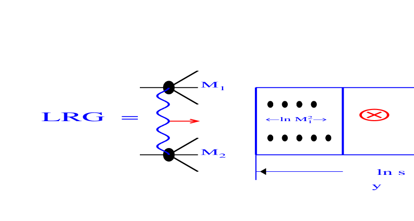
Figure 1: Lego-plot for double Pomeron Higgs production process.

The main idea behind all calculations, starting from the Bialas-Landshoff paper [1], is to describe the reactions of Eq. (1) and Eq. (2) as a double Pomeron (DP) Higgs production ( see Fig.2 ) . In Fig.2, the Pomerons are the so–called “soft” Pomerons for which one uses the phenomenological Donnachie-Landshoff form ( see Ref. [7] ), while the vertex $\gamma$ can be calculated in perturbative QCD.

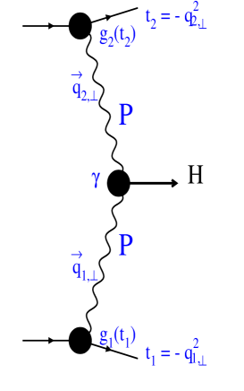
Figure 2: Double Pomeron Higgs production process.

We can demonstrate the problems and uncertainties of such kind of approach by considering the simplest pQCD diagram for the double Pomeron Higgs production ( DPHP ) (see Fig.3-a). This diagram leads to the amplitude

$$M(qq\rightarrow qHq)=\frac{2}{9}\,2\,g_{H}\int\frac{d^{2}Q_{\perp}}{Q^{2}_{\perp}\,Q^{2}_{1,\perp}\,Q^{2}_{2,\perp}}\,4\,\alpha_{S}(Q^{2}_{\perp})\,(\vec{Q}_{1,\perp}\,\cdot\,\vec{Q}_{2,\perp})\,,$$ (4)

where $g_{H}$ is the Higgs coupling that has been evaluated in perturbative QCD [8]. For the reaction of Eq. (1), $|t_{1}|=|\vec{Q}_{\perp}-\vec{Q}_{1,\perp}|\,\approx\,|t_{2}|=|\vec{Q}_{\perp}-\vec{Q}_{2,\perp}|\,\approx\,2/B_{el}$ and therefore,

$$M(q+q\rightarrow q+H+q)\,\propto\,\int\frac{d^{2}Q_{\perp}}{Q^{4}_{\perp}}.$$ (5)

Eq. (5) has an infrared divergence which is regularized by the size of the colliding hadrons. In other words, one can see that already the simplest diagrams show that the DP Higgs production is, in a sense, a “soft” process. Taking into account the emission of extra gluons denoted in Fig.3-b as Pomeron builders, we recover the exchange of the “soft” Pomerons.

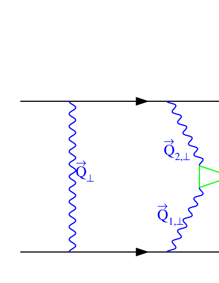
Fig. 3-a	Fig.3-b

Figure 3: Double Pomeron Higgs production in the Born approximation (Fig. 3-a ) and in leading log approximation (Fig. 3-b ) of pQCD.

Nevertheless, the emission vertex for the Higgs boson can still be calculated in pQCD since the typical distances inside the quark triangle in fig.3-a are rather short $\propto 1/M_{T}$, where $M_{T}$ is the mass of t-quark. The coupling $g_{H}$ has been evaluated in Ref.[8] and is given by

$$g^{2}_{H}\,=\,\sqrt{2}\ G_{F}\ \alpha^{2}_{S}(M^{2}_{H})\ N^{2}/9\pi^{2},$$ (6)

where $N$ is a function of the ratio $M_{T}/M_{H}$ which was calculated in Refs. [8, 3].

In this paper we consider an alternative approach to DPHP, in which we estimate the value of the cross section from non–perturbative QCD. In section 2 we review a non–perturbative method suggested by Shifman, Vainshtein and Zakharov [9] for the evaluation of the coupling of the Higgs boson to hadrons; it is valid if the mass of the Higgs is smaller than the mass of the top quark. In section 3 we develop a method of obtaining the DPHP cross section using the approach of Ref. [9]. The problem of survival of large rapidity gaps (LRG) will be discussed in section 4. We conclude in section 5 with discussion of our results and of the uncertainties inherent to our approach.

2 The coupling of Higgs boson to hadrons in
non-perturbative QCD

To evaluate the non–perturbative coupling of the Higgs boson to hadrons, we need to have a closer look at the properties of the energy–momentum tensor in QCD. The trace of this tensor is given by

$$\Theta^{\alpha}_{\alpha}={\beta(g)\over 2g}G^{\alpha\beta a}G^{a}_{\alpha\beta}+\sum_{l=u,d,s}m_{l}(1+\gamma_{m_{l}})\bar{q_{l}}q_{l}+\sum_{h=c,b,t}m_{h}(1+\gamma_{m_{h}})\bar{Q_{h}}Q_{h},$$ (7)

where $\gamma_{m}$ are the anomalous dimensions; in the following we will assume that the current quark masses are redefined as $(1+\gamma_{m})m$. The appearance of the scalar gluon operator in (7) is the consequence of scale anomaly [10], [11]. The QCD beta function can be written as

$$\beta(g)=-b{g^{3}\over 16\pi^{2}}+...,\ b=9-{2\over 3}n_{h},$$ (8)

where $n_{h}$ is the number of heavy flavors ($c,b,..$). Since there is no valence heavy quarks inside light hadrons, at scales $Q^{2}<4m_{h}^{2}$ one expects decoupling of heavy flavors. This decoupling was consistently treated in the framework of the heavy-quark expansion [9]; to order $1/m_{h}$, only the triangle graph with external gluon lines contributes. Explicit calculation shows [9] that the heavy-quark terms transform in the piece of the anomalous gluonic part of $\Theta^{\alpha}_{\alpha}$:

$$\sum_{h}m_{h}\bar{Q_{h}}Q_{h}\to-{2\over 3}\ n_{h}\ {g^{2}\over 32\pi^{2}}G^{\alpha\beta a}G^{a}_{\alpha\beta}+...$$ (9)

It is immediate to see from (9), (7) and (8) that the heavy-quark terms indeed cancel the part of anomalous gluonic term associated with heavy flavors, so that the matrix element of the energy–momentum tensor can be rewritten in the form

$$\Theta^{\alpha}_{\alpha}={\tilde{\beta}(g)\over 2g}G^{\alpha\beta a}G^{a}_{\alpha\beta}+\sum_{l=u,d,s}m_{l}\bar{q_{l}}q_{l},$$ (10)

where heavy quarks do not appear at all; the beta function in (3.10) includes the contributions of light flavors only:

$$\tilde{\beta}(g)=-9{g^{3}\over 16\pi^{2}}+...$$ (11)

Because the mass of the Higgs boson $M_{H}$ is presumably large, its coupling to hadrons involves the knowledge of hadronic matrix elements at the scale $Q^{2}\sim M_{H}^{2}$, at which the heavy quarks in general are not expected to decouple. However, if the Higgs boson mass $M_{H}$ is smaller than the mass of the top quark $M_{T}$, one can still perform expansion in the ratio $M_{H}/M_{T}$; we expect this to be a reasonable procedure if $M_{H}\leq 100$ GeV. In this case, one finds

$$M_{T}\bar{t}t\to-{2\over 3}\ {g^{2}\over 32\pi^{2}}G^{\alpha\beta a}G^{a}_{\alpha\beta}+...$$ (12)

Since the mass of the hadron is defined as the forward matrix element of the energy–momentum tensor, the expression Eq. (12) leads to the following Yukawa vertex for the coupling of a Higgs boson to the hadron:

$$2^{\frac{1}{4}}G^{\frac{1}{2}}_{F}\cdot H\phi^{2}_{h}\,\cdot\,\langle h|M_{T}\bar{t}t|h\rangle\,\,=\,\,2^{\frac{1}{4}}G^{\frac{1}{2}}_{F}\cdot H\phi^{2}_{h}\,\cdot\,\frac{2M^{2}}{27}\,\,;$$ (13)

this relation is valid in the chiral limit of massless light quarks (see Eq. (10)); $M_{T}$ is the mass of the heavy quark and $M$ is the hadron mass. We put the number of light quarks $N_{F}=3$ and the number of colors $N_{c}=3$; $\phi_{h}$ and $H$ are hadron and Higgs operators. Note that, as a consequence of scale anomaly, Eq. (13) does not have an explicit dependence on the coupling $\alpha_{s}$.

3 Estimates for double Pomeron Higgs production cross sections

3.1 General formulae for double Pomeron Higgs production

The amplitude for Higgs production in the Pomeron approach is given by ( see for example Refs.[1, 12])

$$M(h+h\rightarrow h+H+h)\,\,=\,\,g_{1}(t_{1})\,\cdot\,g_{2}(t_{2})\,\cdot\,\gamma(t_{1},t_{2})\,\cdot\,\eta_{+}(t_{2})\eta_{+}(t_{1})\,\cdot\,\left(\,\frac{s}{s_{2}}\right)^{\alpha_{P}(t_{2})}\,\cdot\,\left(\,\frac{s}{s_{1}}\right)^{\alpha_{P}(t_{1})}\,\,,$$ (14)

where $s_{1}=(P_{1}+q_{1})^{2}$ and $s_{2}=(P_{2}+q_{1})^{2}$ ( $P_{1,2}$ are momenta of incoming hadrons ); $\eta_{+}(t_{i})$ is a signature factor, which for the Pomeron is

$$\eta_{+}(t_{i})\,\,\,=\,\,\,i+tan^{-1}\left(\frac{\pi\alpha_{P}(t_{i})}{2}\right)\,\,,$$ (15)

where $\alpha_{P}(t)$ is the Pomeron trajectory, $\alpha_{P}(t)=1+\Delta_{P}+\alpha^{\prime}_{P}\,\,t$, with $\Delta_{P}\approx 0.08$ [7]; all other notations are evident from Fig.2.

The cross section for DPHP in the central rapidity region ($y_{H}=0$, where $y_{h}$ is the rapidity of the produced Higgs boson) can be written down as

$$\frac{d\sigma}{dy_{H}dt_{1}dt_{2}}|_{y_{H}=0}\,\,=$$ (16)

$$\,\,\frac{1}{2s}|M(h+h\rightarrow h+H+h)|^{2}\prod_{i=1,2}\,\cdot\,\frac{d^{3}P^{\prime}_{i}}{(2\pi)^{3}2P^{\prime}_{i,0}}\,\cdot\frac{d^{2}p_{H,\perp}}{2(2\pi)^{3}}\,\cdot\,(2\pi)^{4}\,\delta^{(4)}(P_{1}+P_{2}-P^{\prime}_{1}-P^{\prime}_{2}-p_{H})\,\,$$

where $P^{\prime}_{i}$ are momenta of recoil hadrons, while $p_{H}$ is the momentum of the produced Higgs boson.

Performing all integrations and recalling that $s_{1}\cdot s_{2}=M^{2}_{H}\cdot s$ we obtain

$$\frac{d\sigma}{dy_{H}dt_{1}dt_{2}}|_{y_{H}=0}\,\,=\,\,\frac{2\,\,g^{2}_{1}(t_{1})\cdot g^{2}_{2}(t_{2})\cdot\gamma^{2}(t_{1},t_{2})}{\pi(16\pi)^{2}}\,\cdot\,\left(\frac{s}{M^{2}_{H}}\right)^{2\,\Delta_{P}}\,\cdot e^{\alpha^{\prime}_{P}\,\ln(s/M^{2}_{H})\,[t_{1}+t_{2}]}\,\,.$$ (17)

We will assume that $\gamma(t_{1},t_{2})$ is a smooth function of $t_{1}$ and $t_{2}$ in comparison with $g_{1}(t_{1})$ and $g_{2}(t_{2})$. Indeed, the t-dependence of $g_{i}$ is related to the quark distribution inside the hadron while the t-dependence of $\gamma$ is determined by the mean transverse of gluon inside the Pomeron. The typical scale for this momentum is $1/\alpha_{P}\,\approx\,4\ GeV^{2}$ which is much larger than the typical momentum of a quark in a hadron ( $\approx\,\,0.1\ GeV^{2}$ ).

Using this assumption together with the simplest Gaussian parameterization for the vertex $g_{i}(t_{i})=g_{i}(0)\,\,exp(-R^{2}_{0}\,|t_{i}|)$ we obtain

$$\frac{d\sigma}{dy_{H}}|_{y_{H}=0}\,\,\,=\,\,\,\frac{8g^{2}_{1}(0)\,\,g^{2}_{2}(0)}{\pi[16\pi B_{el}(s/M^{2}_{H})]^{2}}\,\cdot\,\gamma^{2}(t_{1}=0,t_{2}=0)\,\cdot\,\left(\,\frac{s}{M^{2}_{H}}\,\right)^{2\,\Delta_{P}}\,\,.$$ (18)

Recalling now the well–known relation between the total and elastic cross sections for the one Pomeron exchange, namely,

$$R_{el}(s)\,\,=\,\,\frac{\sigma_{el}(s)}{\sigma_{tot}(s)}\,\,=\,\,\frac{g_{1}(0)g_{2}(0)}{16\pi B_{el}(s)}\,\,\left(\,\frac{s}{s_{0}}\,\right)^{\Delta_{P}}\,\,;$$ (19)

where $B_{el}=4\,R^{2}_{0}+2\alpha^{\prime}_{P}\,\ln s$, one can derive

$$\frac{d\sigma}{dy_{H}}|_{y_{H}=0}\,\,\,=\,\,\,\gamma^{2}(t_{1}=0,t_{2}=0)\,\times\,\frac{8}{\pi}\,\times\,R_{el}^{2}\left(\,\frac{s}{M^{2}_{H}}\,s_{0}\,\right)\,\,.$$ (20)

There is only one unknown factor in Eq. (20), namely, $\gamma^{2}(t_{1}=0,t_{2}=0)$. In the next subsection we present the estimates for this factor using the non-perturbative approach that has been discussed in the section 2.

3.2 The production vertex $\gamma(t_{1}=0,t_{2}=0)$

Our estimate of $\gamma(t_{1}=0,t_{2}=0)$ consists of two steps:

1. For positive values of $t_{1}=t_{2}=m^{2}_{glueball}$ we can obtain $\gamma(t_{1}=m^{2}_{glueball},t_{2}=m^{2}_{glueball})$ from Eq. (13);

2. Using Eq. (14) we can make the analytic continuation to the region $t_{1}<0$ and $t_{2}<0$, which corresponds to the scattering process.

We will assume that there exists a tensor $2^{++}$ glueball which lies on the Pomeron trajectory, namely, that its mass satisfies the following relation:

$$\alpha_{P}(t=m^{2}_{glueball})\,\,\,=\,\,\,1\,+\,\Delta\,+\,\alpha^{\prime}_{P}(0)\,m^{2}_{glueball}\,\,\,=\,\,\,2\,\,.$$ (21)

There is no undisputed experimental evidence for such a meson but lattice calculations give for its mass $m_{glueball}=2.4$ GeV [13]. This mass is a little bit higher than can be expected from Eq. (21) with the experimental $\alpha^{\prime}_{P}(0)=0.25\,GeV^{-2}$ [7]. On the other hand, it is possible to describe experimental data using a smaller value of $\alpha^{\prime}_{P}(0)\approx 0.17\,GeV^{-2}$ which is needed to satisfy Eq. (21) with $m_{glueball}=2.4\ GeV$, assuming the presence of substantial shadowing corrections [14].

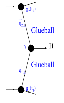
Figure 4: Higgs emission from glueball.

For the diagram in Fig.4 the vertex $\gamma_{glueball}$ can be easily evaluated from Eq. (13); it is equal to

$$\gamma_{glueball}\,\,\,=\,\,\,2^{\frac{1}{4}}\,\,G^{\frac{1}{2}}_{F}\,\,\frac{2\,m^{2}_{glueball}}{27}\,\,.$$ (22)

One can see that Eq. (14) leads to the contribution described by Fig.4. Indeed, for $t_{i}\,\longrightarrow\,m^{2}_{glueball}$

$$\eta_{+}(t_{i})\,\,\longrightarrow\,\,\frac{2}{\pi\,\,\alpha^{\prime}_{P}\,\left(\,m^{2}_{glueball}\,\,-\,\,t_{i}\,\right)}\,\,.$$ (23)

(A more detailed discussion of the analytic properties of the Reggeon exchange can be found in Ref. [15]). Using Eq. (23) and comparing Eq. (14) with the diagram of Fig.4, we conclude that

$$\gamma(t_{1}=m^{2}_{glueball},t_{2}=m^{2}_{glueball})\,\,\,=\,\,\frac{\pi}{2}\,\,\alpha^{\prime}_{P}(0)\,\,\gamma_{glueball}\,\,.$$ (24)

The reggeon approach cannot tell us anything on the relation between $\gamma(t_{1}=m^{2}_{glueball},t_{2}=m^{2}_{glueball}$ and $\gamma(t_{1}=0,t_{2}=0)$. The only thing that we can claim is that the signature factor takes into account the steepest part of $t$-behavior. Therefore, in the next subsection we will assume that

$$\gamma(t_{1}=m^{2}_{glueball},t_{2}=m^{2}_{glueball})\,\,\,=\,\,\gamma(t_{1}=0,t_{2}=0)\,\,;$$ (25)

this is an extreme assumption which can be used to obtain an upper bound on the cross section. Uncertainties related to this and other assumptions we make will be discussed in detail in section 3.4 and in the summary, section 5.

3.3 The magnitude of the cross section

Using Eq. (22),Eq. (24) and Eq. (25) we can rewrite Eq. (20) in the simple form

$$\frac{d\sigma}{dy_{H}}|_{y_{H}=0}\,\,\,=\,\,\,2\,\pi\,\left(\alpha^{\prime}_{P}\,m^{2}_{glueball}\right)^{2}\times\frac{4\,\sqrt{2}\,\,G_{F}}{27^{2}}\times\,R^{2}\left(\,\frac{s}{M^{2}_{H}}\,s_{0}\,\right)\,\,.$$ (26)

For $M_{H}=100\ GeV$, the factor $S/M^{2}_{H}\cdot s_{0}$ is equal to $400\ GeV^{2}$ for $s_{0}=1\ GeV^{2}$. Therefore, we can take $R_{el}\simeq 0.175$ ( see Fig.5 ) for the Tevatron energies. Eq. (26) leads to

$$\frac{d\sigma}{dy_{H}}|_{y_{H}=0}(M_{h}=100\,\,GeV,\sqrt{s}=1800\,GeV)\,\,=\,\,6.4\,{\rm pbarn}\,\,,$$ (27)

This is a very large number, especially if we recall that the total inclusive cross section for Higgs production in perturbation theory is on the order of $1$ pbarn [16]. However this estimate does not yet contain the suppression due to the (small) probability of the rapidity gap survival, which will be discussed in section 4, where we present our final results. Since $R_{el}$ grows with energy, $R_{el}\,\,\propto\,\,s^{\Delta}$ we expect that the cross section at the LHC energy is approximately 2 times larger than the one in Eq. (27).

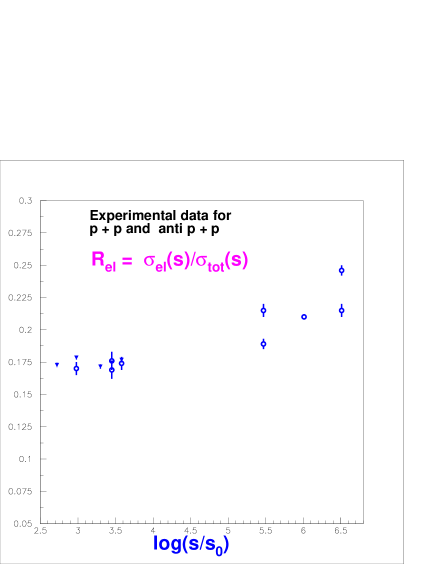
Figure 5: Experimental data for the ratio $R_{el}(s)=\sigma_{el}(s)/\sigma_{tot}(s)$. $s_{0}$ = $1\,GeV^{2}$ and the log is taken on base 10.

3.4 Uncertainties of our estimates

1. Let us start with the value of $R_{el}$. We took it from the experimental data, but we nevertheless have two uncertainties associated with it. First, Eq. (19) is written for one Pomeron exchange while in experimental data at $\sqrt{s}\approx\,20\,GeV$ we have about 30% contamination from the secondary Reggeons [7]. If we try to extract the one Pomeron exchange from the data, it reduces the value of cross section for DPHP by 1.7 times. Therefore, the value for the cross section can be about $3.8\ pbarn$ rather than Eq. (27). The second uncertainty in evaluation of $R_{el}$ is the value of $s_{0}$; even though $s_{0}=1\,GeV$ appears in all phenomenological approaches [7, 14], we have no theoretical argument for the value of $s_{0}$. However, since the ratio $R_{el}$ in Fig.5 is a rather smooth function of energy we do not expect that the uncertainty in the value of $s_{0}$ can introduce a large error.

2. We can take into account also the reactions of Eq. (2) and Eq. (3). In Eq. (26) we would then have to substitute

$$R_{el}\,\,\longrightarrow\,\,R_{D}=R_{el}+\frac{\sigma^{DD}(s)}{\sigma_{tot}}\,\,,$$ (28)

where $\sigma^{DD}$ is the cross section of the double diffraction dissociation. Unfortunately, we do not have conclusive data on this cross section. However, recent CDF measurements [17] show that this cross section could be rather large ( about 4.7 mb at the Tevatron energy).

3. The principle uncertainty, however, is associated with the continuation from $t=m^{2}_{glueball}$ to $t=0$. This is a question which at present can only be addressed in the framework of different models. For example, in Veneziano model [18] instead of $\eta_{+}(t)$ (see Eq. (15) ) a new factor appears, namely

$$\eta^{V}_{+}(t_{i})=\Gamma(2-\alpha_{P}(t_{i}))\,e^{i\frac{\pi\alpha_{P}(t_{i})}{2}}\,\,.$$ (29)

Eq. (29) does not give the factor of $\pi/2$ in Eq. (24) and, therefore, decreases the value of the cross section given by Eq. (26) by a factor of 2.5. We will return to the discussion of the analytic continuation in the summary section.

4. As we have discussed in section 2, we can evaluate the value of $\gamma(t_{1}=m^{2}_{glueball},t_{2}=m^{2}_{glueball})=\gamma_{glueball}$ only if $M_{H}/M_{T}<1$. The accuracy of Eq. (22) is $O(M^{2}_{H}/M^{2}_{T})$ and we thus believe that Eq. (22) gives a reasonable estimate of $\gamma_{glueball}$ for Higgs meson with $M_{H}\leq 100\,GeV$.

4 Survival of large rapidity gaps

As has been discussed intensively during the past decade (see Refs.[19, 20, 21, 22, 23, 24, 25, 26, 27, 28, 29]), the cross section of Eq. (26) has to be multiplied by a factor $S^{2}_{spect}$, which is the survival probability of large rapidity gap (LRG) processes. The “experimental” cross section is therefore given by

$${\frac{d\sigma(pp\rightarrow ppH)}{dy}}|_{y=0}\,\,=\,\,S^{2}_{spect}\frac{d\sigma_{P}(pp\rightarrow ppH)}{dy}|_{y=0}\,\,.$$ (30)

Here, ${d\sigma_{P}(pp\rightarrow ppH)}/{dy}$ denotes the cross section calculated in Eq. (26). The factor $S^{2}_{spect}$ has a very simple meaning – it is a probability of the absence of inelastic interactions of the spectators which could produce hadrons inside the LRG. We have rather poor theoretical control of the value of the survival probability; this fact reflects the lack of knowledge of the “soft” physics stemming from non-perturbative QCD. Different models exist, leading to the values about $S^{2}_{spect}\,\,\approx\,\,10^{-1}$ at the Tevatron energies. For double Pomeron processes, this quantity has been discussed in Ref [30]. The result of this analysis is that the value of the survival probability for double Pomeron production is almost the same as for “hard” dijet production with LRG between them. Fortunately, the value of $S^{2}_{spect}$ has been measured [31], and is equal to 0.07 for the highest Tevatron energy.

Multiplying Eq. (27) by $S^{2}_{spect}$ = 0.07 and taking into account suppression due to the factor of Eq. (29), we obtain

$$\frac{d\sigma}{dy_{H}}|_{y_{H}=0}(M_{h}=100\,\,GeV,\sqrt{s}=1800\,GeV)\,\,=\,\,0.2\,{\rm pbarn}.$$ (31)

This estimate is not our final result yet, since we still have to correct it by the additional suppression factor $S^{2}_{par}$ which describes the probability of the absence of the parasite gluon emission around the Higgs production vertex (see Fig.4-b) [6]. As was argued in Ref.[6],

$$S^{2}_{par}\,\,=\,\,e^{-<N_{G}(\Delta y=\ln(M^{2}_{H}/s_{0}))>}\,\,,$$ (32)

with

$$<N_{G}(\Delta y=\ln(M^{2}_{H}/s_{0}))>\,\,\,=\,\,\,\frac{N_{hadrons}(\Delta y=\ln(M^{2}_{H}/s_{0}))}{N_{hadrons}(one\,\,\,minijet)}\,\,\approx\,\,\,2\,\div\,4\,\,.$$ (33)

It gives $S^{2}_{par}=0.14\,\div\,0.014$.

The appearance of this factor can be illustrated by the following argument: one of the most important differences between the diagrams of Fig.2 and in Fig.4 is the fact that the Pomeron exchange is almost purely imaginary while the glueball exchange leads to the real amplitude. Imaginary amplitude describes the production of particles and the Pomeron is associated with the inelastic process with large multiplicity. Therefore, normally, in a large rapidity region $\Delta y=\ln(M^{2}_{H}/s_{0})$ we expect to see a large number of produced particles while in Fig.2 we require that only one Higgs boson is produced. Therefore, it seems reasonable to expect a suppression for the double–diffractive Higgs production, and this suppression can be described by Eq. (32) and Eq. (33).

Finally, for the Tevatron energy we expect

$$\frac{d\sigma(pp\rightarrow ppH)}{dy}|_{y=0}\left(\sqrt{s}\,=\,\,1.8\,TeV\right)\,\, = \,\,S^{2}_{spect}\,\times\,S^{2}_{par}\,\times\,\frac{d\sigma_{P}(pp\rightarrow ppH)}{dy}|_{y=0}$$

$$= \,\,\left(\,0.0038\,\div\,0.028\,\right)\,{\rm pbarn}$$ (34)

Extrapolating to the LHC energy, we have two effects that work in different directions: the rise of the Pomeron contribution and the decrease of the $S^{2}_{spect}$ with energy. From Ref. [30] we expect that $S^{2}_{spect}(\sqrt{s}\,\,=\,\,16\,TeV)/S^{2}_{spect}(\sqrt{s}\,\,=\,\,1.8\,TeV)\,\,\approx\,\,0.7$ while the rise of the Pomeron exchange leads to an extra factor of 2 in Eq. (34). Therefore, our final estimate for the LHC is

$$\frac{d\sigma(pp\rightarrow ppH)}{dy}|_{y=0}\left(\,\sqrt{s}\,=\,16\,TeV\,\right)\,\, = \,\,S^{2}_{spect}\,\times\,S^{2}_{par}\,\times\,\frac{d\sigma_{P}(pp\rightarrow ppH)}{dy}|_{y=0}\,$$ (35)

$$= \,\,\left(\,0.0015\,\div\,0.042\,\right)\,{\rm pbarn}\,\,.$$

Eq. (34) and Eq. (35) give significantly larger (by about $5$ times) larger cross sections than expected for double–diffractive production in pQCD [33]. However, Ref. [6] contains an estimate of the upper bound on double Pomeron Higgs production in pQCD obtained by choosing the largest possible value for $S^{2}_{par}$ ( see Eq. (33) ). This upper bound appears to be about 7 times larger than the highest value in Eq. (34).

5 Summary and discussion

The approach suggested in this paper is based entirely on non-perturbative QCD. We believe that such an approach is logically justified for diffractive Higgs production since even pQCD calculations show that this is, to large extent, a “soft” process (see Eq. (5) and the following discussion). However, just because of this, we have to stress again that the accuracy of our calculation is not very good. We feel, however, that our results support the idea [6] that in pQCD approach to diffractive Higgs production the running QCD coupling has to be taken at the “soft” scale $Q^{2}\sim 1\ {\rm GeV}^{2}$. As was argued in Ref.[6], in BLM prescription [32] of taking into account the running QCD coupling one can insert the quark bubbles only in the $t$-channel gluon lines in Fig. 3. Therefore, the running QCD coupling depends on the transverse momenta of these gluons, and they are determined by the “soft” scale. The Eq. (13) indeed does not depend on the QCD coupling, demonstrating the non-perturbative, “soft” character of the discussed process.

We obtain quite large values for the cross section of the diffractive Higgs production – after integration over the Higgs rapidity $y$ in Eq. (34) and Eq. (35) we get

$$\sigma(pp\rightarrow ppH)\left(\sqrt{s}\,=\,\,1.8\,TeV\right)\,\,=\,\,0.019\,\div\,0.14\,\,\,\,\,{\rm pbarn}\,\,.$$ (36)

and

$$\sigma(pp\rightarrow ppH)\left(\sqrt{s}\,=\,\,16\,TeV\right)\,\,=\,\,0.01\,\div\,0.27\,\,\,\,\,{\rm pbarn}\,\,.$$ (37)

Comparing our estimates with the ones based on pQCD [1, 2, 3, 4, 5, 6] we conclude that the lowest of our values of the cross section of double Pomeron Higgs production is about the same as the highest one in the pQCD approach. However, both our approach and the pQCD one are suffering from large uncertainties, stemming from the analytical continuation in our approach and from the survival probability of rapidity gap and the absence of “parasite emission” $S^{2}_{par}$ in pQCD.

Let us point out that Eq. (36) shows that the double Pomeron Higgs production constitutes a substantial part of the total inclusive Higgs production. Moreover, our calculations lead to an additional contribution to the inclusive cross section which is shown in Fig.6.

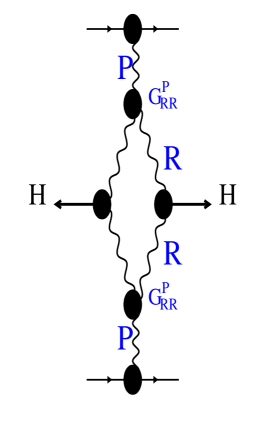
Figure 6: Mueller diagram [35] for “soft” inclusive Higgs production.

(Note that the triple Pomeron interaction gives a very small contribution to the process in Fig. 6 due to the small real part in the Pomeron exchange [36].) Using the same approach as in derivation of Eq. (17) we obtain

$$\frac{d\sigma_{incl}(pp\longrightarrow H+X)}{dy}|_{y_{H}=0}\,\,\,\,=\,\,\,\,\gamma^{2}_{R}(t_{1}=0,t_{2}=0)\,\,\frac{2g_{1}(0)g_{2}(0)(G^{P}_{RR})^{2}}{\pi(16\pi B_{R})^{2}}\,\,\,\frac{1}{\Delta^{2}_{R}}\,\,\left(\,\frac{s}{M^{2}_{H}}\,\right)^{\Delta_{P}}\,\,,$$ (38)

where $\Delta_{R}\approx 0.5$. As a first approximation we can take ( see Eq. (24) )

$$\gamma_{R}(t_{1}=0,t_{2}=0)\,\,\,=\,\,\,\frac{\pi}{2}\,2^{\frac{1}{4}}G^{\frac{1}{2}}\,\,\frac{2\alpha^{\prime}_{R}\,m^{2}_{f}}{27}\,\,$$ (39)

where $m_{f}$ is the mass of the $f$ - meson which is the first resonance on the secondary Reggeon trajectory, and $\alpha^{\prime}_{R}\,m^{2}_{f}=1.5$. Substituting Eq. (39) in Eq. (38) we obtain

$$\frac{d\sigma_{incl}(pp\longrightarrow H+X)}{dy}|_{y_{H}=0}\,\,=\,\ \frac{(G^{P}_{RR})^{2}}{8\,B_{R}}\,\times\,\frac{B_{R}}{B_{el}}\,\times\,2^{\frac{1}{2}}\,G_{F}\,\frac{1}{3}\,\times\,R\left(\,\frac{s}{M^{2}_{H}}\,s_{0}\,\right)\,\,.$$ (40)

Eq. (40) gives

$$\frac{d\sigma_{incl}(pp\longrightarrow H+X)}{dy}|_{y_{H}=0}\,\,=\,\ \,\,\left(\frac{G^{P}_{RR}}{g}\right)^{2}\,\,\,3.4\,10^{-7}\,mb\,\,$$ (41)

which does not yet contain the suppression arising from the analytical continuation. We take this suppression into account by multiplying Eq. (41) by factor $S^{2}_{par}=0.14-0.014$. Unfortunately, we do not know the value for the ratio $G^{P}_{RR}/g$. In the triple Pomeron parameterization of the cross section of diffractive dissociation in hadron reactions [37] this ratio changes from 1 to 0. For $G^{P}_{RR}/g=1$ we get for the “soft” inclusive cross section the value of $43\div 430\,{\rm pbarn}$. On the other hand, taking Field and Fox value [37] for this ratio we obtain a much smaller, but still very sizeable value of $0.43\,\div\,4.28\,{\rm pbarn}$. It is thus clear that the evaluation of the “soft” contribution to the inclusive Higgs production is plagued by large uncertainties; however, it might be bigger than the pQCD one [16].

We hope that this paper will help to look at diffractive Higgs production from a different viewpoint, and will stimulate a much needed further work. To our surprise, despite the very different non–perturbative method used here, our estimates for the double–diffractive production turn out to be not that far from the pQCD calculation [33] ( the average is about $5$ times larger ). It adds some confidence in both approaches and gives us a hope that one will be able to perform a reliable calculation in the nearest future.

Acknowledgments: We are very grateful to Mike Albrow, Andrew Brandt, Al Mueller and all participants of the working group “Diffraction physics and color coherence” at QCD and Weak Boson Physics Workshop in preparation for Run II at the Fermilab Tevatron for stimulating discussions of Higgs production and encouraging criticism. We thank Stan Brodsky, Asher Gotsman, Valery Khoze, Larry McLerran, Uri Maor and Misha Ryskin for fruitful discussions on the subject. E.L. thanks the Fermilab theory department for creative atmosphere and hospitality during his stay when this paper was being written.

The work of D.K. was supported by the US Department of Energy (Contract # DE-AC02-98CH10886) and RIKEN. The research of E.L. was supported in part by the Israel Science Foundation, founded by the Israeli Academy of Science and Humanities, and BSF # 9800276.

References

- [1] A. Bialas and P.V. Landshoff, Phys. Lett. B256 (1991) 540.
- [2] B. Müller and A.J. Schramm, Nucl. Phys. A523 (1991) 677.
- [3] J-R Cudell and O.F. Hernandez, Nucl. Phys. B471 (1996) 471.
- [4] V. Barger, R.J.N.Phillips and D.Zeppenfeld, Phys. Lett. B346 (1995) 106.
- [5] A.D. Martin, M.G. Ryskin and V.A. Khoze, Phys.Rev. D56 (1997) 5867; Phys.Lett. B401 (1997) 330.
- [6] E. Levin, talk at “Physics at runII WS”, WGVI,Fermilab,January-December 1999, BNL-NT-99/9,TAUP-2615-99 hep-ph/9912403.
- [7] A. Donnachie and P.V. Landshoff, Nucl. Phys. B244 (1984) 322, Nucl. Phys. B267 (1986) 690, Phys. Lett. B296 (1992) 227, Z. Phys. C61 (1994) 139.
- [8] S. Dawson,Nucl. Phys. B359 (1991) 283; A. Djouadi, M. Spira and P. Zerwas, Phys. Lett. B264 (1991) 440.
- [9] M.A. Shifman, A.I. Vainshtein and V.I. Zakharov, Phys. Lett. B78 (1978) 443.
-
[10]
J. Ellis, Nucl. Phys. B22 (1970) 478;
R.J. Crewther, Phys. Lett. B33 (1970) 305;
R.J. Crewther, Phys. Rev. Lett. 28 (1972) 1421;
M.S. Chanowitz and J. Ellis, Phys. Lett. B40 (1972) 397; Phys. Rev. D7 (1973) 2490. -
[11]
J. Collins, A. Duncan and S.D. Joglekar, Phys. Rev. D16 (1977) 438;
N.K. Nielsen, Nucl. Phys. B120 (1977) 212. - [12] E. Gotsman, E. Levin and U. Maor, Phys.Lett. B353 (1995) 526.
- [13] C.J. Morningstar and M. Peardon, Phys.Rev. D60 (1999) 034509.
-
[14]
A.B. Kaidalov and K. A. Ter Martirosyan, Phys. Let. B117
(1982)
247;
A.B. Kaidalov, K. A. Ter Martirosyan and Yu. M. Shabelsky,Sov. J. Nucl. Phys. 43 (1986) 822;
A. Capella, U. Sukhatme, C-I Tan anf J. Tran Tranh Van, Phys. Rept. 236 (1994) 225 and references therein;
E. Gotsman,E. Levin and U. Maor, Phys. Lett. B452 (1999) 287, Phys. Rev. D49 (1994) 4321, Phys. Lett. B304 (1993) 199, Z. Phys. C57 (1993) 672. -
[15]
P.D.R. Collins,“An introduction to Regge theory and high energy
physics”,Cambridge U.P.,1977;
The collection of the best original papers on Reggeon approach can be found in: “Regge Theory of low Hadronic Interaction”,ed. L. Caneschi, North-Holland, 1986;
E.Levin, “Everything about Reggeons. Part I: Reggeons in “Soft” Interactions”,Academic Training Program lecture, DESY, 1996, TAUP-246-97,DESY-97-213,hep-ph/9710596. - [16] A. Stange, W. Marciano and S. Willenbrock, Phys. Rev. D49 (1994) 1354.
- [17] M.E. Convery, talk at “Physics at runII WS”, WGVI,Fermilab, January-December 1999.
- [18] G. Veneziano, Nuovo Cimento A57 (1968) 190.
- [19] Yu.L. Dokshitzer, V. Khoze and S.I. Troyan, Sov.J.Nucl.Phys. 46 (1987) 116.
- [20] Yu.L. Dokshitzer, V.A. Khoze and T. Sjostrand, Phys.Lett. B274 (1992) 116.
- [21] J.D. Bjorken, Phys.Rev. D45 (1992) 4077; D47 ( 1993 ) 101.
- [22] A.D. Martin, M.G. Ryskin and V.A. Khoze, Phys.Rev. D56 (1997) 5867; Phys. Lett B401 (1997) 330.
- [23] G. Oderda and G. Steman, Phys.Rev. Lett. 81 (1998) 359; Talk at ISMD’99, Providence,RI, 9-13 Aug 1999, hep-ph/9910414;
- [24] E. Gotsman, E. Levin and U. Maor, Phys.Rev. D48 (1993) 2097; Nucl.Phys. B493 (1997) 354; Phys. Lett. B438 (1998) 229.
- [25] E. Gotsman, E. Levin and U. Maor, Phys.Rev. D60 (1999) 094011; Phys. Lett. B438 (1998) B452 (1999) 387, B438 (1998) 229.
- [26] R.S. Fletcher,Phys.Rev. D48 (1993) 5162; Phys.Lett. B320 (1994) 373.
- [27] A. Rostovtsev and M.G. Ryskin, Phys. Lett. B390 (1997) 375 ).
- [28] E. Levin, A.D. Martin and M.G. Ryskin. J.Phys. G25 (1999) 1507.
- [29] E. Levin, talk at “Physics at runII WS”, WGVI,Fermilab, January-December 1999, BNL-NT-99/10, TAUP -2614-99,hep-ph/9912402.
- [30] E. Gotsman, E. Levin and U. Maor,Phys.Lett. B353 (1995) 526.
-
[31]
A. Brandt,“Probing Hard Color-Singlet Exchange”, talk at the
Workshop on Small-x and Diffractive Physics, Sep.
1998, Fermilab and references therein;
B. Abatt et al., Phys.Lett. B440 (1998) 189. - [32] S.J. Brodsky, P. Lepage and P. B. Mackenzie, Phys. Rev. D28 (1983) 228.
- [33] V.A. Khoze, A.D. Martin and M.G. Ryskin, DTP/00/08, hep-ph/0002072.
-
[34]
D. Kharzeev and E. Levin, hep-ph/9912216; Nucl. Phys. B, in press;
E.V. Shuryak, hep-ph/0001189. - [35] A.H. Mueller, Phys.Rev. D2 (1970) 2963, D4 (1971) 150.
- [36] E. Gotsman, E. Levin and U. Maor,Phys.Lett. B406 (1997) 89.
-
[37]
R.D. Field and G.C. Fox, Nucl. Phys. B80 (1974) 367;
A. Donnachie and P.V. Landshoff, Nucl.Phys. B244 (1984) 322; B303 (1988) 634; Phys. Lett. B191 (1987) 309;
UA8 Collaboration, A. Brandt et al., Nucl. Phys. B514 (1988) 3;
K. Goulianos and J. Montanha, Phys.Rev. D59 (1999) 114017.