CERN-TH/2000-024

FTUAM-00-02

IFT-UAM/CSIC-00-03

hep-ph/0001335

Fat brane phenomena

A. De Rújula^a, A. Donini^b, M.B. Gavela^b and S. Rigolin^b

(a) Theoretical Physics Division, CERN, CH-1211 Geneva 23, Switzerland
(b) Departamento de Física Teórica C-XI, Universidad Autónoma de Madrid, Cantoblanco, 28049 Madrid, Spain.

Abstract

Gravitons could permeate extra space dimensions inaccessible to all other particles, which would be confined to “branes”. We point out that these branes could be “fat” and have a non-vanishing width in the dimensions reserved for gravitons. In this case the other particles, confined within a finite width, should have “branon” excitations. Chiral fermions behave differently from bosons under dimensional reduction, and they may –or may not– be more localized than bosons. All these possibilities are in principle testable and distinguishable, they could yield spectacular signatures at colliders, such as the production of the first branon excitation of $\gamma$’s or $Z$’s, decaying into their ground state plus a quasi-continuum of graviton recurrences. We explore these ideas in the realm of a future lepton collider and we individuate a dimensiometer: an observable that would cleanly diagnose the number of large “extra” dimensions.

No evidence counters the observation that we live in 3+1 dimensions. Yet, a large fraction of the current theoretical-physics literature deals with extra space dimensions. Clearly, new dimensions must be different from the “old” ones, the simplest possibility –of which the earliest milestone [1] is due to Kaluza and Klein– being to compactify them to a domain of minute size. The theoretical interest in extra-dimensional physics is kindled by successive “superstring revolutions”, which have ingrained the belief that there should be a total of 9 space dimensions.

An interesting remark [2, 3] is that different particles may move in different spaces; in particular gravity could permeate dimensions into which quanta of other fields cannot propagate. It is not excluded that these latter dimensions be large enough for deviations from Newton’s law to be observable at submillimetre distances. It is also not excluded that the rest of the assumed 9 dimensions be compactified in manifolds of $\cal{O}$(1) TeV^-1 size, which could make their effects testable at future colliders. These two remarks [4, 5, 6], however contrived, have led to a surge of phenomenological interest [7] in new dimensions much larger than the tiny, gravitationally “natural”, Planck length. We shall refer to the submillimetre and inverse-TeV dimensions as large and small, respectively.

Theoretical descriptions of the possible phenomenological consequences of extra dimensions mix old concepts of compactification, such as towers of Kaluza–Klein (KK) excited particles, with novel ones, such as twisted sectors, D-branes, orientifolds, etc. We shall illustrate how some of the key assumptions in these constructions translate into observational tests, mainly in the form of selection rules.

In Type I string theories, “Dirichlet $p$-branes” or D-branes, are defined as $p$-dimensional spaces ($p\leq 9$) to which the ends of open strings attach [8]. As an example, ordinary 3-space could be a 3-brane, to which all particles but (closed-string) gravitons would be confined by the aforementioned boundary conditions. The space spanned by the dimensions where only gravitons propagate is called the bulk, its dimensionality is $\delta=6$ in the above example. One can also choose $\delta<6$ extra large dimensions, by adopting a $p$-brane with $p=3$ ordinary plus $6-\delta$ small dimensions.

Branes should be the vacua of some so far unresolved string dynamics [9]; they are hypersurfaces with a finite tension, $f$, and perhaps –like solitons– with a finite extension. The question of the extension or “width” of a brane (into the directions orthogonal to it) is obscured by the dualities of string dynamics: as for a monopole, what may look like a composite object in one realization of the theory may be more singular or “elementary” in a different one. Our intuition is that any of the objects that are solutions of a theory as non-singular as string theory ought to be non-singular: branes should have –in an operational sense to be defined anon– a finite width $L$ of the order of $1/f$. The notion that branes are wide may be right or wrong, but it is testable in principle.

In attempts to bridge the gap between particle physics and string theory, complex brane patterns have been considered: brane intersections, layered structures of parallel branes, etc. [10, 11]. We shall abstract from these designer branes, again, only the hint that these constructs may represent objects with a non-vanishing width [12].

Consider first for illustration the case of one extra large dimension, $y$, compactified on a circle of radius $R$. The coordinate $y$ represents the position of the ordinary-space 3-brane in the compact dimension. The arbitrariness of this position reflects a spontaneous symmetry breakdown, and implies that $y$ is a dynamical Goldstone field [13, 14]. Develop to first order the (1+4)-dimensional metric, assumed to be approximately flat, as $G=\eta+H/M^{3/2}$ (with $M^{3/2}=M_{P}/\sqrt{2\pi R}$ in terms of the conventional Planck mass). The tensor $H_{MN}$ consists of three parts: a 4-d graviton $H_{\mu\nu}$, a graviphoton $H_{\mu 5}$ and a graviscalar $H_{55}$, only the first one of which [15, 16, 17] will concern us here. In the familiar way, $H(x,y)$ can be expanded as a KK tower of 4-d fields. For the graviton and its excitations,

$$H_{\mu\nu}(x,y)=\frac{1}{\sqrt{2\pi R}}\sum_{k=-\infty}^{k=\infty}e^{iky/R}\;H_{\mu\nu}^{k}(x)\,.$$ (1)

The fifth-derivative in the kinetic terms of the Lagrangian results in a mass $m_{k}=|k|/R$ for the $k$-th graviton recurrences. The mass gap is in the meV range for $R$ in the submillimetre range. Conservation of momentum in the $y$ direction implies a selection rule: a trilinear coupling of the $l,m,n$ gravitons vanishes unless $l+m+n=0$, as the wave functions of Eq. (1) dictate.

In studying the couplings of the KK-excited gravitons to the standard particles it is customary to place the latter on a thin brane of width $L=0$. In the 5-dimensional illustration of the previous paragraph this corresponds to setting $\Phi(x,y)\!\to\!\Phi(x)\delta(y)$ for all standard fields. The specific positioning of the brane in the extra dimension is a breakdown of $y$-translational symmetry, or 5th momentum conservation, as a consequence of which the trilinear vertices $\Phi\Phi H^{k}$ for the emission of a graviton do not vanish, even if $k$ (the overall “lost” 5th-momentum ) is not zero. This has extremely interesting phenomenological consequences [16, 17]. For a fat brane whose profile is not a delta function, other selection rules are also broken, allowing for the existence of couplings with even more interesting outcomes.

Let ordinary space be a fat 3-brane of width $L$ in the $y$ direction. To construct a field-theoretical toy model [11] of fields attached to this brane, consider a massless scalar field $\phi(x,y)$ confined to the interval $y\!=\!0$ to $y\!=\!L$, with periodic boundary conditions. This field can be expanded as $\phi(x,y)\!=\!\sum\phi^{n}(x)\varphi_{n}(y)$, with $\varphi_{n}(y)$ the stationary eigenfunctions that include a massless ground state, which are even in $y$:

$$\varphi_{n}(y) = \sqrt{\frac{2-\delta_{n0}}{L}}\,\cos\left[\frac{2n\pi}{L}y\right],\qquad n\geq 0.$$ (2)

The (1+3)-dimensional quanta of $\phi^{n}(x)$ have masses $m_{n}=2\,n\,\pi/L$. A confining brane acts as a compact dimension in that it results in these KK-like states [11], which disappear in the $L\to 0$ limit. We see no way, in a field-theoretical realm, to have confinement to a finite-size domain without generating such states, to which we shall refer as branons, to distinguish them from genuine KK excitations, whose wave function extends over the whole of the compact dimension, as in Eq. (1).

The interaction Lagrangian of the scalar fields $\phi^{n}$ with the gravitons $H^{(k)}$ is:

$${\cal L}_{H\phi\phi}(x)=-\frac{1}{2}~{}\sum_{kmn}\,g_{mnk}\,H^{(k)}_{\mu\nu}(x)\,\,\partial^{\mu}\phi^{m}(x)\,\partial^{\nu}\phi^{n}(x)\,,$$ (3)

where the coupling $g_{mnk}$ is:

$$g_{mnk}=\frac{1}{M^{3/2}\,L\,\sqrt{2\pi R}}\int_{0}^{L}dy\;\varphi_{m}(y)\,\varphi_{n}(y)\;e^{iky/R}~{}.$$ (4)

The amplitude for the emission of the $k$-th KK mode of the graviton by the zero mode of the scalar field is:

$$g_{00k}=\frac{i}{M_{P}}\,\frac{\xi\left(1-e^{i\frac{k}{\xi}}\right)}{k}\,,$$ (5)

where $\xi\equiv R/L$. As an example, let $R=0.2$ mm and $L=1$ TeV^-1, so that $\xi\simeq 10^{15}$. In Fig. 1(a) we show the “elastic form factor” $g_{00k}$ as a function of $k$. For the many modes for which $k\ll\xi$, or in the thin-brane limit, the coupling strength coincides with the universal amplitude $\sqrt{G_{N}}=M_{P}^{-1}$ of the massless graviton. For $k={\cal O}(\xi)$ or greater, the gravitons can discern the brane-size structure of the scalar mode, and the form factor decreases.

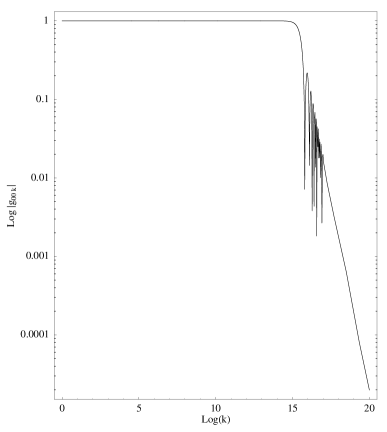
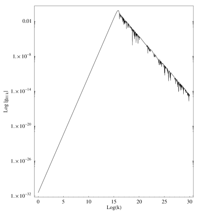
(a)	(b)

Figure 1: The couplings $\log|g_{00k}|$ and $\log|g_{01k}|$ (with $g$ in units of $M_{P}^{-1}$) as functions of $\log k$, for $R=0.2$ mm and $L=1$ TeV^-1. The sharp dips in the curves are bad renderings of a function with narrowly spaced zeros.

Non-diagonal couplings are particularly interesting. Consider $g_{01k}$, the gravitons’ coupling to the fundamental and first-excited scalar branons:

$$g_{01k}=\frac{i\sqrt{2}}{M_{P}}\,\frac{\xi k\left(1-e^{i\frac{k}{\xi}}\right)}{k^{2}-(2\pi\xi)^{2}}~{}.$$ (6)

In Fig. 1(b) we show the “transition form factor” $g_{01k}$ as a function of $k$. For $k\ll\xi$, $g_{01k}$ vanishes as $k^{2}$, the graviton has too little 5-th momentum to undo the orthogonality of $\phi^{0}$ and $\phi^{1}$. For $k={\cal O}(\xi)$ this selection rule is avoided, as the $k$-th graviton can absorb the momentum inbalance. For even larger $k$ the form factor effect takes over and $g_{01k}\!\to\!0$. The explicit expressions in Eqs. (5) and (6) are specific to our toy model of confinement to a brane, but their general behaviour is the one to be intuitively expected: it would be quite similar in any other simple model. The fact that $g_{01k}\!\propto\!k^{2}$ and $g_{00k}\!\propto\!k^{0}$ at low $k$ is general: it can be derived in an “effective field-theory” sense. These non-trivial form factors have interesting consequences, as we shall see.

The fermions of the Standard Model occur in chiral multiplets. It is notoriously difficult to generate these objects in field-theoretic models of dimensional compactification. In heterotic string theories it is customary to face this problem by locating fermions in the singular points of orbifolds (such as $y\!=\!0,\pi$ in a circle $0\!<\!y\!\leq\!2\pi$ subject to the identification $y\leftrightarrow-y$). In generalizations to brane constructs, the role of the orbifold singularities is played by intersections of branes. We abstract from all this the possibility that fermions be confined to spaces more singular than the corresponding ones for bosons, as is often done in the literature without further ado [18]. We shall, in turn, study this possibility and its negation. Reconsider the scalar field attached to a fat brane that we have discussed, $\phi(x,y)$, and its trilinear coupling $\bar{\psi}\psi\phi$ to a fermion that is placed at a specific $y$-location: $\psi(x,y)\propto\psi(x)\delta(y)$. As in the case of graviton’s KK–recurrences, this breakdown of $y$-translational symmetry implies that there are no selection rules in the coupling $\bar{\psi}\psi\phi^{n}$: it does not vanish for branons with $n\neq 0$. This opens up an avenue to a very rich phenomenology, as we proceed to discuss in the specific case of QED on a fat brane.

The minimum number of extra large dimensions of conceivable empirical interest is $\delta=2$. This number is also the most amenable to experimental escrutiny and, in most of what follows, we concentrate on it. Paraphrasing [13], we introduce a 6-vector $Y^{M}$, the first 4 of whose entries are the ordinary coordinates $x$ (with indices $\mu$, $\nu$,…) while the remaining two, labelled $y$ (with indices $a$, $b$,… for $M=5,6$) are the Goldstone fields specifying the position of the 3-brane in the bulk. On the brane, the 6-d metric $G^{MN}$ induces a 4-d metric:

$$g_{\mu\nu}(x,y)=G^{MN}(x,y)~{}\partial_{\mu}Y^{M}(x)~{}\partial_{\nu}Y^{N}(x)\;.$$ (7)

The brane action is akin to the one studied in [13] but for the fact that we use a fat brane with a shape $B(y)$:

$$S=\int d^{4}x\,d^{2}y~{}\sqrt{-g}~{}B(y)~{}[-f^{4}+g_{\mu\nu}(x,y)\;T^{\mu\nu}(x,y)]\,+\,...$$ (8)

where the brane’s tension $f$ induces an energy density profile $f^{4}\,B(y)$. The ellipsis in Eq. (8) stands for higher-order terms in $(\partial Y/f)$ and/or $L/R$, resulting from the extra-dimensional components of the energy–stress tensor. They are associated to phonon emission, and suppressed in comparison with the effects we study.

We begin by discussing the $\delta\!=\!2$ fat-brane scenario with bosons confined to a domain of width $L$. Let $B(y)$, once again, be simply modelled as a square box. Fermions, as we discussed, will first be treated more singularly: $B(y)\to\delta(y)$. The fat-brane QED action (neglecting all terms involving phonons) is then:

$$S_{QED}\!=\!\int\!d^{4}x\,d^{2}y\sqrt{-g}\,B(y)\,g^{\mu\nu}\Big{\{}i\bar{\psi}(x)\gamma_{\mu}D_{\nu}\psi(x)\,\delta(y)+\frac{1}{4}\;F_{\mu M}(x,y){F^{M}}_{\nu}(x,y)\Big{\}}$$ (9)

where $D_{\mu}=\partial_{\mu}-ie_{6}A_{\mu}(x,y)$; and $e_{6}=e\,L$: the 6-d electromagnetic coupling.

We KK-expand $G^{MN}$ as in Eq. (1). We also develop the photon and photoscalars into towers of branons:

$$A_{M}(x,y)=A_{M}^{(\vec{0})}(x)+\sqrt{\frac{2}{L}}\;\sum_{\vec{n}}\cos\left[{\frac{2\pi}{L}\,\vec{n}\cdot\vec{y}}\right]A_{M}^{(\vec{n})}(x)\;\;\;\;\;\;n_{i}\geq 0,$$ (10)

where $\vec{n}=(n_{1},n_{2})$. Half of the 4-d scalar components of the photon $A_{M}$ are gauge artefacts, which the gauge condition $\partial_{M}A^{M}(x,y)=0$ eliminates. The 4-d excited modes of the photon (the branons) acquire mass through a Higgs mechanism that removes from the spectrum all photoscalars other than the zero-modes. All in all, the 6-d fields $A_{M}$ result in a 4-d massless photon, its massive vector excitations and two massless photoscalars (one for each extra dimension).

The branon mass splitting is $m=2\pi/L$. The lower bounds on the masses of excited photons and Z’s are of ${\cal O}$(1 TeV). The next generation of colliders can only hope to see or intuit the lowest excitations, to which we restrict the remaining discussion. Rotate the massive photons, $A_{\mu}^{(\pm)}\!=\!(A_{\mu}^{(1,0)}\pm A_{\mu}^{(0,1)})/\sqrt{2}$, and rescale the zero-mode photoscalars $A_{a}^{(\vec{0})}\to\sqrt{2}A_{a}^{(\vec{0})}$ in Eq. (9), to obtain:

$$S_{QED} \simeq \int d^{4}x\Big{\{}i\bar{\psi}\gamma^{\mu}\partial_{\mu}\psi+e\bar{\psi}\gamma^{\mu}\left[A_{\mu}^{(\vec{0})}+\sqrt{2}A_{\mu}^{(+)}\right]\psi$$ (11)

$$- \sum_{i=\vec{0},+,-}\frac{1}{4}\,F_{\mu\nu}^{(i)}F^{\mu\nu(i)}+\frac{1}{2}\,\partial_{\mu}A_{a}^{(\vec{0})}\partial^{\mu}A_{a}^{(\vec{0})}$$

$$- \frac{1}{4}\,m^{2}\sum_{i=+,-}A_{\mu}^{(i)}A^{\mu(i)}-\frac{1}{M_{P}}\sum_{\vec{k}}H^{\mu\nu(\vec{k})}T_{\mu\nu}^{(\vec{k})}\Big{\}}\,.$$

The gravitational couplings of the zero and first-excited modes can be read from

$$T_{\mu\nu}^{(\vec{k})} = i\bar{\psi}\gamma_{\mu}\partial_{\nu}\psi+e\bar{\psi}\gamma_{\mu}\left(A_{\nu}^{(\vec{0})}+\sqrt{2}A_{\nu}^{(+)}\right)\psi$$ (12)

$$+ \frac{1}{4}\,\,g_{0}^{(k_{1},k_{2})}\left(F_{\mu\rho}^{(\vec{0})}{{F^{\rho}}_{\nu}}^{(\vec{0})}+2\partial_{\mu}A_{a}^{(\vec{0})}\partial_{\nu}A_{a}^{(\vec{0})}\right)$$

$$+ \frac{1}{2\sqrt{2}}\,\,(g_{1}^{(k_{1},k_{2})}\pm g_{1}^{(k_{2},k_{1})})F_{\mu\rho}^{(\vec{0})}{{F^{\rho}}_{\nu}}^{(\pm)}$$

$$- i\sqrt{2}\;m\left(g_{1}^{(k_{1},k_{2})}\partial_{\mu}A_{1}^{(\vec{0})}\pm g_{1}^{(k_{2},k_{1})}\partial_{\mu}A_{2}^{(\vec{0})}\right)A_{\nu}^{(\pm)}\,,$$

where we have defined $g_{i}^{(k_{1},k_{2})}\!=\!M_{P}\,g_{0ik_{1}}\,g_{00k_{2}}$, to extend the $\delta\!=\!1$ results of Eqs. (5) and (6) to one more extra dimension.

Following the weird but deeply rooted habit of denoting many fields differently from their corresponding quanta, let $G^{(\vec{k})}$ be the gravitons of the field $H^{(\vec{k})}$, $\gamma$ and $\gamma^{*}$ be the photons of the fields $A_{\mu}^{(\vec{0})}$ and $A_{\mu}^{(+)}$, and $\tilde{\gamma}_{a}$, with $a\,=\,1,2$, the photoscalars of the fields $A_{a}^{(\vec{0})}$. Fermions, as in Eq. (11), couple to $\gamma$ and $\gamma^{*}$, but not to the odd massive vector mode, which will play no role here, nor to the massless photoscalars $\tilde{\gamma}$, for which a minor role is reserved. The $\gamma\gamma G^{(\vec{k})}$ vertex in Eq. (12), relative to its standard gravitational strength in the thin-brane limit [16, 17], is reduced for a fat brane by a form factor $g_{0}^{(k_{1},k_{2})}$. More interestingly, a new coupling $\gamma^{*}\gamma\,G^{(\vec{k})}$ appears, allowing the excited photons $\gamma^{*}$ to decay into gravitons and an ordinary photon. This non-diagonal coupling is modulated by the “transition form factor” $g_{1}^{(k_{1},k_{2})}+g_{1}^{(k_{2},k_{1})}$. The coupling of $\gamma^{*}$ to fermions, which is so interesting in view of the possibility of producing such a resonance in $e^{+}e^{-}$ or $\mu^{+}\mu^{-}$ collisions, arises only if the fermions are located differently from the photons in the extra dimensions (this is the usual assumption [18], adopted in our fat-brane scenario). In an alternative scenario, in which the fermions are also spread over the width $L$ of the brane, as the bosons described in Eq. (10) are, the $e^{+}e^{-}\gamma^{*}$ coupling is forbidden by a KK momentum-conservation selection rule. For such boson–fermion symmetric superfat branes, the $\bar{\psi}\gamma^{\mu}\psi A_{\mu}^{+}$ coupling in Eq. (11) should be removed.

Armed with the action of Eqs. (11) and (12), one can proceed to compute a phenomenologically interesting process, such as the production, in an $e^{+}e^{-}$ or $\mu^{+}\mu^{-}$ collider, of single photons plus (invisible) gravitons: $\ell^{+}\ell^{-}\to\gamma+E_{\rm mis}$. For the fat brane this process will be dominated by the $\gamma^{*}$ s-channel resonance. To facilitate the comparison with previous work on thin branes by Giudice et al. [16], which we have checked to be correct, we shall concentrate on a hypothetical $\sqrt{s}=1$ TeV collider, and present cross sections with the same cuts as they use (a transverse energy cut $E_{T,\gamma}\equiv p_{\gamma}\,\sin\theta$ $\geq E_{T,\gamma}^{\rm min}$ to avoid collinear divergences and a cut $E_{\gamma}\leq$ 450 GeV to avoid the dominant $\gamma\,Z\to\gamma\nu\bar{\nu}$ background). In a letter we cannot present a plethora of results and we mainly discuss the $\delta\!=\!2$ case, even if it is presumably marginalized, for parameters in the range we shall study, by astrophysical considerations [19]. Our main message –on how rich the phenomenology can be– is sufficiently illustrated by this case, though for the most interesting observables we also work out results for $\delta=4,\,6$. The parameters to be varied are the “new-physics” scale $M$ and the width of the brane $L$ or, equivalently, the mass of the $\gamma^{*}$, $m=2\pi/L$. We do not know the exact relation between $m$ and $M$, which should be of the same order of magnitude ($R$ is related to $M$ by $M_{P}^{2}\!=\![2\pi R]^{\delta}M^{\delta+2}$).

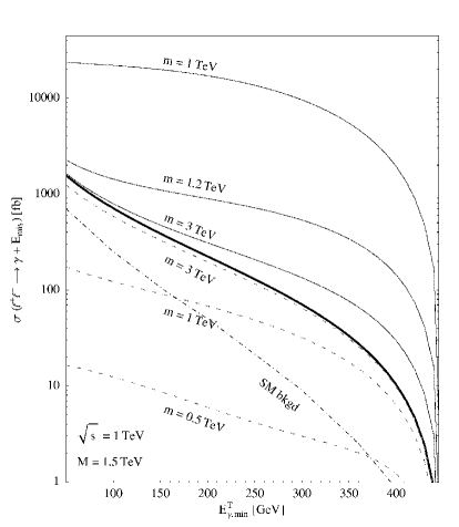
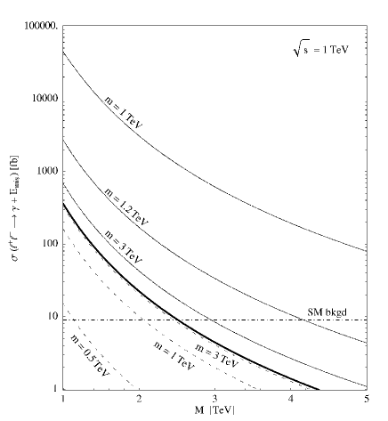
(a)	(b)

Figure 2: The cross sections for $\ell^{+}\ell^{-}\to\gamma+E_{\rm mis}$ at $\sqrt{s}=1$ TeV, for $\delta\!=\!2$. (a) As a function of $E_{T,\gamma}^{\rm min}$. (b) Integrated for $E_{T,\gamma}\!>\!300$ GeV. The thick line in a) and b) is for thin branes. Curves above (below) it are for fat (superfat) branes.

From the point of view of experimental observability, fat and superfat branes turn out to be, respectively, the optimistic and pessimistic extremes, while thin branes are in between. This can be seen in Fig. 2, where we present results for a lepton collider running at $\sqrt{s}=1$ TeV. In Fig. 2(a) we show the cross section for $\ell^{+}\ell^{-}\to\gamma+E_{\rm mis}$, integrated for $E_{T,\gamma}\geq E_{T,\gamma}^{\rm min}$ for various values of $m$ and a fixed $M=1.5$ TeV. The results scale as $M^{-4}$, as can be explicitly seen in Fig. 2(b) for the total cross section (within cuts) as a function of $M$. In both of these figures the thick continuous line is the thin-brane limit [16]. The continuous curves are fat-brane results, they peak for $m=1$ TeV, when our assumed collider is running at the $\gamma^{*}$ resonant peak. The dashed curves are for superfat branes (in the labels of these curves $m$ is a shorthand for $2\pi/L$, the $\gamma^{*}$ exists, but is not an $\ell^{+}\ell^{-}$ resonance in this case). The dash-dotted line is the Standard Model background, as estimated in [16]. The signal over background ratios are very favourable, except for superfat branes at small $m$, for which the form-factor effects quench the signal very significantly.

In any model with branons, KK recurrences, or any other sequential gauge bosons that couple to fermions, the $\ell^{+}\ell^{-}$ total annihilation cross section would have the obvious resonant-peak signatures, no doubt interestingly intertwined [18, 20], since a $Z^{*}$ peak at $s=m^{2}+M_{Z}^{2}$ is to be expected, with $m$ the mass of $\gamma^{*}$. The total cross section, however, would not distinguish the objects we are discussing –related to bulk dimensions in which only gravitons dwell– from more conventional KK excitations. We thus concentrate on a specific final state: $\gamma$ plus unobserved gravitons. In Fig. 3 we show $\sigma(\ell^{+}\ell^{-}\to\gamma+E_{\rm mis})$ as a function of $\sqrt{s}$ for the case of fat branes, for $m=1,\,1.5,\,2$ TeV and $M=1,\,5$ TeV, all for $\delta=2$. Also shown, for comparison, is the thin-brane result [16].

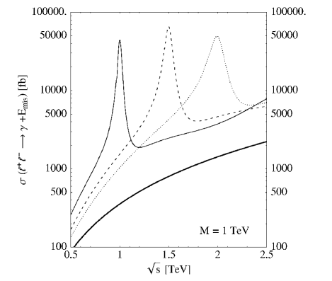
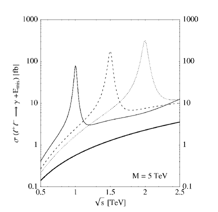
(a)	(b)

Figure 3: The fat-brane resonant cross sections for $\ell^{+}\ell^{-}\to\gamma+E_{\rm mis}$ as a function of $\sqrt{s}$, for $M=1$ TeV (a) and $M=5$ TeV (b), for $\delta=2$. The non-resonant curves are thin-brane results.

The fat-brane results of Figs. 2 and 3 depend on the total and partial widths of the $\gamma^{*}$ resonance, which we now discuss in some detail. At tree level, $\gamma^{*}$ decays into charged lepton pairs , hadrons ($q\bar{q}$ pairs), photon plus gravitons ($\gamma\,G^{(\vec{k})}$) and scalar photon plus gravitons ($\tilde{\gamma}\,G^{(\vec{k})}$), an “invisible” decay channel. The widths into all these channels can be worked out from the action of Eqs. (11) and (12), and its generalization to fractionally charged quarks. For the fermion channels we obtain $\Gamma_{\gamma^{*}}(q\bar{q})\simeq 1.6\times 10^{-2}\;m$ and $\Gamma_{\gamma^{*}}(\ell^{+}\ell^{-})\simeq 2.6\times 10^{-2}\;m$, independent of $M$ and $\delta$.

For the $\gamma^{*}\!\to\!\gamma\,G^{(\vec{k})}$ decays, a fixed photon energy $E_{\gamma}$ corresponds to a given graviton mass $|\vec{k}|/R$ in their quasi-continuum mass distribution. Define $x\!\equiv\!2\,E_{\gamma}/m$, so that $x=1-|\vec{k}|^{2}/(mR)^{2}$ and $0\!\leq\!x\!\leq\!1$. The differential width is of the form:

$${d\,\Gamma_{\delta}\over dx}=m\;\left({m\over M}\right)^{\delta+2}\;{d\,\chi_{\delta}\over dx}\;,$$ (13)

where the scaled width $d\chi_{\delta}/dx$ is independent of $M$ and $m$. For the case $\delta\!=\!2$, define $\alpha\!\equiv\!\arctan(k_{1}/k_{2})$ and let $g(x,\alpha)$ be a shorthand for $g_{1}^{(k_{1},k_{2})}+g_{1}^{(k_{2},k_{1})}$. For the scaled width in Eq. (13), we get:

$${d\chi_{2}\over dx}={M_{P}^{2}\,x\over 96\,\pi}\;\int_{0}^{2\pi}\,d\alpha\;\left\{{|g|^{2}\over 12}\;{x^{2}\over(1-x)^{2}}\;\left[10-15x+6x^{2}\right]\right\}\;,$$ (14)

where the quantity in wiggly brackets is the square of the transition matrix element for $\gamma^{*}\!\to\!\gamma\,G^{(\vec{k})}$ decay and depends, via $g$, on the form factors specific to a particular model of confinement to a brane. In our model, for the total ($x$-integrated) width $\gamma^{*}\rightarrow\gamma\,G$, we obtain $\chi_{2}=1.1\times 10^{-3}$, to be substituted in Eq. (13). The $\gamma^{*}\rightarrow\tilde{\gamma}\,G$ width has the same dependence on $m$ and $M$, with a different coefficient, $\tilde{\chi}_{\delta}$. For $\delta=2$, $\tilde{\chi}_{2}=5.7\times 10^{-4}$. The generalization of Eq. (14) to $\delta\!>\!2$ is rather straightforward [14]. The integrated widths for $\gamma^{*}\!\to\!\gamma\,G$ are given by Eq. (13), with $\chi_{4}=1.0$ and $\chi_{6}=7.4\times 10^{2}$. The rapid growth of $\chi_{\delta}$ with $\delta$ reflects how fast the number of accessible KK excitations increases, as new dimensions are added.

In Fig. 4(a) we show the total and partial widths of the $\gamma^{*}$ as functions of $m$, for $M\!=\!1,\,5$ TeV and $\delta\!=\!2$. For the smaller and most accessible $\gamma^{*}$ masses the partial width into fermions dominates. But even at these relatively small $m$, for $M$ also of ${\cal O}(1)$ TeV, the $\gamma^{*}\to\gamma\,G$ branching ratio is large enough to constitute a striking signal. Only for $M$ large relative to $m$ do the branching ratios into this tell-tale channel become unfavourably small. For $\delta>2$ the resonances get wider: they remain prominent peaks only for sufficiently small $m/M$, as dictated by Eq. (13).

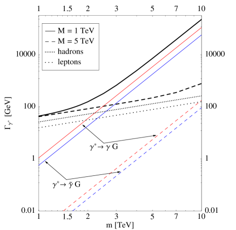
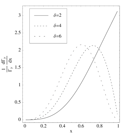
(a)	(b)

Figure 4: (a) Partial and total widths of the $\gamma^{*}$ resonance, as functions of its mass, $m$, for $\delta=2$. The continuous (dashed) curves are for $M=1,\,5$ TeV. The dotted lines are partial widths into quarks and leptons. (b) The decay spectrum $d\Gamma_{\gamma}/(\Gamma_{\gamma}\,dx)$ for $\gamma^{*}\to\gamma+E_{\rm mis}$ as a function of $x$, for three values of $\delta$.

In Fig. 4(b) we show the most spectacular fat-brane signal: the spectrum of photon energies in $\gamma^{*}\!\to\!\gamma\,G$ decay. This distribution is a superposition of the peaks associated with the individual gravitons of different mass, but their number is so huge as to make their resolution impossible. The scaled function $d\Gamma_{\gamma}/(\Gamma_{\gamma}\,dx)$ is independent of $M$ and $m$; it only depends on $\delta$ and on the explicit branon wave functions, of which Eq. (10) is an example. Only the $\delta$-dependence survives as $x$ approaches unity, since this region corresponds to decays into the lighter gravitons, for which the power behaviour of the form factors of Eqs. (5) and (6) and Fig. 1 is model-independent: the matrix element in Eq. (14) and its generalizations to $\delta\!>\!2$ is a polynomial [14] in $x$ ($|g|\!\propto\!(1\!-\!x)^{2}$ as $x\!\to\!1$). Close to $x=1$ we obtain:

$$\frac{1}{\Gamma_{\gamma}}\frac{d\Gamma_{\gamma}}{dx}\propto(1-x)^{(\delta-2)/2}\;\left[1+{\cal O}\left([1-x]\right)\right]$$ (15)

A two-body decay into a $\gamma$ and a single invisible particle would result in a peak with a width governed by resolution, looking nothing like the curves of Fig. 4(b). A three-body decay involving two invisible particles –with form factors contrived to imitate one of the shapes in the figure– is the only implausible impostor. Thus, the measurement of $d\Gamma_{\gamma}/(\Gamma_{\gamma}\,dx_{\gamma})$ would be a convincing signal for the existence of extra dimensions, and its behaviour as $x$ approaches its upper limit would constitute a very neat dimensiometer.

To summarize, the message conveyed by Figs. 2–4 is clear: the physics at energies at which new dimensions “open up” can range from the very challenging to the very rich. The phenomenological signals so far studied in the literature [16, 17] can be wiped-out by “form-factor” effects if branes are “superfat” and have widths of the natural order of magnitude. On the other hand, if chiral fermions are special and localized in slices of space-time thinner than those in which bosons reside –as for the more standard fat branes– the production of KK-like “branon” resonances in collisions between ordinary particles becomes possible. The decays of excited $\gamma$’s or $Z$’s into their ground states plus unobservable gravitons would provide astounding signals. In particular, the energy distribution of the final-state $\gamma$ or $Z$ would not be sharply peaked (as for a conventional two-body decay), its spread reflecting the mass distribution of the accompanying tower of gravitons, and its high-energy tail providing a direct measurement of $\delta$, the number of large extra dimensions.

At high energy, ideas about large extra dimensions will first confront new data at the LHC $pp$ collider, as we plan to discuss in subsequent work. In the fat-brane scenario, the $q\bar{q}$ production of $Z^{*}$ –the first branon excitation of the $Z$– and its decay into $Z$ plus KK gravitons, constitute the most spectacular signatures. The energy distribution of the observed $Z$’s, because of the unobservable longitudinal momentum of the colliding partons, is not as gorgeous a signal as its lepton-collider counterpart. But this inconvenience is compensated by large statistics and, what’s more, by the LHC’s appropinquity.

References

-
[1]
T. Kaluza,
Sitzungsberichte of the Prussian Acad. of Sci. (1921) 966;
O. Klein, Z. Phys. 37 (1926) 895. - [2] V. Rubakov and M. Shaposhnikov, Phys. Lett. B 125 (1983) 136.
- [3] P. Horava and E. Witten, Nucl. Phys. B 460 (1996) 506; Nucl. Phys. B475 (1996) 94.
- [4] I. Antoniadis, Phys. Lett. B246 (1990) 377.
- [5] N. Arkani-Hamed, S. Dimopoulos and G. Dvali, Phys. Lett. B 429 (1998) 263; I. Antoniadis, N. Arkani-Hamed, S. Dimopoulos and G. Dvali, Phys. Lett. B 436 (1998) 257;
- [6] J. D. Lykken, Phys. Rev. D54 (1996) 3693.
- [7] For a recent review see for example T. Banks, M. Dine and A. Nelson, JHEP 9906 (1999) 014 and reference therein.
- [8] J. Polchinski, hep-th/9611050.
- [9] G. Aldazabal, A. Font, L. E. Ibáñez and G. Violero, Nucl. Phys. B536 (1998) 29; L. E. Ibáñez, C. Muñoz and S. Rigolin, Nucl. Phys. B553 (1999) 43; G. Aldazabal, L. E. Ibáñez and F. Quevedo, JHEP 0001 (2000) 31 and hep-ph/0001083.
- [10] K. R. Dienes, E. Dudas and T. Gherghetta, Nucl. Phys. B537 (1999) 47.
- [11] N. Arkani-Hamed and M. Schmaltz, Phys. Rev. D61 (2000) 033005; N. Arkani-Hamed, Y. Grossman and M. Schmaltz, hep-ph/9909411.
- [12] This point has also been investigated, though very differently, in M. Bando, T. Kugo, T. Noguchi and K. Yoshioka, Phys. Rev. Lett. 83 (1999) 3601; J. Hisano and N. Okada, hep-ph/9909555; T. Kugo and K. Yoshioka, hep-ph/9912496.
- [13] R. Sundrum, Phys. Rev. D 59 (1999) 085009.
- [14] A detailed discussion will appear in a paper in preparation by the present authors.
- [15] N. Arkani-Hamed, S. Dimopoulos and G. Dvali, Phys. Rev. D 59 (1999) 086004.
- [16] G. Giudice, R. Rattazzi and J. Wells, Nucl. Phys. B 544 (1999) 3.
-
[17]
E. A. Mirabelli, M. Perelstein and M. E. Peskin,
Phys. Rev. Lett. 82 (1999) 2236;
T. Han, J. D. Lykken and R.-J. Zhang, Phys. Rev. D 59 (1999) 105006. - [18] I. Antoniadis, C. Muñoz and M. Quirós, Nucl. Phys. B397 (1993) 515; I. Antoniadis, K. Benakli and M. Quirós, Phys. Lett. B331 (1994) 313, and references therein.
- [19] S. Cullen and M. Perelstein, Phys. Rev. Lett. 83 (1999) 268. For cosmological limits, see L. J. Hall and D. Smith, Phys. Rev. D60 (1999) 085008.
- [20] A. Donini and S. Rigolin, Nucl. Phys. B550 (1999) 59 and hep-ph/9905293; I. Antoniadis, K. Benakli and M. Quirós, Phys. Lett. B460 (1999) 176; E. Accomando, I. Antoniadis and K. Benakli, hep-ph/9912287.
- [21] E. Dudas and J. Mourad, hep-th/9911019.
- [22] S. Cullen, M. Perelstein and M. E. Peskin, hep-ph/0001166.