INTRODUCTION TO B PHYSICS

These lectures provide an introduction to various topics in heavy-flavor physics. We review the theory and phenomenology of heavy-quark symmetry, exclusive weak decays of $B$ mesons, inclusive decay rates, and some rare $B$ decays.

1 Introduction

The rich phenomenology of weak decays has always been a source of information about the nature of elementary particle interactions. A long time ago, $\beta$- and $\mu$-decay experiments revealed the structure of the effective flavor-changing interactions at low momentum transfer. Today, weak decays of hadrons containing heavy quarks are employed for tests of the Standard Model and measurements of its parameters. In particular, they offer the most direct way to determine the weak mixing angles, to test the unitarity of the Cabibbo-Kobayashi-Maskawa (CKM) matrix, and to explore the physics of CP violation. Hopefully, this will provide some hints about New Physics beyond the Standard Model. On the other hand, hadronic weak decays also serve as a probe of that part of strong-interaction phenomenology which is least understood: the confinement of quarks and gluons inside hadrons.

The structure of weak interactions in the Standard Model is rather simple. Flavor-changing decays are mediated by the coupling of the charged current $J_{\rm CC}^{\mu}$ to the $W$-boson field:

$${\cal L}_{\rm CC}=-{g\over\sqrt{2}}\,J_{\rm CC}^{\mu}\,W_{\mu}^{\dagger}+\mbox{h.c.,}$$ (1)

where

$$J_{\rm CC}^{\mu}=(\bar{\nu}_{e},\bar{\nu}_{\mu},\bar{\nu}_{\tau})\,\gamma^{\mu}\left(\begin{array}[]{c}e_{\rm L}\\ \mu_{\rm L}\\ \tau_{\rm L}\end{array}\right)+(\bar{u}_{\rm L},\bar{c}_{\rm L},\bar{t}_{\rm L})\,\gamma^{\mu}\,V_{\rm CKM}\left(\begin{array}[]{c}d_{\rm L}\\ s_{\rm L}\\ b_{\rm L}\end{array}\right)$$ (2)

contains the left-handed lepton and quark fields, and

$$V_{\rm CKM}=\left(\begin{array}[]{ccc}V_{ud}&V_{us}&V_{ub}\\ V_{cd}&V_{cs}&V_{cb}\\ V_{td}&V_{ts}&V_{tb}\end{array}\right)$$ (3)

is the CKM matrix. At low energies, the charged-current interaction gives rise to local four-fermion couplings of the form

$${\cal L}_{\rm eff}=-2\sqrt{2}G_{F}\,J_{\rm CC}^{\mu}J_{{\rm CC},\mu}^{\dagger}\,,$$ (4)

where

$$G_{F}={g^{2}\over 4\sqrt{2}M_{W}^{2}}=1.16639(2)~{}\mbox{GeV}^{-2}$$ (5)

is the Fermi constant.

Figure 1: Examples of leptonic ($B^{-}\to\tau^{-}\bar{\nu}_{\tau}$), semi-leptonic ($\bar{B}^{0}\to D^{+}e^{-}\bar{\nu}_{e}$), and non-leptonic ($\bar{B}^{0}\to D^{+}\pi^{-}$) decays of $B$ mesons.

According to the structure of the charged-current interaction, weak decays of hadrons can be divided into three classes: leptonic decays, in which the quarks of the decaying hadron annihilate each other and only leptons appear in the final state; semi-leptonic decays, in which both leptons and hadrons appear in the final state; and non-leptonic decays, in which the final state consists of hadrons only. Representative examples of these three types of decays are shown in Fig. 1. The simple quark-line graphs shown in this figure are a gross oversimplification, however. In the real world, quarks are confined inside hadrons, bound by the exchange of soft gluons. The simplicity of the weak interactions is overshadowed by the complexity of the strong interactions. A complicated interplay between the weak and strong forces characterizes the phenomenology of hadronic weak decays. As an example, a more realistic picture of a non-leptonic decay is shown in Fig. 2.

Figure 2: More realistic representation of a non-leptonic decay.

The complexity of strong-interaction effects increases with the number of quarks appearing in the final state. Bound-state effects in leptonic decays can be lumped into a single parameter (a “decay constant”), while those in semi-leptonic decays are described by invariant form factors depending on the momentum transfer $q^{2}$ between the hadrons. Approximate symmetries of the strong interactions help us to constrain the properties of these form factors. Non-leptonic weak decays, on the other hand, are much more complicated to deal with theoretically. Only very recently reliable tools have been developed that allow us to control the complex QCD dynamics in many two-body $B$ decays using a heavy-quark expansion.

Over the last decade, a lot of information on heavy-quark decays has been collected in experiments at $e^{+}e^{-}$ storage rings operating at the $\Upsilon(4s)$ resonance, and more recently at high-energy $e^{+}e^{-}$ and hadron colliders. This has led to a rather detailed knowledge of the flavor sector of the Standard Model and many of the parameters associated with it. In the years ahead the $B$ factories at SLAC, KEK, Cornell, and DESY will continue to provide a wealth of new results, focusing primarily on studies of CP violation and rare decays.

The experimental progress in heavy-flavor physics has been accompanied by a significant progress in theory, which was related to the discovery of heavy-quark symmetry, the development of the heavy-quark effective theory, and more generally the establishment of various kinds of heavy-quark expansions. The excitement about these developments rests upon the fact that they allow model-independent predictions in an area in which “progress” in theory often meant nothing more than the construction of a new model, which could be used to estimate some strong-interaction hadronic matrix elements. In Sec. 2, we review the physical picture behind heavy-quark symmetry and discuss the construction, as well as simple applications, of the heavy-quark effective theory. Section 3 deals with applications of these concepts to exclusive weak decays of $B$ mesons. Applications of the heavy-quark expansion to inclusive $B$ decays are reviewed in Sec. 4. We then focus on the exciting field of rare hadronic $B$ decays, concentrating on the example of the decays $B\to\pi K$. In Sec. 5, we discuss the theoretical description of these decays and explain various strategies for constraining and determining the weak, CP-violating phase $\gamma=\mbox{arg}(V_{ub}^{*})$ of the CKM matrix. In Sec. 6, we discuss how rare decays can be used to search for New Physics beyond the Standard Model.

2 Heavy-Quark Symmetry

This section provides an introduction to the ideas of heavy-quark symmetry $\!{}^{{\bf?}}$^-$\!{}^{{\bf?}}$ and the heavy-quark effective theory $\!{}^{{\bf?}}$^-$\!{}^{{\bf?}}$, which provide the modern theoretical framework for the description of the properties and decays of hadrons containing a heavy quark. For a more detailed description of this subject, the reader is referred to the review articles in Refs. 18–24.

2.1 The Physical Picture

There are several reasons why the strong interactions of hadrons containing heavy quarks are easier to understand than those of hadrons containing only light quarks. The first is asymptotic freedom, the fact that the effective coupling constant of QCD becomes weak in processes with a large momentum transfer, corresponding to interactions at short distance scales $\!{}^{{\bf?},{\bf?}}$. At large distances, on the other hand, the coupling becomes strong, leading to non-perturbative phenomena such as the confinement of quarks and gluons on a length scale $R_{\rm had}\sim 1/\Lambda_{\rm QCD}\sim 1$ fm, which determines the size of hadrons. Roughly speaking, $\Lambda_{\rm QCD}\sim 0.2$ GeV is the energy scale that separates the regions of large and small coupling constant. When the mass of a quark $Q$ is much larger than this scale, $m_{Q}\gg\Lambda_{\rm QCD}$, it is called a heavy quark. The quarks of the Standard Model fall naturally into two classes: up, down and strange are light quarks, whereas charm, bottom and top are heavy quarks. For heavy quarks, the effective coupling constant $\alpha_{s}(m_{Q})$ is small, implying that on length scales comparable to the Compton wavelength $\lambda_{Q}\sim 1/m_{Q}$ the strong interactions are perturbative and much like the electromagnetic interactions. In fact, the quarkonium systems $(\bar{Q}Q)$, whose size is of order $\lambda_{Q}/\alpha_{s}(m_{Q})\ll R_{\rm had}$, are very much hydrogen-like.

Systems composed of a heavy quark and other light constituents are more complicated. The size of such systems is determined by $R_{\rm had}$, and the typical momenta exchanged between the heavy and light constituents are of order $\Lambda_{\rm QCD}$. The heavy quark is surrounded by a complicated, strongly interacting cloud of light quarks, antiquarks and gluons. In this case it is the fact that $\lambda_{Q}\ll R_{\rm had}$, i.e. that the Compton wavelength of the heavy quark is much smaller than the size of the hadron, which leads to simplifications. To resolve the quantum numbers of the heavy quark would require a hard probe; the soft gluons exchanged between the heavy quark and the light constituents can only resolve distances much larger than $\lambda_{Q}$. Therefore, the light degrees of freedom are blind to the flavor (mass) and spin orientation of the heavy quark. They experience only its color field, which extends over large distances because of confinement. In the rest frame of the heavy quark, it is in fact only the electric color field that is important; relativistic effects such as color magnetism vanish as $m_{Q}\to\infty$. Since the heavy-quark spin participates in interactions only through such relativistic effects, it decouples.

It follows that, in the limit $m_{Q}\to\infty$, hadronic systems which differ only in the flavor or spin quantum numbers of the heavy quark have the same configuration of their light degrees of freedom $\!{}^{{\bf?}}$^-$\!{}^{{\bf?}}$. Although this observation still does not allow us to calculate what this configuration is, it provides relations between the properties of such particles as the heavy mesons $B$, $D$, $B^{*}$ and $D^{*}$, or the heavy baryons $\Lambda_{b}$ and $\Lambda_{c}$ (to the extent that corrections to the infinite quark-mass limit are small in these systems). These relations result from some approximate symmetries of the effective strong interactions of heavy quarks at low energies. The configuration of light degrees of freedom in a hadron containing a single heavy quark with velocity $v$ does not change if this quark is replaced by another heavy quark with different flavor or spin, but with the same velocity. Both heavy quarks lead to the same static color field. For $N_{h}$ heavy-quark flavors, there is thus an SU$(2N_{h})$ spin-flavor symmetry group, under which the effective strong interactions are invariant. These symmetries are in close correspondence to familiar properties of atoms. The flavor symmetry is analogous to the fact that different isotopes have the same chemistry, since to good approximation the wave function of the electrons is independent of the mass of the nucleus. The electrons only see the total nuclear charge. The spin symmetry is analogous to the fact that the hyperfine levels in atoms are nearly degenerate. The nuclear spin decouples in the limit $m_{e}/m_{N}\to 0$.

Heavy-quark symmetry is an approximate symmetry, and corrections arise since the quark masses are not infinite. In many respects, it is complementary to chiral symmetry, which arises in the opposite limit of small quark masses. There is an important distinction, however. Whereas chiral symmetry is a symmetry of the QCD Lagrangian in the limit of vanishing quark masses, heavy-quark symmetry is not a symmetry of the Lagrangian (not even an approximate one), but rather a symmetry of an effective theory that is a good approximation to QCD in a certain kinematic region. It is realized only in systems in which a heavy quark interacts predominantly by the exchange of soft gluons. In such systems the heavy quark is almost on-shell; its momentum fluctuates around the mass shell by an amount of order $\Lambda_{\rm QCD}$. The corresponding fluctuations in the velocity of the heavy quark vanish as $\Lambda_{\rm QCD}/m_{Q}\to 0$. The velocity becomes a conserved quantity and is no longer a dynamical degree of freedom $\!{}^{{\bf?}}$. Nevertheless, results derived on the basis of heavy-quark symmetry are model-independent consequences of QCD in a well-defined limit. The symmetry-breaking corrections can be studied in a systematic way. To this end, it is however necessary to cast the QCD Lagrangian for a heavy quark,

$${\cal L}_{Q}=\bar{Q}\,(i\hbox to0.0pt{\,/\hss}D-m_{Q})\,Q\,,$$ (6)

into a form suitable for taking the limit $m_{Q}\to\infty$.

2.2 Heavy-Quark Effective Theory

The effects of a very heavy particle often become irrelevant at low energies. It is then useful to construct a low-energy effective theory, in which this heavy particle no longer appears. Eventually, this effective theory will be easier to deal with than the full theory. A familiar example is Fermi’s theory of the weak interactions. For the description of the weak decays of hadrons, the weak interactions can be approximated by point-like four-fermion couplings, governed by a dimensionful coupling constant $G_{F}$ [cf. (4)]. The effects of the intermediate $W$ bosons can only be resolved at energies much larger than the hadron masses.

The process of removing the degrees of freedom of a heavy particle involves the following steps $\!{}^{{\bf?}}$^-$\!{}^{{\bf?}}$: one first identifies the heavy-particle fields and “integrates them out” in the generating functional of the Green functions of the theory. This is possible since at low energies the heavy particle does not appear as an external state. However, whereas the action of the full theory is usually a local one, what results after this first step is a non-local effective action. The non-locality is related to the fact that in the full theory the heavy particle with mass $M$ can appear in virtual processes and propagate over a short but finite distance $\Delta x\sim 1/M$. Thus, a second step is required to obtain a local effective Lagrangian: the non-local effective action is rewritten as an infinite series of local terms in an Operator Product Expansion (OPE) $\!{}^{{\bf?},{\bf?}}$. Roughly speaking, this corresponds to an expansion in powers of $1/M$. It is in this step that the short- and long-distance physics is disentangled. The long-distance physics corresponds to interactions at low energies and is the same in the full and the effective theory. But short-distance effects arising from quantum corrections involving large virtual momenta (of order $M$) are not described correctly in the effective theory once the heavy particle has been integrated out. In a third step, they have to be added in a perturbative way using renormalization-group techniques. These short-distance effects lead to a renormalization of the coefficients of the local operators in the effective Lagrangian. An example is the effective Lagrangian for non-leptonic weak decays, in which radiative corrections from hard gluons with virtual momenta in the range between $m_{W}$ and some low renormalization scale $\mu$ give rise to Wilson coefficients, which renormalize the local four-fermion interactions $\!{}^{{\bf?}}$^-$\!{}^{{\bf?}}$.

The heavy-quark effective theory (HQET) is constructed to provide a simplified description of processes where a heavy quark interacts with light degrees of freedom predominantly by the exchange of soft gluons $\!{}^{{\bf?}}$^-$\!{}^{{\bf?}}$. Clearly, $m_{Q}$ is the high-energy scale in this case, and $\Lambda_{\rm QCD}$ is the scale of the hadronic physics we are interested in. The situation is illustrated in Fig. 3. At short distances, i.e. for energy scales larger than the heavy-quark mass, the physics is perturbative and described by conventional QCD. For mass scales much below the heavy-quark mass, the physics is complicated and non-perturbative because of confinement. Our goal is to obtain a simplified description in this region using an effective field theory. To separate short- and long-distance effects, we introduce a separation scale $\mu$ such that $\Lambda_{\rm QCD}\ll\mu\ll m_{Q}$. The HQET will be constructed in such a way that it is equivalent to QCD in the long-distance region, i.e. for scales below $\mu$. In the short-distance region, the effective theory is incomplete, since some high-momentum modes have been integrated out from the full theory. The fact that the physics must be independent of the arbitrary scale $\mu$ allows us to derive renormalization-group equations, which can be employed to deal with the short-distance effects in an efficient way.

Figure 3: Philosophy of the heavy-quark effective theory.

Compared with most effective theories, in which the degrees of freedom of a heavy particle are removed completely from the low-energy theory, the HQET is special in that its purpose is to describe the properties and decays of hadrons which do contain a heavy quark. Hence, it is not possible to remove the heavy quark completely from the effective theory. What is possible is to integrate out the “small components” in the full heavy-quark spinor, which describe the fluctuations around the mass shell.

The starting point in the construction of the HQET is the observation that a heavy quark bound inside a hadron moves more or less with the hadron’s velocity $v$ and is almost on-shell. Its momentum can be written as

$$p_{Q}^{\mu}=m_{Q}v^{\mu}+k^{\mu}\,,$$ (7)

where the components of the so-called residual momentum $k$ are much smaller than $m_{Q}$. Note that $v$ is a four-velocity, so that $v^{2}=1$. Interactions of the heavy quark with light degrees of freedom change the residual momentum by an amount of order $\Delta k\sim\Lambda_{\rm QCD}$, but the corresponding changes in the heavy-quark velocity vanish as $\Lambda_{\rm QCD}/m_{Q}\to 0$. In this situation, it is appropriate to introduce large- and small-component fields, $h_{v}$ and $H_{v}$, by

$$h_{v}(x)=e^{im_{Q}v\cdot x}\,P_{+}\,Q(x)\,,\qquad H_{v}(x)=e^{im_{Q}v\cdot x}\,P_{-}\,Q(x)\,,$$ (8)

where $P_{+}$ and $P_{-}$ are projection operators defined as

$$P_{\pm}={1\pm\hbox to0.0pt{/\hss}v\over 2}\,.$$ (9)

It follows that

$$Q(x)=e^{-im_{Q}v\cdot x}\,[h_{v}(x)+H_{v}(x)]\,.$$ (10)

Because of the projection operators, the new fields satisfy $\hbox to0.0pt{/\hss}v\,h_{v}=h_{v}$ and $\hbox to0.0pt{/\hss}v\,H_{v}=-H_{v}$. In the rest frame, i.e. for $v^{\mu}=(1,0,0,0)$, $h_{v}$ corresponds to the upper two components of $Q$, while $H_{v}$ corresponds to the lower ones. Whereas $h_{v}$ annihilates a heavy quark with velocity $v$, $H_{v}$ creates a heavy antiquark with velocity $v$.

In terms of the new fields, the QCD Lagrangian (6) for a heavy quark takes the form

$${\cal L}_{Q}=\bar{h}_{v}\,iv\!\cdot\!D\,h_{v}-\bar{H}_{v}\,(iv\!\cdot\!D+2m_{Q})\,H_{v}+\bar{h}_{v}\,i\hbox to0.0pt{\,/\hss}D_{\perp}H_{v}+\bar{H}_{v}\,i\hbox to0.0pt{\,/\hss}D_{\perp}h_{v}\,,$$ (11)

where $D_{\perp}^{\mu}=D^{\mu}-v^{\mu}\,v\cdot D$ is orthogonal to the heavy-quark velocity: $v\cdot D_{\perp}=0$. In the rest frame, $D_{\perp}^{\mu}=(0,\vec{D}\,)$ contains the spatial components of the covariant derivative. From (11), it is apparent that $h_{v}$ describes massless degrees of freedom, whereas $H_{v}$ corresponds to fluctuations with twice the heavy-quark mass. These are the heavy degrees of freedom that will be eliminated in the construction of the effective theory. The fields are mixed by the presence of the third and fourth terms, which describe pair creation or annihilation of heavy quarks and antiquarks. As shown in the first diagram in Fig. 4, in a virtual process, a heavy quark propagating forward in time can turn into an antiquark propagating backward in time, and then turn back into a quark. The energy of the intermediate quantum state $hh\bar{H}$ is larger than the energy of the incoming heavy quark by at least $2m_{Q}$. Because of this large energy gap, the virtual quantum fluctuation can only propagate over a short distance $\Delta x\sim 1/m_{Q}$. On hadronic scales set by $R_{\rm had}=1/\Lambda_{\rm QCD}$, the process essentially looks like a local interaction of the form

$$\bar{h}_{v}\,i\hbox to0.0pt{\,/\hss}D_{\perp}\,{1\over 2m_{Q}}\,i\hbox to0.0pt{\,/\hss}D_{\perp}h_{v}\,,$$ (12)

where we have simply replaced the propagator for $H_{v}$ by $1/2m_{Q}$. A more correct treatment is to integrate out the small-component field $H_{v}$, thereby deriving a non-local effective action for the large-component field $h_{v}$, which can then be expanded in terms of local operators. Before doing this, let us mention a second type of virtual corrections involving pair creation, namely heavy-quark loops. An example is shown in the second diagram in Fig. 4. Heavy-quark loops cannot be described in terms of the effective fields $h_{v}$ and $H_{v}$, since the quark velocities inside a loop are not conserved and are in no way related to hadron velocities. However, such short-distance processes are proportional to the small coupling constant $\alpha_{s}(m_{Q})$ and can be calculated in perturbation theory. They lead to corrections that are added onto the low-energy effective theory in the renormalization procedure.

Figure 4: Virtual fluctuations involving pair creation of heavy quarks. Time flows to the right.

On a classical level, the heavy degrees of freedom represented by $H_{v}$ can be eliminated using the equation of motion. Taking the variation of the Lagrangian with respect to the field $\bar{H}_{v}$, we obtain

$$(iv\!\cdot\!D+2m_{Q})\,H_{v}=i\hbox to0.0pt{\,/\hss}D_{\perp}h_{v}\,.$$ (13)

This equation can formally be solved to give

$$H_{v}={1\over 2m_{Q}+iv\!\cdot\!D}\,i\hbox to0.0pt{\,/\hss}D_{\perp}h_{v}\,,$$ (14)

showing that the small-component field $H_{v}$ is indeed of order $1/m_{Q}$. We can now insert this solution into (11) to obtain the “non-local effective Lagrangian”

$${\cal L}_{\rm eff}=\bar{h}_{v}\,iv\!\cdot\!D\,h_{v}+\bar{h}_{v}\,i\hbox to0.0pt{\,/\hss}D_{\perp}\,{1\over 2m_{Q}+iv\!\cdot\!D}\,i\hbox to0.0pt{\,/\hss}D_{\perp}h_{v}\,.$$ (15)

Clearly, the second term corresponds to the first class of virtual processes shown in Fig. 4.

It is possible to derive this Lagrangian in a more elegant way by manipulating the generating functional for QCD Green functions containing heavy-quark fields $\!{}^{{\bf?}}$. To this end, one starts from the field redefinition (10) and couples the large-component fields $h_{v}$ to external sources $\rho_{v}$. Green functions with an arbitrary number of $h_{v}$ fields can be constructed by taking derivatives with respect to $\rho_{v}$. No sources are needed for the heavy degrees of freedom represented by $H_{v}$. The functional integral over these fields is Gaussian and can be performed explicitly, leading to the effective action

$$S_{\rm eff}=\int\!{\rm d}^{4}x\,{\cal L}_{\rm eff}-i\ln\Delta\,,$$ (16)

with ${\cal L}_{\rm eff}$ as given in (15). The appearance of the logarithm of the determinant

$$\Delta=\exp\bigg{(}{1\over 2}\,{\rm Tr}\,\ln\big{[}2m_{Q}+iv\!\cdot\!D-i\eta\big{]}\bigg{)}$$ (17)

is a quantum effect not present in the classical derivation presented above. However, in this case the determinant can be regulated in a gauge-invariant way, and by choosing the gauge $v\cdot A=0$ one can show that $\ln\Delta$ is just an irrelevant constant $\!{}^{{\bf?},{\bf?}}$.

Because of the phase factor in (10), the $x$ dependence of the effective heavy-quark field $h_{v}$ is weak. In momentum space, derivatives acting on $h_{v}$ produce powers of the residual momentum $k$, which is much smaller than $m_{Q}$. Hence, the non-local effective Lagrangian (15) allows for a derivative expansion:

$${\cal L}_{\rm eff}=\bar{h}_{v}\,iv\!\cdot\!D\,h_{v}+{1\over 2m_{Q}}\,\sum_{n=0}^{\infty}\,\bar{h}_{v}\,i\hbox to0.0pt{\,/\hss}D_{\perp}\,\bigg{(}-{iv\cdot D\over 2m_{Q}}\bigg{)}^{n}\,i\hbox to0.0pt{\,/\hss}D_{\perp}h_{v}\,.$$ (18)

Taking into account that $h_{v}$ contains a $P_{+}$ projection operator, and using the identity

$$P_{+}\,i\hbox to0.0pt{\,/\hss}D_{\perp}\,i\hbox to0.0pt{\,/\hss}D_{\perp}P_{+}=P_{+}\,\bigg{[}(iD_{\perp})^{2}+{g_{s}\over 2}\,\sigma_{\mu\nu}\,G^{\mu\nu}\bigg{]}\,P_{+}\,,$$ (19)

where $i[D^{\mu},D^{\nu}]=g_{s}\,G^{\mu\nu}$ is the gluon field-strength tensor, one finds that $\!{}^{{\bf?},{\bf?}}$

$${\cal L}_{\rm eff}=\bar{h}_{v}\,iv\cdot\!D\,h_{v}+{1\over 2m_{Q}}\,\bar{h}_{v}\,(iD_{\perp})^{2}\,h_{v}+{g_{s}\over 4m_{Q}}\,\bar{h}_{v}\,\sigma_{\mu\nu}\,G^{\mu\nu}\,h_{v}+O(1/m_{Q}^{2})\,.$$ (20)

In the limit $m_{Q}\to\infty$, only the first term remains:

$${\cal L}_{\infty}=\bar{h}_{v}\,iv\!\cdot\!D\,h_{v}\,.$$ (21)

This is the effective Lagrangian of the HQET. It gives rise to the Feynman rules shown in Fig. 5.

Figure 5: Feynman rules of the HQET ($i,j$ and $a$ are color indices). A heavy quark with velocity $v$ is represented by a double line. The residual momentum $k$ is defined in (7).

Let us take a moment to study the symmetries of this Lagrangian $\!{}^{{\bf?}}$. Since there appear no Dirac matrices, interactions of the heavy quark with gluons leave its spin unchanged. Associated with this is an SU(2) symmetry group, under which ${\cal L}_{\infty}$ is invariant. The action of this symmetry on the heavy-quark fields becomes most transparent in the rest frame, where the generators $S^{i}$ of SU(2) can be chosen as

$$S^{i}={1\over 2}\left(\begin{array}[]{cc}\sigma^{i}{}&~{}0\\ 0{}&~{}\sigma^{i}\end{array}\right)\,;\qquad[S^{i},S^{j}]=i\epsilon^{ijk}S^{k}\,.$$ (22)

Here $\sigma^{i}$ are the Pauli matrices. An infinitesimal SU(2) transformation $h_{v}\to(1+i\vec{\epsilon}\cdot\vec{S}\,)\,h_{v}$ leaves the Lagrangian invariant:

$$\delta{\cal L}_{\infty}=\bar{h}_{v}\,[iv\!\cdot\!D,i\vec{\epsilon}\cdot\vec{S}\,]\,h_{v}=0\,.$$ (23)

Another symmetry of the HQET arises since the mass of the heavy quark does not appear in the effective Lagrangian. For $N_{h}$ heavy quarks moving at the same velocity, eq. (21) can be extended by writing

$${\cal L}_{\infty}=\sum_{i=1}^{N_{h}}\bar{h}_{v}^{i}\,iv\!\cdot\!D\,h_{v}^{i}\,.$$ (24)

This is invariant under rotations in flavor space. When combined with the spin symmetry, the symmetry group is promoted to SU$(2N_{h})$. This is the heavy-quark spin-flavor symmetry $\!{}^{{\bf?},{\bf?}}$. Its physical content is that, in the limit $m_{Q}\to\infty$, the strong interactions of a heavy quark become independent of its mass and spin.

Consider now the operators appearing at order $1/m_{Q}$ in the effective Lagrangian (20). They are easiest to identify in the rest frame. The first operator,

$${\cal O}_{\rm kin}={1\over 2m_{Q}}\,\bar{h}_{v}\,(iD_{\perp})^{2}\,h_{v}\to-{1\over 2m_{Q}}\,\bar{h}_{v}\,(i\vec{D}\,)^{2}\,h_{v}\,,$$ (25)

is the gauge-covariant extension of the kinetic energy arising from the residual motion of the heavy quark. The second operator is the non-Abelian analogue of the Pauli interaction, which describes the color-magnetic coupling of the heavy-quark spin to the gluon field:

$${\cal O}_{\rm mag}={g_{s}\over 4m_{Q}}\,\bar{h}_{v}\,\sigma_{\mu\nu}\,G^{\mu\nu}\,h_{v}\to-{g_{s}\over m_{Q}}\,\bar{h}_{v}\,\vec{S}\!\cdot\!\vec{B}_{c}\,h_{v}\,.$$ (26)

Here $\vec{S}$ is the spin operator defined in (22), and $B_{c}^{i}=-\frac{1}{2}\epsilon^{ijk}G^{jk}$ are the components of the color-magnetic field. The chromo-magnetic interaction is a relativistic effect, which scales like $1/m_{Q}$. This is the origin of the heavy-quark spin symmetry.

2.3 The Residual Mass Term and the Definition of the Heavy-Quark Mass

The choice of the expansion parameter in the HQET, i.e. the definition of the heavy-quark mass $m_{Q}$, deserves some comments. In the derivation presented earlier in this section, we chose $m_{Q}$ to be the “mass in the Lagrangian”, and using this parameter in the phase redefinition in (10) we obtained the effective Lagrangian (21), in which the heavy-quark mass no longer appears. However, this treatment has its subtleties. The symmetries of the HQET allow a “residual mass” $\delta m$ for the heavy quark, provided that $\delta m$ is of order $\Lambda_{\rm QCD}$ and is the same for all heavy-quark flavors. Even if we arrange that such a mass term is not present at the tree level, it will in general be induced by quantum corrections. (This is unavoidable if the theory is regulated with a dimensionful cutoff.) Therefore, instead of (21) we should write the effective Lagrangian in the more general form $\!{}^{{\bf?}}$

$${\cal L}_{\infty}=\bar{h}_{v}\,iv\!\cdot\!D\,h_{v}-\delta m\,\bar{h}_{v}h_{v}\,.$$ (27)

If we redefine the expansion parameter according to $m_{Q}\to m_{Q}+\Delta m$, the residual mass changes in the opposite way: $\delta m\to\delta m-\Delta m$. This implies that there is a unique choice of the expansion parameter $m_{Q}$ such that $\delta m=0$. Requiring $\delta m=0$, as it is usually done implicitly in the HQET, defines a heavy-quark mass, which in perturbation theory coincides with the pole mass $\!{}^{{\bf?}}$. This, in turn, defines for each heavy hadron $H_{Q}$ a parameter $\bar{\Lambda}$ (sometimes called the “binding energy”) through

$$\bar{\Lambda}=(m_{H_{Q}}-m_{Q})\Big{|}_{m_{Q}\to\infty}\,.$$ (28)

If one prefers to work with another choice of the expansion parameter, the values of non-perturbative parameters such as $\bar{\Lambda}$ change, but at the same time one has to include the residual mass term in the HQET Lagrangian. It can be shown that the various parameters depending on the definition of $m_{Q}$ enter the predictions for physical quantities in such a way that the results are independent of the particular choice adopted $\!{}^{{\bf?}}$.

There is one more subtlety hidden in the above discussion. The quantities $m_{Q}$, $\bar{\Lambda}$ and $\delta m$ are non-perturbative parameters of the HQET, which have a similar status as the vacuum condensates in QCD phenomenology $\!{}^{{\bf?}}$. These parameters cannot be defined unambiguously in perturbation theory. The reason lies in the divergent behavior of perturbative expansions in large orders, which is associated with the existence of singularities along the real axis in the Borel plane, the so-called renormalons $\!{}^{{\bf?}}$^-$\!{}^{{\bf?}}$. For instance, the perturbation series which relates the pole mass $m_{Q}$ of a heavy quark to its bare mass,

$$m_{Q}=m_{Q}^{\rm bare}\,\Big{\{}1+c_{1}\,\alpha_{s}(m_{Q})+c_{2}\,\alpha_{s}^{2}(m_{Q})+\dots+c_{n}\,\alpha_{s}^{n}(m_{Q})+\dots\Big{\}}\,,$$ (29)

contains numerical coefficients $c_{n}$ that grow as $n!$ for large $n$, rendering the series divergent and not Borel summable $\!{}^{{\bf?},{\bf?}}$. The best one can achieve is to truncate the perturbation series at its minimal term, but this leads to an unavoidable arbitrariness of order $\Delta m_{Q}\sim\Lambda_{\rm QCD}$ (the size of the minimal term) in the value of the pole mass. This observation, which at first sight seems a serious problem for QCD phenomenology, should not come as a surprise. We know that because of confinement quarks do not appear as physical states in nature. Hence, there is no unique way to define their on-shell properties such as a pole mass. Remarkably, QCD perturbation theory “knows” about its incompleteness and indicates, through the appearance of renormalon singularities, the presence of non-perturbative effects. One must first specify a scheme how to truncate the QCD perturbation series before non-perturbative statements such as $\delta m=0$ become meaningful, and hence before non-perturbative parameters such as $m_{Q}$ and $\bar{\Lambda}$ become well-defined quantities. The actual values of these parameters will depend on this scheme.

We stress that the “renormalon ambiguities” are not a conceptual problem for the heavy-quark expansion. In fact, it can be shown quite generally that these ambiguities cancel in all predictions for physical observables $\!{}^{{\bf?}}$^-$\!{}^{{\bf?}}$. The way the cancellations occur is intricate, however. The generic structure of the heavy-quark expansion for an observable is of the form:

$$\mbox{Observable}\sim C[\alpha_{s}(m_{Q})]\,\bigg{(}1+{\Lambda\over m_{Q}}+\dots\bigg{)}\,,$$ (30)

where $C[\alpha_{s}(m_{Q})]$ represents a perturbative coefficient function, and $\Lambda$ is a dimensionful non-perturbative parameter. The truncation of the perturbation series defining the coefficient function leads to an arbitrariness of order $\Lambda_{\rm QCD}/m_{Q}$, which cancels against a corresponding arbitrariness of order $\Lambda_{\rm QCD}$ in the definition of the non-perturbative parameter $\Lambda$.

The renormalon problem poses itself when one imagines to apply perturbation theory to very high orders. In practice, the perturbative coefficients are known to finite order in $\alpha_{s}$ (typically to one- or two-loop accuracy), and to be consistent one should use them in connection with the pole mass (and $\bar{\Lambda}$ etc.) defined to the same order.

2.4 Spectroscopic Implications

The spin-flavor symmetry leads to many interesting relations between the properties of hadrons containing a heavy quark. The most direct consequences concern the spectroscopy of such states $\!{}^{{\bf?},{\bf?}}$. In the limit $m_{Q}\to\infty$, the spin of the heavy quark and the total angular momentum $j$ of the light degrees of freedom are separately conserved by the strong interactions. Because of heavy-quark symmetry, the dynamics is independent of the spin and mass of the heavy quark. Hadronic states can thus be classified by the quantum numbers (flavor, spin, parity, etc.) of their light degrees of freedom $\!{}^{{\bf?}}$. The spin symmetry predicts that, for fixed $j\neq 0$, there is a doublet of degenerate states with total spin $J=j\pm\frac{1}{2}$. The flavor symmetry relates the properties of states with different heavy-quark flavor.

In general, the mass of a hadron $H_{Q}$ containing a heavy quark $Q$ obeys an expansion of the form

$$m_{H_{Q}}=m_{Q}+\bar{\Lambda}+{\Delta m^{2}\over 2m_{Q}}+O(1/m_{Q}^{2})\,.$$ (31)

The parameter $\bar{\Lambda}$ represents contributions arising from terms in the Lagrangian that are independent of the heavy-quark mass $\!{}^{{\bf?}}$, whereas the quantity $\Delta m^{2}$ originates from the terms of order $1/m_{Q}$ in the effective Lagrangian of the HQET. For the ground-state pseudoscalar and vector mesons, one can parametrize the contributions from the kinetic energy and the chromo-magnetic interaction in terms of two quantities $\lambda_{1}$ and $\lambda_{2}$, in such a way that $\!{}^{{\bf?}}$

$$\Delta m^{2}=-\lambda_{1}+2\Big{[}J(J+1)-\textstyle{3\over 2}\Big{]}\,\lambda_{2}\,.$$ (32)

The hadronic parameters $\bar{\Lambda}$, $\lambda_{1}$ and $\lambda_{2}$ are independent of $m_{Q}$. They characterize the properties of the light constituents.

Consider, as a first example, the SU(3) mass splittings for heavy mesons. The heavy-quark expansion predicts that

$$m_{B_{S}}-m_{B_{d}} = \bar{\Lambda}_{s}-\bar{\Lambda}_{d}+O(1/m_{b})\,,$$

$$m_{D_{S}}-m_{D_{d}} = \bar{\Lambda}_{s}-\bar{\Lambda}_{d}+O(1/m_{c})\,,$$ (33)

where we have indicated that the value of the parameter $\bar{\Lambda}$ depends on the flavor of the light quark. Thus, to the extent that the charm and bottom quarks can both be considered sufficiently heavy, the mass splittings should be similar in the two systems. This prediction is confirmed experimentally, since

$$m_{B_{S}}-m_{B_{d}} = (90\pm 3)~{}\mbox{MeV}\,,$$

$$m_{D_{S}}-m_{D_{d}} = (99\pm 1)~{}\mbox{MeV}\,.$$ (34)

As a second example, consider the spin splittings between the ground-state pseudoscalar ($J=0$) and vector ($J=1$) mesons, which are the members of the spin-doublet with $j=\frac{1}{2}$. From (31) and (32), it follows that

$$m_{B^{*}}^{2}-m_{B}^{2} = 4\lambda_{2}+O(1/m_{b})\,,$$

$$m_{D^{*}}^{2}-m_{D}^{2} = 4\lambda_{2}+O(1/m_{c})\,.$$ (35)

The data are compatible with this:

$$m_{B^{*}}^{2}-m_{B}^{2} \approx 0.49~{}{\rm GeV}^{2}\,,$$

$$m_{D^{*}}^{2}-m_{D}^{2} \approx 0.55~{}{\rm GeV}^{2}\,.$$ (36)

Assuming that the $B$ system is close to the heavy-quark limit, we obtain the value

$$\lambda_{2}\approx 0.12~{}\mbox{GeV}^{2}$$ (37)

for one of the hadronic parameters in (32). This quantity plays an important role in the phenomenology of inclusive decays of heavy hadrons.

A third example is provided by the mass splittings between the ground-state mesons and baryons containing a heavy quark. The HQET predicts that

$$m_{\Lambda_{b}}-m_{B} = \bar{\Lambda}_{\rm baryon}-\bar{\Lambda}_{\rm meson}+O(1/m_{b})\,,$$

$$m_{\Lambda_{c}}-m_{D} = \bar{\Lambda}_{\rm baryon}-\bar{\Lambda}_{\rm meson}+O(1/m_{c})\,.$$ (38)

This is again consistent with the experimental results

$$m_{\Lambda_{b}}-m_{B} = (345\pm 9)~{}\mbox{MeV}\,,$$

$$m_{\Lambda_{c}}-m_{D} = (416\pm 1)~{}\mbox{MeV}\,,$$ (39)

although in this case the data indicate sizeable symmetry-breaking corrections. The dominant correction to the relations (2.4) comes from the contribution of the chromo-magnetic interaction to the masses of the heavy mesons, which adds a term $3\lambda_{2}/2m_{Q}$ on the right-hand side. Including this term, we obtain the refined prediction that the two quantities

$$m_{\Lambda_{b}}-m_{B}-{3\lambda_{2}\over 2m_{B}} = (311\pm 9)~{}\mbox{MeV}\,,$$

$$m_{\Lambda_{c}}-m_{D}-{3\lambda_{2}\over 2m_{D}} = (320\pm 1)~{}\mbox{MeV}$$ (40)

should be close to each other. This is clearly satisfied by the data.

The mass formula (31) can also be used to derive information on the heavy-quark masses from the observed hadron masses. Introducing the “spin-averaged” meson masses $\overline{m}_{B}=\frac{1}{4}\,(m_{B}+3m_{B^{*}})\approx 5.31$ GeV and $\overline{m}_{D}=\frac{1}{4}\,(m_{D}+3m_{D^{*}})\approx 1.97$ GeV, we find that

$$m_{b}-m_{c}=(\overline{m}_{B}-\overline{m}_{D})\,\bigg{\{}1-{\lambda_{1}\over 2\overline{m}_{B}\overline{m}_{D}}+O(1/m_{Q}^{3})\bigg{\}}\,.$$ (41)

Using theoretical estimates for the parameter $\lambda_{1}$, which lie in the range $\!{}^{{\bf?}}$^-$\!{}^{{\bf?}}$

$$\lambda_{1}=-(0.3\pm 0.2)~{}\mbox{GeV}^{2}\,,$$ (42)

this relation leads to

$$m_{b}-m_{c}=(3.39\pm 0.03\pm 0.03)~{}\mbox{GeV}\,,$$ (43)

where the first error reflects the uncertainty in the value of $\lambda_{1}$, and the second one takes into account unknown higher-order corrections. The fact that the difference of the pole masses, $m_{b}-m_{c}$, is known rather precisely is important for the analysis of inclusive decays of heavy hadrons.

3 Exclusive Semi-Leptonic Decays

Semi-leptonic decays of $B$ mesons have received a lot of attention in recent years. The decay channel $\bar{B}\to D^{*}\ell\,\bar{\nu}$ has the largest branching fraction of all $B$-meson decay modes. From a theoretical point of view, semi-leptonic decays are simple enough to allow for a reliable, quantitative description. The analysis of these decays provides much information about the strong forces that bind the quarks and gluons into hadrons. Schematically, a semi-leptonic decay process is shown in Fig. 6. The strength of the $b\to c$ transition vertex is governed by the element $V_{cb}$ of the CKM matrix. The parameters of this matrix are fundamental parameters of the Standard Model. A primary goal of the study of semi-leptonic decays of $B$ mesons is to extract with high precision the values of $|V_{cb}|$ and $|V_{ub}|$. We will now discuss the theoretical basis of such analyses.

Figure 6: Semi-leptonic decays of $B$ mesons.

3.1 Weak Decay Form Factors

Heavy-quark symmetry implies relations between the weak decay form factors of heavy mesons, which are of particular interest. These relations have been derived by Isgur and Wise $\!{}^{{\bf?}}$, generalizing ideas developed by Nussinov and Wetzel $\!{}^{{\bf?}}$, and by Voloshin and Shifman $\!{}^{{\bf?},{\bf?}}$.

Consider the elastic scattering of a $B$ meson, $\bar{B}(v)\to\bar{B}(v^{\prime})$, induced by a vector current coupled to the $b$ quark. Before the action of the current, the light degrees of freedom inside the $B$ meson orbit around the heavy quark, which acts as a static source of color. On average, the $b$ quark and the $B$ meson have the same velocity $v$. The action of the current is to replace instantaneously (at time $t=t_{0}$) the color source by one moving at a velocity $v^{\prime}$, as indicated in Fig. 7. If $v=v^{\prime}$, nothing happens; the light degrees of freedom do not realize that there was a current acting on the heavy quark. If the velocities are different, however, the light constituents suddenly find themselves interacting with a moving color source. Soft gluons have to be exchanged to rearrange them so as to form a $B$ meson moving at velocity $v^{\prime}$. This rearrangement leads to a form-factor suppression, reflecting the fact that, as the velocities become more and more different, the probability for an elastic transition decreases. The important observation is that, in the limit $m_{b}\to\infty$, the form factor can only depend on the Lorentz boost $\gamma=v\cdot v^{\prime}$ connecting the rest frames of the initial- and final-state mesons. Thus, in this limit a dimensionless probability function $\xi(v\cdot v^{\prime})$ describes the transition. It is called the Isgur-Wise function $\!{}^{{\bf?}}$. In the HQET, which provides the appropriate framework for taking the limit $m_{b}\to\infty$, the hadronic matrix element describing the scattering process can thus be written as

$${1\over m_{B}}\,\langle\bar{B}(v^{\prime})|\,\bar{b}_{v^{\prime}}\gamma^{\mu}b_{v}\,|\bar{B}(v)\rangle=\xi(v\cdot v^{\prime})\,(v+v^{\prime})^{\mu}\,.$$ (44)

Here $b_{v}$ and $b_{v^{\prime}}$ are the velocity-dependent heavy-quark fields of the HQET. It is important that the function $\xi(v\cdot v^{\prime})$ does not depend on $m_{b}$. The factor $1/m_{B}$ on the left-hand side compensates for a trivial dependence on the heavy-meson mass caused by the relativistic normalization of meson states, which is conventionally taken to be

$$\langle\bar{B}(p^{\prime})|\bar{B}(p)\rangle=2m_{B}v^{0}\,(2\pi)^{3}\,\delta^{3}(\vec{p}-\vec{p}\,^{\prime})\,.$$ (45)

Note that there is no term proportional to $(v-v^{\prime})^{\mu}$ in (44). This can be seen by contracting the matrix element with $(v-v^{\prime})_{\mu}$, which must give zero since $\hbox to0.0pt{/\hss}v\,b_{v}=b_{v}$ and $\bar{b}_{v^{\prime}}\hbox to0.0pt{/\hss}v^{\prime}=\bar{b}_{v^{\prime}}$.

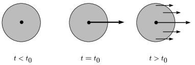
Figure 7: Elastic transition induced by an external heavy-quark current.

It is more conventional to write the above matrix element in terms of an elastic form factor $F_{\rm el}(q^{2})$ depending on the momentum transfer $q^{2}=(p-p^{\prime})^{2}$:

$$\langle\bar{B}(v^{\prime})|\,\bar{b}\,\gamma^{\mu}b\,|\bar{B}(v)\rangle=F_{\rm el}(q^{2})\,(p+p^{\prime})^{\mu}\,,$$ (46)

where $p^{(}\phantom{}{}^{\prime}\phantom{}{}^{)}=m_{B}v^{(}\phantom{}{}^{\prime}\phantom{}{}^{)}$. Comparing this with (44), we find that

$$F_{\rm el}(q^{2})=\xi(v\cdot v^{\prime})\,,\qquad q^{2}=-2m_{B}^{2}(v\cdot v^{\prime}-1)\,.$$ (47)

Because of current conservation, the elastic form factor is normalized to unity at $q^{2}=0$. This condition implies the normalization of the Isgur-Wise function at the kinematic point $v\cdot v^{\prime}=1$, i.e. for $v=v^{\prime}$:

$$\xi(1)=1\,.$$ (48)

It is in accordance with the intuitive argument that the probability for an elastic transition is unity if there is no velocity change. Since for $v=v^{\prime}$ the final-state meson is at rest in the rest frame of the initial meson, the point $v\cdot v^{\prime}=1$ is referred to as the zero-recoil limit.

The heavy-quark flavor symmetry can be used to replace the $b$ quark in the final-state meson by a $c$ quark, thereby turning the $B$ meson into a $D$ meson. Then the scattering process turns into a weak decay process. In the infinite-mass limit, the replacement $b_{v^{\prime}}\to c_{v^{\prime}}$ is a symmetry transformation, under which the effective Lagrangian is invariant. Hence, the matrix element

$${1\over\sqrt{m_{B}m_{D}}}\,\langle D(v^{\prime})|\,\bar{c}_{v^{\prime}}\gamma^{\mu}b_{v}\,|\bar{B}(v)\rangle=\xi(v\cdot v^{\prime})\,(v+v^{\prime})^{\mu}$$ (49)

is still determined by the same function $\xi(v\cdot v^{\prime})$. This is interesting, since in general the matrix element of a flavor-changing current between two pseudoscalar mesons is described by two form factors:

$$\langle D(v^{\prime})|\,\bar{c}\,\gamma^{\mu}b\,|\bar{B}(v)\rangle=f_{+}(q^{2})\,(p+p^{\prime})^{\mu}-f_{-}(q^{2})\,(p-p^{\prime})^{\mu}\,.$$ (50)

Comparing the above two equations, we find that

$$f_{\pm}(q^{2}) = {m_{B}\pm m_{D}\over 2\sqrt{m_{B}m_{D}}}\,\xi(v\cdot v^{\prime})\,,$$

$$q^{2} = m_{B}^{2}+m_{D}^{2}-2m_{B}m_{D}\,v\cdot v^{\prime}\,.$$ (51)

Thus, the heavy-quark flavor symmetry relates two a priori independent form factors to one and the same function. Moreover, the normalization of the Isgur-Wise function at $v\cdot v^{\prime}=1$ now implies a non-trivial normalization of the form factors $f_{\pm}(q^{2})$ at the point of maximum momentum transfer, $q_{\rm max}^{2}=(m_{B}-m_{D})^{2}$:

$$f_{\pm}(q_{\rm max}^{2})={m_{B}\pm m_{D}\over 2\sqrt{m_{B}m_{D}}}\,.$$ (52)

The heavy-quark spin symmetry leads to additional relations among weak decay form factors. It can be used to relate matrix elements involving vector mesons to those involving pseudoscalar mesons. A vector meson with longitudinal polarization is related to a pseudoscalar meson by a rotation of the heavy-quark spin. Hence, the spin-symmetry transformation $c_{v^{\prime}}^{\Uparrow}\to c_{v^{\prime}}^{\Downarrow}$ relates $\bar{B}\to D$ with $\bar{B}\to D^{*}$ transitions. The result of this transformation is $\!{}^{{\bf?}}$

$${1\over\sqrt{m_{B}m_{D^{*}}}}\,\langle D^{*}(v^{\prime},\varepsilon)|\,\bar{c}_{v^{\prime}}\gamma^{\mu}b_{v}\,|\bar{B}(v)\rangle = i\epsilon^{\mu\nu\alpha\beta}\,\varepsilon_{\nu}^{*}\,v^{\prime}_{\alpha}v_{\beta}\,\,\xi(v\cdot v^{\prime})\,,$$

$${1\over\sqrt{m_{B}m_{D^{*}}}}\,\langle D^{*}(v^{\prime},\varepsilon)|\,\bar{c}_{v^{\prime}}\gamma^{\mu}\gamma_{5}\,b_{v}\,|\bar{B}(v)\rangle = \Big{[}\varepsilon^{*\mu}\,(v\cdot v^{\prime}+1)-v^{\prime\mu}\,\varepsilon^{*}\!\cdot v\Big{]}\xi(v\cdot v^{\prime})\,,$$

where $\varepsilon$ denotes the polarization vector of the $D^{*}$ meson. Once again, the matrix elements are completely described in terms of the Isgur-Wise function. Now this is even more remarkable, since in general four form factors, $V(q^{2})$ for the vector current, and $A_{i}(q^{2})$, $i=0,1,2$, for the axial current, are required to parameterize these matrix elements. In the heavy-quark limit, they obey the relations $\!{}^{{\bf?}}$

$${m_{B}+m_{D^{*}}\over 2\sqrt{m_{B}m_{D^{*}}}}\,\xi(v\cdot v^{\prime}) = V(q^{2})=A_{0}(q^{2})=A_{1}(q^{2})$$

$$= \bigg{[}1-{q^{2}\over(m_{B}+m_{D})^{2}}\bigg{]}^{-1}\,A_{1}(q^{2})\,,$$

$$\phantom{\Bigg{[}}q^{2} = m_{B}^{2}+m_{D^{*}}^{2}-2m_{B}m_{D^{*}}\,v\cdot v^{\prime}\,.$$ (54)

Equations (3.1) and (3.1) summarize the relations imposed by heavy-quark symmetry on the weak decay form factors describing the semi-leptonic decay processes $\bar{B}\to D\,\ell\,\bar{\nu}$ and $\bar{B}\to D^{*}\ell\,\bar{\nu}$. These relations are model-independent consequences of QCD in the limit where $m_{b},m_{c}\gg\Lambda_{\rm QCD}$. They play a crucial role in the determination of the CKM matrix element $|V_{cb}|$. In terms of the recoil variable $w=v\cdot v^{\prime}$, the differential semi-leptonic decay rates in the heavy-quark limit become $\!{}^{{\bf?}}$

$${{\rm d}\Gamma(\bar{B}\to D\,\ell\,\bar{\nu})\over{\rm d}w} = {G_{F}^{2}\over 48\pi^{3}}\,|V_{cb}|^{2}\,(m_{B}+m_{D})^{2}\,m_{D}^{3}\,(w^{2}-1)^{3/2}\,\xi^{2}(w)\,,$$

$${{\rm d}\Gamma(\bar{B}\to D^{*}\ell\,\bar{\nu})\over{\rm d}w} = {G_{F}^{2}\over 48\pi^{3}}\,|V_{cb}|^{2}\,(m_{B}-m_{D^{*}})^{2}\,m_{D^{*}}^{3}\,\sqrt{w^{2}-1}\,(w+1)^{2}$$ (55)

$$\times\Bigg{[}1+{4w\over w+1}\,{m_{B}^{2}-2w\,m_{B}m_{D^{*}}+m_{D^{*}}^{2}\over(m_{B}-m_{D^{*}})^{2}}\Bigg{]}\,\xi^{2}(w)\,.$$

These expressions receive symmetry-breaking corrections, since the masses of the heavy quarks are not infinitely large. Perturbative corrections of order $\alpha_{s}^{n}(m_{Q})$ can be calculated order by order in perturbation theory. A more difficult task is to control the non-perturbative power corrections of order $(\Lambda_{\rm QCD}/m_{Q})^{n}$. The HQET provides a systematic framework for analyzing these corrections. For the case of weak-decay form factors the analysis of the $1/m_{Q}$ corrections was performed by Luke $\!{}^{{\bf?}}$. Later, Falk and the present author have analyzed the structure of $1/m_{Q}^{2}$ corrections for both meson and baryon weak decay form factors $\!{}^{{\bf?}}$. We shall not discuss these rather technical issues in detail, but only mention the most important result of Luke’s analysis. It concerns the zero-recoil limit, where an analogue of the Ademollo-Gatto theorem $\!{}^{{\bf?}}$ can be proved. This is Luke’s theorem $\!{}^{{\bf?}}$, which states that the matrix elements describing the leading $1/m_{Q}$ corrections to weak decay amplitudes vanish at zero recoil. This theorem is valid to all orders in perturbation theory $\!{}^{{\bf?},{\bf?},{\bf?}}$. Most importantly, it protects the $\bar{B}\to D^{*}\ell\,\bar{\nu}$ decay rate from receiving first-order $1/m_{Q}$ corrections at zero recoil $\!{}^{{\bf?}}$. [A similar statement is not true for the decay $\bar{B}\to D\,\ell\,\bar{\nu}$. The reason is simple but somewhat subtle. Luke’s theorem protects only those form factors not multiplied by kinematic factors that vanish for $v=v^{\prime}$. By angular momentum conservation, the two pseudoscalar mesons in the decay $\bar{B}\to D\,\ell\,\bar{\nu}$ must be in a relative $p$ wave, and hence the amplitude is proportional to the velocity $|\vec{v}_{D}|$ of the $D$ meson in the $B$-meson rest frame. This leads to a factor $(w^{2}-1)$ in the decay rate. In such a situation, kinematically suppressed form factors can contribute $\!{}^{{\bf?}}$.]

3.2 Short-Distance Corrections

In Sec. 2, we have discussed the first two steps in the construction of the HQET. Integrating out the small components in the heavy-quark fields, a non-local effective action was derived, which was then expanded in a series of local operators. The effective Lagrangian obtained that way correctly reproduces the long-distance physics of the full theory (see Fig. 3). It does not contain the short-distance physics correctly, however. The reason is obvious: a heavy quark participates in strong interactions through its coupling to gluons. These gluons can be soft or hard, i.e. their virtual momenta can be small, of the order of the confinement scale, or large, of the order of the heavy-quark mass. But hard gluons can resolve the spin and flavor quantum numbers of a heavy quark. Their effects lead to a renormalization of the coefficients of the operators in the HQET. A new feature of such short-distance corrections is that through the running coupling constant they induce a logarithmic dependence on the heavy-quark mass $\!{}^{{\bf?}}$. Since $\alpha_{s}(m_{Q})$ is small, these effects can be calculated in perturbation theory.

Consider, as an example, the matrix elements of the vector current $V=\bar{q}\,\gamma^{\mu}Q$. In QCD this current is partially conserved and needs no renormalization. Its matrix elements are free of ultraviolet divergences. Still, these matrix elements have a logarithmic dependence on $m_{Q}$ from the exchange of hard gluons with virtual momenta of the order of the heavy-quark mass. If one goes over to the effective theory by taking the limit $m_{Q}\to\infty$, these logarithms diverge. Consequently, the vector current in the effective theory does require a renormalization $\!{}^{{\bf?}}$. Its matrix elements depend on an arbitrary renormalization scale $\mu$, which separates the regions of short- and long-distance physics. If $\mu$ is chosen such that $\Lambda_{\rm QCD}\ll\mu\ll m_{Q}$, the effective coupling constant in the region between $\mu$ and $m_{Q}$ is small, and perturbation theory can be used to compute the short-distance corrections. These corrections have to be added to the matrix elements of the effective theory, which contain the long-distance physics below the scale $\mu$. Schematically, then, the relation between matrix elements in the full and in the effective theory is

$$\langle\,V(m_{Q})\,\rangle_{\rm QCD}=C_{0}(m_{Q},\mu)\,\langle V_{0}(\mu)\rangle_{\rm HQET}+{C_{1}(m_{Q},\mu)\over m_{Q}}\,\langle V_{1}(\mu)\rangle_{\rm HQET}+\ldots\,,$$ (56)

where we have indicated that matrix elements in the full theory depend on $m_{Q}$, whereas matrix elements in the effective theory are mass-independent, but do depend on the renormalization scale. The Wilson coefficients $C_{i}(m_{Q},\mu)$ are defined by this relation. Order by order in perturbation theory, they can be computed from a comparison of the matrix elements in the two theories. Since the effective theory is constructed to reproduce correctly the low-energy behavior of the full theory, this “matching” procedure is independent of any long-distance physics, such as infrared singularities, non-perturbative effects, and the nature of the external states used in the matrix elements.

The calculation of the coefficient functions in perturbation theory uses the powerful methods of the renormalization group. It is in principle straightforward, yet in practice rather tedious. A comprehensive discussion of most of the existing calculations of short-distance corrections in the HQET can be found in Ref. 18.

3.3 Model-Independent Determination of $|V_{cb}|$

We will now discuss the most important application of the formalism described above in the context of semi-leptonic decays of $B$ mesons. A model-independent determination of the CKM matrix element $|V_{cb}|$ based on heavy-quark symmetry can be obtained by measuring the recoil spectrum of $D^{*}$ mesons produced in $\bar{B}\to D^{*}\ell\,\bar{\nu}$ decays $\!{}^{{\bf?}}$. In the heavy-quark limit, the differential decay rate for this process has been given in (3.1). In order to allow for corrections to that limit, we write

$${{\rm d}\Gamma\over{\rm d}w} = {G_{F}^{2}\over 48\pi^{3}}\,(m_{B}-m_{D^{*}})^{2}\,m_{D^{*}}^{3}\sqrt{w^{2}-1}\,(w+1)^{2}$$ (57)

$$\mbox{}\times\Bigg{[}1+{4w\over w+1}\,{m_{B}^{2}-2w\,m_{B}m_{D^{*}}+m_{D^{*}}^{2}\over(m_{B}-m_{D^{*}})^{2}}\Bigg{]}\,|V_{cb}|^{2}\,{\cal{F}}^{2}(w)\,,$$

where the hadronic form factor ${\cal F}(w)$ coincides with the Isgur-Wise function up to symmetry-breaking corrections of order $\alpha_{s}(m_{Q})$ and $\Lambda_{\rm QCD}/m_{Q}$. The idea is to measure the product $|V_{cb}|\,{\cal F}(w)$ as a function of $w$, and to extract $|V_{cb}|$ from an extrapolation of the data to the zero-recoil point $w=1$, where the $B$ and the $D^{*}$ mesons have a common rest frame. At this kinematic point, heavy-quark symmetry helps us to calculate the normalization ${\cal F}(1)$ with small and controlled theoretical errors. Since the range of $w$ values accessible in this decay is rather small ($1<w<1.5$), the extrapolation can be done using an expansion around $w=1$:

$${\cal F}(w)={\cal F}(1)\,\Big{[}1-\widehat{\varrho}^{2}\,(w-1)+\widehat{c}\,(w-1)^{2}\dots\Big{]}\,.$$ (58)

The slope $\widehat{\varrho}^{2}$ and the curvature $\widehat{c}$, and indeed more generally the complete shape of the form factor, are tightly constrained by analyticity and unitarity requirements $\!{}^{{\bf?},{\bf?}}$. In the long run, the statistics of the experimental results close to zero recoil will be such that these theoretical constraints will not be crucial to get a precision measurement of $|V_{cb}|$. They will, however, enable strong consistency checks.

Figure 8: CLEO data for the product $|V_{cb}|\,{\cal F}(w)$, as extracted from the recoil spectrum in $\bar{B}\to D^{*}\ell\,\bar{\nu}$ decays $\!{}^{{\bf?}}$. The line shows a linear fit to the data.

Measurements of the recoil spectrum have been performed by several experimental groups. Figure 8 shows, as an example, the data reported some time ago by the CLEO Collaboration. The weighted average of the experimental results is $\!{}^{{\bf?}}$

$$|V_{cb}|\,{\cal F}(1)=(35.2\pm 2.6)\times 10^{-3}\,.$$ (59)

Heavy-quark symmetry implies that the general structure of the symmetry-breaking corrections to the form factor at zero recoil is $\!{}^{{\bf?}}$

$${\cal F}(1)=\eta_{A}\,\bigg{(}1+0\times{\Lambda_{\rm QCD}\over m_{Q}}+\mbox{const}\times{\Lambda_{\rm QCD}^{2}\over m_{Q}^{2}}+\dots\bigg{)}\equiv\eta_{A}\,(1+\delta_{1/m^{2}})\,,$$ (60)

where $\eta_{A}$ is a short-distance correction arising from the finite renormalization of the flavor-changing axial current at zero recoil, and $\delta_{1/m^{2}}$ parameterizes second-order (and higher) power corrections. The absence of first-order power corrections at zero recoil is a consequence of Luke’s theorem $\!{}^{{\bf?}}$. The one-loop expression for $\eta_{A}$ has been known for a long time $\!{}^{{\bf?},{\bf?},{\bf?}}$:

$$\eta_{A}=1+{\alpha_{s}(M)\over\pi}\,\bigg{(}{m_{b}+m_{c}\over m_{b}-m_{c}}\,\ln{m_{b}\over m_{c}}-{8\over 3}\bigg{)}\approx 0.96\,.$$ (61)

The scale $M$ in the running coupling constant can be fixed by adopting the prescription of Brodsky, Lepage and Mackenzie (BLM) $\!{}^{{\bf?}}$, where it is identified with the average virtuality of the gluon in the one-loop diagrams that contribute to $\eta_{A}$. If $\alpha_{s}(M)$ is defined in the $\overline{\mbox{\sc ms}}$ scheme, the result is $\!{}^{{\bf?}}$ $M\approx 0.51\sqrt{m_{c}m_{b}}$. Several estimates of higher-order corrections to $\eta_{A}$ have been discussed. A renormalization-group resummation of logarithms of the type $(\alpha_{s}\ln m_{b}/m_{c})^{n}$, $\alpha_{s}(\alpha_{s}\ln m_{b}/m_{c})^{n}$ and $m_{c}/m_{b}(\alpha_{s}\ln m_{b}/m_{c})^{n}$ leads to $\!{}^{{\bf?},{\bf?}}$^-$\!{}^{{\bf?}}$ $\eta_{A}\approx 0.985$. On the other hand, a resummation of “renormalon-chain” contributions of the form $\beta_{0}^{n-1}\alpha_{s}^{n}$, where $\beta_{0}=11-\frac{2}{3}n_{f}$ is the first coefficient of the QCD $\beta$-function, gives $\!{}^{{\bf?}}$ $\eta_{A}\approx 0.945$. Using these partial resummations to estimate the uncertainty gives $\eta_{A}=0.965\pm 0.020$. Recently, Czarnecki has improved this estimate by calculating $\eta_{A}$ at two-loop order $\!{}^{{\bf?}}$. His result, $\eta_{A}=0.960\pm 0.007$, is in excellent agreement with the BLM-improved one-loop expression (61). Here the error is taken to be the size of the two-loop correction.

The analysis of the power corrections is more difficult, since it cannot rely on perturbation theory. Three approaches have been discussed: in the “exclusive approach”, all $1/m_{Q}^{2}$ operators in the HQET are classified and their matrix elements estimated, leading to $\!{}^{{\bf?},{\bf?}}$ $\delta_{1/m^{2}}=-(3\pm 2)\%$; the “inclusive approach” has been used to derive the bound $\delta_{1/m^{2}}<-3\%$, and to estimate that $\!{}^{{\bf?}}$ $\delta_{1/m^{2}}=-(7\pm 3)\%$; the “hybrid approach” combines the virtues of the former two to obtain a more restrictive lower bound on $\delta_{1/m^{2}}$. This leads to $\!{}^{{\bf?}}$ $\delta_{1/m^{2}}=-0.055\pm 0.025$.

Combining the above results, adding the theoretical errors linearly to be conservative, gives

$${\cal F}(1)=0.91\pm 0.03$$ (62)

for the normalization of the hadronic form factor at zero recoil. Thus, the corrections to the heavy-quark limit amount to a moderate decrease of the form factor of about 10%. This can be used to extract from the experimental result (59) the model-independent value

$$|V_{cb}|=(38.7\pm 2.8_{\rm exp}\pm 1.3_{\rm th})\times 10^{-3}\,.$$ (63)

3.4 Measurements of $\bar{B}\to D^{*}\ell\,\bar{\nu}$ and $\bar{B}\to D\,\ell\,\bar{\nu}$ Form Factors and Tests of Heavy-Quark Symmetry

We have discussed earlier in this section that heavy-quark symmetry implies relations between the semi-leptonic form factors of heavy mesons. They receive symmetry-breaking corrections, which can be estimated using the HQET. The extent to which these relations hold can be tested experimentally by comparing the different form factors describing the decays $\bar{B}\to D^{(*)}\ell\,\bar{\nu}$ at the same value of $w$.

When the lepton mass is neglected, the differential decay distributions in $\bar{B}\to D^{*}\ell\,\bar{\nu}$ decays can be parameterized by three helicity amplitudes, or equivalently by three independent combinations of form factors. It has been suggested that a good choice for three such quantities should be inspired by the heavy-quark limit $\!{}^{{\bf?},{\bf?}}$. One thus defines a form factor $h_{A1}(w)$, which up to symmetry-breaking corrections coincides with the Isgur-Wise function, and two form-factor ratios

$$R_{1}(w) = \bigg{[}1-{q^{2}\over(m_{B}+m_{D^{*}})^{2}}\bigg{]}\,{V(q^{2})\over A_{1}(q^{2})}\,,$$

$$R_{2}(w) = \bigg{[}1-{q^{2}\over(m_{B}+m_{D^{*}})^{2}}\bigg{]}\,{A_{2}(q^{2})\over A_{1}(q^{2})}\,.$$ (64)

The relation between $w$ and $q^{2}$ has been given in (3.1). This definition is such that in the heavy-quark limit $R_{1}(w)=R_{2}(w)=1$ independently of $w$.

To extract the functions $h_{A1}(w)$, $R_{1}(w)$ and $R_{2}(w)$ from experimental data is a complicated task. However, HQET-based calculations suggest that the $w$ dependence of the form-factor ratios, which is induced by symmetry-breaking effects, is rather mild $\!{}^{{\bf?}}$. Moreover, the form factor $h_{A1}(w)$ is expected to have a nearly linear shape over the accessible $w$ range. This motivates to introduce three parameters $\varrho_{A1}^{2}$, $R_{1}$ and $R_{2}$ by

$$h_{A1}(w) \approx {\cal F}(1)\,\Big{[}1-\varrho_{A1}^{2}(w-1)\Big{]}\,,$$

$$R_{1}(w) \approx R_{1}\,,\qquad R_{2}(w)\approx R_{2}\,,$$ (65)

where ${\cal F}(1)=0.91\pm 0.03$ from (62). The CLEO Collaboration has extracted these three parameters from an analysis of the angular distributions in $\bar{B}\to D^{*}\ell\,\bar{\nu}$ decays $\!{}^{{\bf?}}$. The results are

$$\varrho_{A1}^{2}=0.91\pm 0.16\,,\qquad R_{1}=1.18\pm 0.32\,,\qquad R_{2}=0.71\pm 0.23\,.$$ (66)

Using the HQET, one obtains an essentially model-independent prediction for the symmetry-breaking corrections to $R_{1}$, whereas the corrections to $R_{2}$ are somewhat model dependent. To good approximation $\!{}^{{\bf?}}$

$$R_{1} \approx 1+{4\alpha_{s}(m_{c})\over 3\pi}+{\bar{\Lambda}\over 2m_{c}}\approx 1.3\pm 0.1\,,$$

$$R_{2} \approx 1-\kappa\,{\bar{\Lambda}\over 2m_{c}}\approx 0.8\pm 0.2\,,$$ (67)

with $\kappa\approx 1$ from QCD sum rules $\!{}^{{\bf?}}$. Here $\bar{\Lambda}$ is the “binding energy” as defined in (28). Theoretical calculations $\!{}^{{\bf?},{\bf?}}$ as well as phenomenological analyses $\!{}^{{\bf?},{\bf?}}$ suggest that $\bar{\Lambda}\approx 0.45$–0.65 GeV is the appropriate value to be used in one-loop calculations. A quark-model calculation of $R_{1}$ and $R_{2}$ gives results similar to the HQET predictions $\!{}^{{\bf?}}$: $R_{1}\approx 1.15$ and $R_{2}\approx 0.91$. The experimental data confirm the theoretical prediction that $R_{1}>1$ and $R_{2}<1$, although the errors are still large.

Heavy-quark symmetry has also been tested by comparing the form factor ${\cal F}(w)$ in $\bar{B}\to D^{*}\ell\,\bar{\nu}$ decays with the corresponding form factor ${\cal G}(w)$ governing $\bar{B}\to D\,\ell\,\bar{\nu}$ decays. The theoretical prediction $\!{}^{{\bf?},{\bf?}}$

$$\frac{{\cal G}(1)}{{\cal F}(1)}=1.08\pm 0.06$$ (68)

compares well with the experimental results for this ratio: $0.99\pm 0.19$ reported by the CLEO Collaboration $\!{}^{{\bf?}}$, and $0.87\pm 0.30$ reported by the ALEPH Collaboration $\!{}^{{\bf?}}$. In these analyses, it has also been tested that within experimental errors the shape of the two form factors agrees over the entire range of $w$ values.

The results of the analyses described above are very encouraging. Within errors, the experiments confirm the HQET predictions, starting to test them at the level of symmetry-breaking corrections.

4 Inclusive Decay Rates

Inclusive decay rates determine the probability of the decay of a particle into the sum of all possible final states with a given set of global quantum numbers. An example is provided by the inclusive semi-leptonic decay rate of the $B$ meson, $\Gamma(\bar{B}\to X\,\ell\,\bar{\nu})$, where the final state consists of a lepton-neutrino pair accompanied by any number of hadrons. Here we shall discuss the theoretical description of inclusive decays of hadrons containing a heavy quark $\!{}^{{\bf?}}$^-$\!{}^{{\bf?}}$. From a theoretical point of view such decays have two advantages: first, bound-state effects related to the initial state, such as the “Fermi motion” of the heavy quark inside the hadron $\!{}^{{\bf?},{\bf?}}$, can be accounted for in a systematic way using the heavy-quark expansion; secondly, the fact that the final state consists of a sum over many hadronic channels eliminates bound-state effects related to the properties of individual hadrons. This second feature is based on the hypothesis of quark-hadron duality, which is an important concept in QCD phenomenology. The assumption of duality is that cross sections and decay rates, which are defined in the physical region (i.e. the region of time-like momenta), are calculable in QCD after a “smearing” or “averaging” procedure has been applied $\!{}^{{\bf?}}$. In semi-leptonic decays, it is the integration over the lepton and neutrino phase space that provides a smearing over the invariant hadronic mass of the final state (so-called global duality). For non-leptonic decays, on the other hand, the total hadronic mass is fixed, and it is only the fact that one sums over many hadronic states that provides an averaging (so-called local duality). Clearly, local duality is a stronger assumption than global duality. It is important to stress that quark-hadron duality cannot yet be derived from first principles; still, it is a necessary assumption for many applications of QCD. The validity of global duality has been tested experimentally using data on hadronic $\tau$ decays $\!{}^{{\bf?}}$.

Using the optical theorem, the inclusive decay width of a hadron $H_{b}$ containing a $b$ quark can be written in the form

$$\Gamma(H_{b}\to X)=\frac{1}{m_{H_{b}}}\,\mbox{Im}\,\langle H_{b}|\,{\bf T}\,|H_{b}\rangle\,,$$ (69)

where the transition operator ${\bf T}$ is given by

$${\bf T}=i\!\int{\rm d}^{4}x\,T\{\,{\cal L}_{\rm eff}(x),{\cal L}_{\rm eff}(0)\,\}\,.$$ (70)

Inserting a complete set of states inside the time-ordered product, we recover the standard expression

$$\Gamma(H_{b}\to X)={1\over 2m_{H_{b}}}\,\sum_{X}\,(2\pi)^{4}\,\delta^{4}(p_{H}-p_{X})\,|\langle X|\,{\cal L}_{\rm eff}\,|H_{b}\rangle|^{2}$$ (71)

for the decay rate. For the case of semi-leptonic and non-leptonic decays, ${\cal L}_{\rm eff}$ is the effective weak Lagrangian given in (4), which in practice is corrected for short-distance effects $\!{}^{{\bf?},{\bf?},{\bf?}}$^-$\!{}^{{\bf?}}$ arising from the exchange of gluons with virtualities between $m_{W}$ and $m_{b}$. If some quantum numbers of the final states $X$ are specified, the sum over intermediate states is to be restricted appropriately. In the case of the inclusive semi-leptonic decay rate, for instance, the sum would include only those states $X$ containing a lepton-neutrino pair.

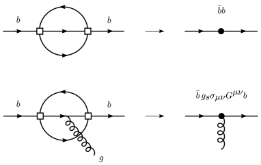
Figure 9: Perturbative contributions to the transition operator ${\bf T}$ (left), and the corresponding operators in the OPE (right). The open squares represent a four-fermion interaction of the effective Lagrangian ${\cal L}_{\rm eff}$, while the black circles represent local operators in the OPE.

In perturbation theory, some contributions to the transition operator are given by the two-loop diagrams shown on the left-hand side in Fig. 9. Because of the large mass of the $b$ quark, the momenta flowing through the internal propagator lines are large. It is thus possible to construct an OPE for the transition operator, in which ${\bf T}$ is represented as a series of local operators containing the heavy-quark fields. The operator with the lowest dimension, $d=3$, is $\bar{b}b$. It arises by contracting the internal lines of the first diagram. The only gauge-invariant operator with dimension 4 is $\bar{b}\,i\hbox to0.0pt{\,/\hss}D\,b$; however, the equations of motion imply that between physical states this operator can be replaced by $m_{b}\bar{b}b$. The first operator that is different from $\bar{b}b$ has dimension 5 and contains the gluon field. It is given by $\bar{b}\,g_{s}\sigma_{\mu\nu}G^{\mu\nu}b$. This operator arises from diagrams in which a gluon is emitted from one of the internal lines, such as the second diagram shown in Fig. 9. For dimensional reasons, the matrix elements of such higher-dimensional operators are suppressed by inverse powers of the heavy-quark mass. Thus, any inclusive decay rate of a hadron $H_{b}$ can be written as $\!{}^{{\bf?}}$^-$\!{}^{{\bf?}}$

$$\Gamma(H_{b}\to X_{f})={G_{F}^{2}m_{b}^{5}\over 192\pi^{3}}\,\bigg{\{}c_{3}^{f}\,\langle\bar{b}b\rangle_{H}+c_{5}^{f}\,{\langle\bar{b}\,g_{s}\sigma_{\mu\nu}G^{\mu\nu}b\rangle_{H}\over m_{b}^{2}}+\dots\bigg{\}}\,,$$ (72)

where the prefactor arises naturally from the loop integrations, $c_{n}^{f}$ are calculable coefficient functions (which also contain the relevant CKM matrix elements) depending on the quantum numbers $f$ of the final state, and $\langle O\rangle_{H}$ are the (normalized) forward matrix elements of local operators, for which we use the short-hand notation

$$\langle O\rangle_{H}={1\over 2m_{H_{b}}}\,\langle H_{b}|\,O\,|H_{b}\rangle\,.$$ (73)

In the next step, these matrix elements are systematically expanded in powers of $1/m_{b}$, using the technology of the HQET. The result is $\!{}^{{\bf?},{\bf?},{\bf?}}$

$$\langle\bar{b}b\rangle_{H} = 1-{\mu_{\pi}^{2}(H_{b})-\mu_{G}^{2}(H_{b})\over 2m_{b}^{2}}+O(1/m_{b}^{3})\,,$$

$$\langle\bar{b}\,g_{s}\sigma_{\mu\nu}G^{\mu\nu}b\rangle_{H} = 2\mu_{G}^{2}(H_{b})+O(1/m_{b})\,,$$ (74)

where we have defined the HQET matrix elements

$$\mu_{\pi}^{2}(H_{b}) = {1\over 2m_{H_{b}}}\,\langle H_{b}(v)|\,\bar{b}_{v}\,(i\vec{D})^{2}\,b_{v}\,|H_{b}(v)\rangle\,,$$

$$\mu_{G}^{2}(H_{b}) = {1\over 2m_{H_{b}}}\,\langle H_{b}(v)|\,\bar{b}_{v}{g_{s}\over 2}\sigma_{\mu\nu}G^{\mu\nu}b_{v}\,|H_{b}(v)\rangle\,.$$ (75)

Here $(i\vec{D})^{2}=(iv\cdot D)^{2}-(iD)^{2}$; in the rest frame, this is the square of the operator for the spatial momentum of the heavy quark. Inserting these results into (72) yields

$$\Gamma(H_{b}\to X_{f})={G_{F}^{2}m_{b}^{5}\over 192\pi^{3}}\,\bigg{\{}c_{3}^{f}\,\bigg{(}1-{\mu_{\pi}^{2}(H_{b})-\mu_{G}^{2}(H_{b})\over 2m_{b}^{2}}\bigg{)}+2c_{5}^{f}\,{\mu_{G}^{2}(H_{b})\over m_{b}^{2}}+\dots\bigg{\}}\,.$$ (76)

It is instructive to understand the appearance of the “kinetic energy” contribution $\mu_{\pi}^{2}$, which is the gauge-covariant extension of the square of the $b$-quark momentum inside the heavy hadron. This contribution is the field-theory analogue of the Lorentz factor $(1-\vec{v}_{b}^{\,2})^{1/2}\simeq 1-\vec{k}^{\,2}/2m_{b}^{2}$, in accordance with the fact that the lifetime, $\tau=1/\Gamma$, for a moving particle increases due to time dilation.

The main result of the heavy-quark expansion for inclusive decay rates is the observation that the free quark decay (i.e. the parton model) provides the first term in a systematic $1/m_{b}$ expansion $\!{}^{{\bf?}}$. For dimensional reasons, the corresponding rate is proportional to the fifth power of the $b$-quark mass. The non-perturbative corrections, which arise from bound-state effects inside the $B$ meson, are suppressed by at least two powers of the heavy-quark mass, i.e. they are of relative order $(\Lambda_{\rm QCD}/m_{b})^{2}$. Note that the absence of first-order power corrections is a consequence of the equations of motion, as there is no independent gauge-invariant operator of dimension 4 that could appear in the OPE. The fact that bound-state effects in inclusive decays are strongly suppressed explains a posteriori the success of the parton model in describing such processes $\!{}^{{\bf?},{\bf?}}$.

The hadronic matrix elements appearing in the heavy-quark expansion (76) can be determined to some extent from the known masses of heavy hadron states. For the $B$ meson, one finds that

$$\mu_{\pi}^{2}(B) = -\lambda_{1}=(0.3\pm 0.2)~{}\mbox{GeV}^{2}\,,$$

$$\mu_{G}^{2}(B) = 3\lambda_{2}\approx 0.36~{}\mbox{GeV}^{2}\,,$$ (77)

where $\lambda_{1}$ and $\lambda_{2}$ are the parameters appearing in the mass formula (32). For the ground-state baryon $\Lambda_{b}$, in which the light constituents have total spin zero, it follows that

$$\mu_{G}^{2}(\Lambda_{b})=0\,,$$ (78)

while the matrix element $\mu_{\pi}^{2}(\Lambda_{b})$ obeys the relation

$$(m_{\Lambda_{b}}-m_{\Lambda_{c}})-(\overline{m}_{B}-\overline{m}_{D})=\Big{[}\mu_{\pi}^{2}(B)-\mu_{\pi}^{2}(\Lambda_{b})\Big{]}\,\bigg{(}{1\over 2m_{c}}-{1\over 2m_{b}}\bigg{)}+O(1/m_{Q}^{2})\,,$$ (79)

where $\overline{m}_{B}$ and $\overline{m}_{D}$ denote the spin-averaged masses introduced in connection with (41). The above relation implies

$$\mu_{\pi}^{2}(B)-\mu_{\pi}^{2}(\Lambda_{b})=(0.01\pm 0.03)~{}\mbox{GeV}^{2}\,.$$ (80)

What remains to be calculated, then, is the coefficient functions $c_{n}^{f}$ for a given inclusive decay channel.

To illustrate this general formalism, we discuss as an example the determination of $|V_{cb}|$ from inclusive semi-leptonic $B$ decays. In this case the short-distance coefficients in the general expression (76) are given by $\!{}^{{\bf?}}$^-$\!{}^{{\bf?}}$

$$c_{3}^{\rm SL} = |V_{cb}|^{2}\Big{[}1-8x^{2}+8x^{6}-x^{8}-12x^{4}\ln x^{2}+O(\alpha_{s})\Big{]}\,,$$

$$c_{5}^{\rm SL} = -6|V_{cb}|^{2}(1-x^{2})^{4}\,.$$ (81)

Here $x=m_{c}/m_{b}$, and $m_{b}$ and $m_{c}$ are the masses of the $b$ and $c$ quarks, defined to a given order in perturbation theory $\!{}^{{\bf?}}$. The $O(\alpha_{s})$ terms in $c_{3}^{\rm SL}$ are known exactly $\!{}^{{\bf?}}$, and reliable estimates exist for the $O(\alpha_{s}^{2})$ corrections $\!{}^{{\bf?}}$. The theoretical uncertainties in this determination of $|V_{cb}|$ are quite different from those entering the analysis of exclusive decays. The main sources are the dependence on the heavy-quark masses, higher-order perturbative corrections, and above all the assumption of global quark-hadron duality. A conservative estimate of the total theoretical error on the extracted value of $|V_{cb}|$ yields $\!{}^{{\bf?}}$

$$|V_{cb}|=(0.040\pm 0.003)\bigg{[}{\hbox{B}_{\rm SL}\over 10.5\%}\bigg{]}^{1/2}\bigg{[}\frac{1.6\,\mbox{ps}}{\tau_{B}}\bigg{]}^{1/2}=(40\pm 1_{\rm exp}\pm 3_{\rm th})\times 10^{-3}\,.$$ (82)

The value of $|V_{cb}|$ extracted from the inclusive semi-leptonic width is in excellent agreement with the value in (63) obtained from the analysis of the exclusive decay $\bar{B}\to D^{*}\ell\,\bar{\nu}$. This agreement is gratifying given the differences of the methods used, and it provides an indirect test of global quark-hadron duality. Combining the two measurements gives the final result

$$|V_{cb}|=0.039\pm 0.002\,.$$ (83)

After $V_{ud}$ and $V_{us}$, this is the third-best known entry in the CKM matrix.

5 Rare $B$ Decays and Determination of the Weak Phase $\gamma$

The main objectives of the $B$ factories are to explore the physics of CP violation, to determine the flavor parameters of the electroweak theory, and to probe for physics beyond the Standard Model. This will test the CKM mechanism, which predicts that all CP violation results from a single complex phase in the quark mixing matrix. Facing the announcement of evidence for a CP asymmetry in the decays $B\to J/\psi\,K_{S}$ by the CDF Collaboration $\!{}^{{\bf?}}$, the confirmation of direct CP violation in $K\to\pi\pi$ decays by the KTeV and NA48 groups $\!{}^{{\bf?},{\bf?}}$, and the successful start of the $B$ factories at SLAC and KEK, the year 1999 has been an important step towards achieving this goal.

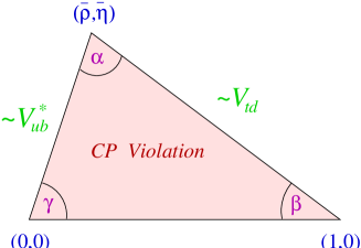
Figure 10: The rescaled unitarity triangle representing the relation $1+\frac{V_{ub}^{*}V_{ud}}{V_{cb}^{*}V_{cd}}+\frac{V_{tb}^{*}V_{td}}{V_{cb}^{*}V_{cd}}=0$. The apex is determined by the Wolfenstein parameters $(\bar{\rho},\bar{\eta})$. The area of the triangle is proportional to the strength of CP violation in the Standard Model.

The determination of the sides and angles of the “unitarity triangle” $V_{ub}^{*}V_{ud}+V_{cb}^{*}V_{cd}+V_{tb}^{*}V_{td}=0$ depicted in Fig. 10 plays a central role in the $B$ factory program. Adopting the standard phase conventions for the CKM matrix, only the two smallest elements in this relation, $V_{ub}^{*}$ and $V_{td}$, have non-vanishing imaginary parts (to an excellent approximation). In the Standard Model the angle $\beta=-\mbox{arg}(V_{td})$ can be determined in a theoretically clean way by measuring the mixing-induced CP asymmetry in the decays $B\to J/\psi\,K_{S}$. The preliminary CDF result implies $\!{}^{{\bf?}}$ $\sin 2\beta=0.79_{-0.44}^{+0.41}$. The angle $\gamma=\mbox{arg}(V_{ub}^{*})$, or equivalently the combination $\alpha=180^{\circ}-\beta-\gamma$, is much harder to determine $\!{}^{{\bf?}}$. Recently, there has been significant progress in the theoretical understanding of the hadronic decays $B\to\pi K$, and methods have been developed to extract information on $\gamma$ from rate measurements for these processes. Here we discuss the charged modes $B^{\pm}\to\pi K$, which from a theoretical perspective are particularly clean.

In the Standard Model, the main contributions to the decay amplitudes for the rare processes $B\to\pi K$ are due to the penguin-induced flavor-changing neutral current (FCNC) transitions $\bar{b}\to\bar{s}q\bar{q}$, which exceed a small, Cabibbo-suppressed $\bar{b}\to\bar{u}u\bar{s}$ contribution from $W$-boson exchange. The weak phase $\gamma$ enters through the interference of these two (“penguin” and “tree”) contributions. Because of a fortunate interplay of isospin, Fierz and flavor symmetries, the theoretical description of the charged modes $B^{\pm}\to\pi K$ is very clean despite the fact that these are exclusive non-leptonic decays $\!{}^{{\bf?}}$^-$\!{}^{{\bf?}}$. Without any dynamical assumption, the hadronic uncertainties in the description of the interference terms relevant to the determination of $\gamma$ are of relative magnitude $O(\lambda^{2})$ or $O(\epsilon_{\rm SU(3)}/N_{c})$, where $\lambda=\sin\theta_{C}\approx 0.22$ is a measure of Cabibbo suppression, $\epsilon_{\rm SU(3)}\sim 20\%$ is the typical size of SU(3) breaking, and the factor $1/N_{c}$ indicates that the corresponding terms vanish in the factorization approximation. Factorizable SU(3) breaking can be accounted for in a straightforward way.

Recently, the accuracy of this description has been further improved when it was shown that non-leptonic $B$ decays into two light mesons, such as $B\to\pi K$ and $B\to\pi\pi$, admit a systematic heavy-quark expansion $\!{}^{{\bf?}}$. To leading order in $1/m_{b}$, but to all orders in perturbation theory, the decay amplitudes for these processes can be calculated from first principles without recourse to phenomenological models. The QCD factorization theorem proved in Ref. 122 improves upon the phenomenological approach of “generalized factorization” $\!{}^{{\bf?}}$, which emerges as the leading term in the heavy-quark limit. With the help of this theorem, the irreducible theoretical uncertainties in the description of the $B^{\pm}\to\pi K$ decay amplitudes can be reduced by an extra factor of $O(1/m_{b})$, rendering their analysis essentially model independent. As a consequence of this fact, and because they are dominated by FCNC transitions, the decays $B^{\pm}\to\pi K$ offer a sensitive probe to physics beyond the Standard Model $\!{}^{{\bf?},{\bf?}}$^-$\!{}^{{\bf?}}$, much in the same way as the “classical” FCNC processes $B\to X_{s}\gamma$ or $B\to X_{s}\,\ell^{+}\ell^{-}$.

5.1 Theory of $B^{\pm}\to\pi K$ Decays

The hadronic decays $B\to\pi K$ are mediated by a low-energy effective weak Hamiltonian $\!{}^{{\bf?}}$, whose operators allow for three different classes of flavor topologies: QCD penguins, trees, and electroweak penguins. In the Standard Model the weak couplings associated with these topologies are known. From the measured branching ratios one can deduce that QCD penguins dominate the $B\to\pi K$ decay amplitudes $\!{}^{{\bf?}}$, whereas trees and electroweak penguins are subleading and of a similar strength $\!{}^{{\bf?}}$. The theoretical description of the two charged modes $B^{\pm}\to\pi^{\pm}K^{0}$ and $B^{\pm}\to\pi^{0}K^{\pm}$ exploits the fact that the amplitudes for these processes differ in a pure isospin amplitude, $A_{3/2}$, defined as the matrix element of the isovector part of the effective Hamiltonian between a $B$ meson and the $\pi K$ isospin eigenstate with $I=\frac{3}{2}$. In the Standard Model the parameters of this amplitude are determined, up to an overall strong phase $\phi$, in the limit of SU(3) flavor symmetry $\!{}^{{\bf?}}$. Using the QCD factorization theorem the SU(3)-breaking corrections can be calculated in a model-independent way up to non-factorizable terms that are power-suppressed in $1/m_{b}$ and vanish in the heavy-quark limit.

A convenient parameterization of the non-leptonic decay amplitudes ${\cal A}_{+0}\equiv{\cal A}(B^{+}\to\pi^{+}K^{0})$ and ${\cal A}_{0+}\equiv-\sqrt{2}\,{\cal A}(B^{+}\to\pi^{0}K^{+})$ is $\!{}^{{\bf?}}$

$${\cal A}_{+0} = P\,(1-\varepsilon_{a}\,e^{i\gamma}e^{i\eta})\,,$$

$${\cal A}_{0+} = P\Big{[}1-\varepsilon_{a}\,e^{i\gamma}e^{i\eta}-\varepsilon_{3/2}\,e^{i\phi}(e^{i\gamma}-\delta_{\rm EW})\Big{]}\,,$$ (84)

where $P$ is the dominant penguin amplitude defined as the sum of all terms in the $B^{+}\to\pi^{+}K^{0}$ amplitude not proportional to $e^{i\gamma}$, $\eta$ and $\phi$ are strong phases, and $\varepsilon_{a}$, $\varepsilon_{3/2}$ and $\delta_{\rm EW}$ are real hadronic parameters. The weak phase $\gamma$ changes sign under a CP transformation, whereas all other parameters stay invariant.

Based on a naive quark-diagram analysis one would not expect the $B^{+}\to\pi^{+}K^{0}$ amplitude to receive a contribution from $\bar{b}\to\bar{u}u\bar{s}$ tree topologies; however, such a contribution can be induced through final-state rescattering or annihilation contributions $\!{}^{{\bf?}}$^-$\!{}^{{\bf?}}$. They are parameterized by $\varepsilon_{a}=O(\lambda^{2})$. In the heavy-quark limit this parameter can be calculated and is found to be very small  $\!{}^{{\bf?}}$: $\varepsilon_{a}\approx-2\%$. In the future, it will be possible to put upper and lower bounds on $\varepsilon_{a}$ by comparing the CP-averaged branching ratios for the decays $\!{}^{{\bf?}}$ $B^{\pm}\to\pi^{\pm}K^{0}$ and $B^{\pm}\to K^{\pm}\bar{K}^{0}$. Below we assume $|\varepsilon_{a}|\leq 0.1$; however, our results will be almost insensitive to this assumption.

The terms proportional to $\varepsilon_{3/2}$ in (5.1) parameterize the isospin amplitude $A_{3/2}$. The weak phase $e^{i\gamma}$ enters through the tree process $\bar{b}\to\bar{u}u\bar{s}$, whereas the quantity $\delta_{\rm EW}$ describes the effects of electroweak penguins. The parameter $\varepsilon_{3/2}$ measures the relative strength of tree and QCD penguin contributions. Information about it can be derived by using SU(3) flavor symmetry to relate the tree contribution to the isospin amplitude $A_{3/2}$ to the corresponding contribution in the decay $B^{+}\to\pi^{+}\pi^{0}$. Since the final state $\pi^{+}\pi^{0}$ has isospin $I=2$, the amplitude for this process does not receive any contribution from QCD penguins. Moreover, electroweak penguins in $\bar{b}\to\bar{d}q\bar{q}$ transitions are negligibly small. We define a related parameter $\bar{\varepsilon}_{3/2}$ by writing

$$\varepsilon_{3/2}=\bar{\varepsilon}_{3/2}\sqrt{1-2\varepsilon_{a}\cos\eta\cos\gamma+\varepsilon_{a}^{2}}\,,$$ (85)

so that the two quantities agree in the limit $\varepsilon_{a}\to 0$. In the SU(3) limit this new parameter can be determined experimentally form the relation $\!{}^{{\bf?}}$

$$\bar{\varepsilon}_{3/2}=R_{1}\left|\frac{V_{us}}{V_{ud}}\right|\left[\frac{2\mbox{B}(B^{\pm}\to\pi^{\pm}\pi^{0})}{\mbox{B}(B^{\pm}\to\pi^{\pm}K^{0})}\right]^{1/2}.$$ (86)

SU(3)-breaking corrections are described by the factor $R_{1}=1.22\pm 0.05$, which can be calculated in a model-independent way using the QCD factorization theorem for non-leptonic decays $\!{}^{{\bf?}}$. The quoted error is an estimate of the theoretical uncertainty due to corrections of $O(\frac{1}{N_{c}}\frac{m_{s}}{m_{b}})$. Using preliminary data reported by the CLEO Collaboration $\!{}^{{\bf?}}$ to evaluate the ratio of the CP-averaged branching ratios in (86), we obtain

$$\bar{\varepsilon}_{3/2}=0.21\pm 0.06_{\rm exp}\pm 0.01_{\rm th}\,.$$ (87)

With a better measurement of the branching ratios the uncertainty in $\bar{\varepsilon}_{3/2}$ will be reduced significantly.

Finally, the parameter

$$\delta_{\rm EW} = R_{2}\,\left|\frac{V_{cb}^{*}V_{cs}}{V_{ub}^{*}V_{us}}\right|\,\frac{\alpha}{8\pi}\,\frac{x_{t}}{\sin^{2}\!\theta_{W}}\left(1+\frac{3\ln x_{t}}{x_{t}-1}\right)$$ (88)

$$= (0.64\pm 0.09)\times\frac{0.085}{|V_{ub}/V_{cb}|}\,,$$

with $x_{t}=(m_{t}/m_{W})^{2}$, describes the ratio of electroweak penguin and tree contributions to the isospin amplitude $A_{3/2}$. In the SU(3) limit it is calculable in terms of Standard Model parameters $\!{}^{{\bf?},{\bf?}}$. SU(3)-breaking as well as small electromagnetic corrections are accounted for by the quantity $\!{}^{{\bf?},{\bf?}}$ $R_{2}=0.92\pm 0.09$. The error quoted in (88) includes the uncertainty in the top-quark mass.

Important observables in the study of the weak phase $\gamma$ are the ratio of the CP-averaged branching ratios in the two $B^{\pm}\to\pi K$ decay modes,

$$R_{*}=\frac{\mbox{B}(B^{\pm}\to\pi^{\pm}K^{0})}{2\mbox{B}(B^{\pm}\to\pi^{0}K^{\pm})}=0.75\pm 0.28\,,$$ (89)

and a particular combination of the direct CP asymmetries,

$$\widetilde{A}=\frac{A_{\rm CP}(B^{\pm}\to\pi^{0}K^{\pm})}{R_{*}}-A_{\rm CP}(B^{\pm}\to\pi^{\pm}K^{0})=-0.52\pm 0.42\,.$$ (90)

The experimental values of these quantities are derived using preliminary data reported by the CLEO Collaboration $\!{}^{{\bf?}}$. The theoretical expressions for $R_{*}$ and $\widetilde{A}$ obtained using the parameterization in (5.1) are

$$R_{*}^{-1} = 1+2\bar{\varepsilon}_{3/2}\cos\phi\,(\delta_{\rm EW}-\cos\gamma)$$

$$\mbox{}+\bar{\varepsilon}_{3/2}^{2}(1-2\delta_{\rm EW}\cos\gamma+\delta_{\rm EW}^{2})\!+\!O(\bar{\varepsilon}_{3/2}\varepsilon_{a})\,,$$

$$\widetilde{A} = 2\bar{\varepsilon}_{3/2}\sin\gamma\sin\phi+O(\bar{\varepsilon}_{3/2}\varepsilon_{a})\,.$$ (91)

Note that the rescattering effects described by $\varepsilon_{a}$ are suppressed by a factor of $\bar{\varepsilon}_{3/2}$ and thus reduced to the percent level. Explicit expressions for these contributions can be found in Ref. 121.

5.2 Lower Bound on $\gamma$ and Constraint in the $(\bar{\rho},\bar{\eta})$ Plane

There are several strategies for exploiting the above relations. From a measurement of the ratio $R_{*}$ alone a bound on $\cos\gamma$ can be derived, implying a non-trivial constraint on the Wolfenstein parameters $\bar{\rho}$ and $\bar{\eta}$ defining the apex of the unitarity triangle $\!{}^{{\bf?}}$. Only CP-averaged branching ratios are needed for this purpose. Varying the strong phases $\phi$ and $\eta$ independently we first obtain an upper bound on the inverse of $R_{*}$. Keeping terms of linear order in $\varepsilon_{a}$ yields $\!{}^{{\bf?}}$

$$R_{*}^{-1}\leq\left(1+\bar{\varepsilon}_{3/2}\,|\delta_{\rm EW}-\cos\gamma|\right)^{2}+\bar{\varepsilon}_{3/2}^{2}\sin^{2}\!\gamma+2\bar{\varepsilon}_{3/2}|\varepsilon_{a}|\sin^{2}\!\gamma\,.$$ (92)

Provided $R_{*}$ is significantly smaller than 1, this bound implies an exclusion region for $\cos\gamma$ which becomes larger the smaller the values of $R_{*}$ and $\bar{\varepsilon}_{3/2}$ are. It is convenient to consider instead of $R_{*}$ the related quantity $\!{}^{{\bf?}}$

$$X_{R}=\frac{\sqrt{R_{*}^{-1}}-1}{\bar{\varepsilon}_{3/2}}=0.72\pm 0.98_{\rm exp}\pm 0.03_{\rm th}\,.$$ (93)

Because of the theoretical factor $R_{1}$ entering the definition of $\bar{\varepsilon}_{3/2}$ in (86) this is, strictly speaking, not an observable. However, the theoretical uncertainty in $X_{R}$ is so much smaller than the present experimental error that it can be ignored for all practical purposes. The advantage of presenting our results in terms of $X_{R}$ rather than $R_{*}$ is that the leading dependence on $\bar{\varepsilon}_{3/2}$ cancels out, leading to the simple bound $|X_{R}|\leq|\delta_{\rm EW}-\cos\gamma|+O(\bar{\varepsilon}_{3/2},\varepsilon_{a})$.

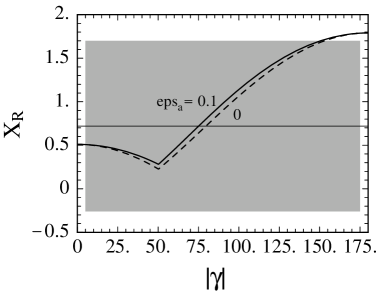
Figure 11: Theoretical upper bound on the ratio $X_{R}$ versus $|\gamma|$ for $\varepsilon_{a}=0.1$ (solid line) and $\varepsilon_{a}=0$ (dashed line). The horizontal line and band show the current experimental value with its $1\sigma$ variation.

In Fig. 11 we show the upper bound on $X_{R}$ as a function of $|\gamma|$, obtained by varying the input parameters in the intervals $0.15\leq\bar{\varepsilon}_{3/2}\leq 0.27$ and $0.49\leq\delta_{\rm EW}\leq 0.79$ (corresponding to using $|V_{ub}/V_{cb}|=0.085\pm 0.015$ in (88)). Note that the effect of the rescattering contribution parameterized by $\varepsilon_{a}$ is very small. The gray band shows the current value of $X_{R}$, which still has too large an error to provide any useful information on $\gamma$. The situation may change, however, once a more precise measurement of $X_{R}$ will become available. For instance, if the current central value $X_{R}=0.72$ were confirmed, it would imply the bound $|\gamma|>75^{\circ}$, marking a significant improvement over the indirect limit $|\gamma|>37^{\circ}$ inferred from the global analysis of the unitarity triangle including information from $K$–$\bar{K}$ mixing $\!{}^{{\bf?}}$.

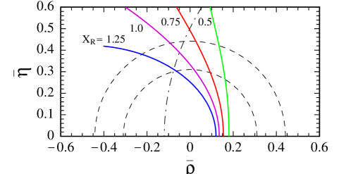
Figure 12: Theoretical constraints on the Wolfenstein parameters $(\bar{\rho},\bar{\eta})$ implied by a measurement of the ratio $X_{R}$ in $B^{\pm}\to\pi K$ decays (solid lines), semi-leptonic $B$ decays (dashed circles), and $B_{d,s}$–$\bar{B}_{d,s}$ mixing (dashed-dotted line).

So far, we have used the inequality (92) to derive a lower bound on $|\gamma|$. However, a large part of the uncertainty in the value of $\delta_{\rm EW}$, and thus in the resulting bound on $|\gamma|$, comes from the present large error on $|V_{ub}|$. Since this is not a hadronic uncertainty, it is appropriate to separate it and turn (92) into a constraint on the Wolfenstein parameters $\bar{\rho}$ and $\bar{\eta}$. To this end, we use that $\cos\gamma=\bar{\rho}/\sqrt{\bar{\rho}^{2}+\bar{\eta}^{2}}$ by definition, and $\delta_{\rm EW}=(0.24\pm 0.03)/\sqrt{\bar{\rho}^{2}+\bar{\eta}^{2}}$ from (88). The solid lines in Fig. 12 show the resulting constraint in the $(\bar{\rho},\bar{\eta})$ plane obtained for the representative values $X_{R}=0.5$, 0.75, 1.0, 1.25 (from right to left), which for $\bar{\varepsilon}_{3/2}=0.21$ would correspond to $R_{*}=0.82$, 0.75, 0.68, 0.63, respectively. Values to the right of these lines are excluded. For comparison, the dashed circles show the constraint arising from the measurement of the ratio $|V_{ub}/V_{cb}|=0.085\pm 0.015$ in semi-leptonic $B$ decays, and the dashed-dotted line shows the bound implied by the present experimental limit on the mass difference $\Delta m_{s}$ in the $B_{s}$ system $\!{}^{{\bf?}}$. Values to the left of this line are excluded. It is evident from the figure that the bound resulting from a measurement of the ratio $X_{R}$ in $B^{\pm}\to\pi K$ decays may be very non-trivial and, in particular, may eliminate the possibility that $\gamma=0$. The combination of this bound with information from semi-leptonic decays and $B$–$\bar{B}$ mixing alone would then determine the Wolfenstein parameters $\bar{\rho}$ and $\bar{\eta}$ within narrow ranges, and in the context of the CKM model would prove the existence of direct CP violation in $B$ decays. If one is more optimistic, one may even hope that in the future the constraint from $B\to\pi K$ decays may become incompatible with the bound from $B_{s}$–$\bar{B}_{s}$ mixing, thus indicating New Physics beyond the Standard Model.

5.3 Extraction of $\gamma$

Ultimately, the goal is of course not only to derive a bound on $\gamma$ but to determine this parameter directly from the data. This requires to fix the strong phase $\phi$ in (5.1), which can be achieved either through the measurement of a CP asymmetry or with the help of theory. A strategy for an experimental determination of $\gamma$ from $B^{\pm}\to\pi K$ decays has been suggested in Ref. 120. It generalizes a method proposed by Gronau, Rosner and London $\!{}^{{\bf?}}$ to include the effects of electroweak penguins. The approach has later been refined to account for rescattering contributions to the $B^{\pm}\to\pi^{\pm}K^{0}$ decay amplitudes $\!{}^{{\bf?}}$. Before discussing this method, we will first illustrate an easier strategy for a theory-guided determination of $\gamma$ based on the QCD factorization theorem for non-leptonic decays $\!{}^{{\bf?}}$. This method does not require any measurement of a CP asymmetry.

Theory-guided determination:
In the previous section the theoretical predictions for the non-leptonic $B\to\pi K$ decay amplitudes obtained using the QCD factorization theorem were used in a minimal way, i.e. only to calculate the size of the SU(3)-breaking effects parameterized by $R_{1}$ and $R_{2}$ in (86) and (88). The resulting bound on $\gamma$ and the corresponding constraint in the $(\bar{\rho},\bar{\eta})$ plane are therefore theoretically very clean. However, they are only useful if the value of $X_{R}$ is found to be larger than about 0.5 (see Fig. 11), in which case values of $|\gamma|$ below $65^{\circ}$ are excluded. If it would turn out that $X_{R}<0.5$, then it is possible to satisfy the inequality (92) also for small values of $\gamma$, however, at the price of having a very large strong phase, $\phi\approx 180^{\circ}$. But this possibility can be discarded based on the model-independent prediction that $\!{}^{{\bf?}}$

$$\phi=O[\alpha_{s}(m_{b}),\Lambda_{\rm QCD}/m_{b}]\,.$$ (94)

A direct calculation of this phase to leading power in $1/m_{b}$ yields $\!{}^{{\bf?}}$ $\phi\approx-11^{\circ}$. Using the fact that $\phi$ is parametrically small, we can exploit a measurement of the ratio $X_{R}$ to obtain a determination of $|\gamma|$ – corresponding to an allowed region in the $(\bar{\rho},\bar{\eta})$ plane – rather than just a bound. This determination is unique up to a sign. Note that for small values of $\phi$ the impact of the strong phase in the expression for $R_{*}$ in (5.1) is a second-order effect. As long as $|\phi|\ll\sqrt{2\Delta\bar{\varepsilon}_{3/2}/\bar{\varepsilon}_{3/2}}$, the uncertainty in $\cos\phi$ has a much smaller effect than the uncertainty in $\bar{\varepsilon}_{3/2}$. With the present value of $\bar{\varepsilon}_{3/2}$ this is the case as long as $|\phi|\ll 43^{\circ}$. We believe it is a safe assumption to take $|\phi|<25^{\circ}$ (i.e. more than twice the value obtained to leading order in $1/m_{b}$), so that $\cos\phi>0.9$.

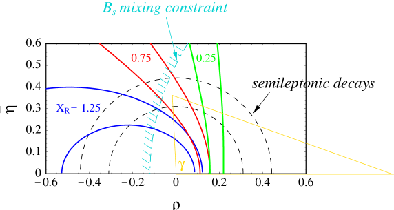
Figure 13: Allowed regions in the $(\bar{\rho},\bar{\eta})$ plane for fixed values of $X_{R}$, obtained by varying all theoretical parameters inside their respective ranges of uncertainty, as specified in the text. The sign of $\bar{\eta}$ is not determined.

Solving the equation for $R_{*}$ in (5.1) for $\cos\gamma$, and including the corrections of $O(\varepsilon_{a})$, we find

$$\cos\gamma=\delta_{\rm EW}-\frac{X_{R}+\frac{1}{2}\bar{\varepsilon}_{3/2}(X_{R}^{2}-1+\delta_{\rm EW}^{2})}{\cos\phi+\bar{\varepsilon}_{3/2}\delta_{\rm EW}}+\frac{\varepsilon_{a}\cos\eta\sin^{2}\!\gamma}{\cos\phi+\bar{\varepsilon}_{3/2}\delta_{\rm EW}}\,,$$ (95)

where we have set $\cos\phi=1$ in the numerator of the $O(\varepsilon_{a})$ term. Using the QCD factorization theorem one finds that $\varepsilon_{a}\cos\eta\approx-0.02$ in the heavy-quark limit $\!{}^{{\bf?}}$, and we assign a 100% uncertainty to this estimate. In evaluating the result (95) we scan the parameters in the ranges $0.15\leq\bar{\varepsilon}_{3/2}\leq 0.27$, $0.55\leq\delta_{\rm EW}\leq 0.73$, $-25^{\circ}\leq\phi\leq 25^{\circ}$, and $-0.04\leq\varepsilon_{a}\cos\eta\sin^{2}\!\gamma\leq 0$. Figure 13 shows the allowed regions in the $(\bar{\rho},\bar{\eta})$ plane for the representative values $X_{R}=0.25$, 0.75, and 1.25 (from right to left). We stress that with this method a useful constraint on the Wolfenstein parameters is obtained for any value of $X_{R}$.

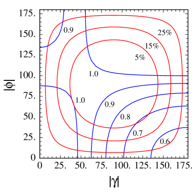
Figure 14: Contours of constant $R_{*}$ (“hyperbolas”) and constant $|\widetilde{A}|$ (“circles”) in the $(|\gamma|,|\phi|)$ plane. The sign of the asymmetry $\widetilde{A}$ determines the sign of the product $\sin\gamma\sin\phi$. The contours for $R_{*}$ refer to values from 0.6 to 1.0 in steps of 0.1, those for the asymmetry correspond to 5%, 15%, and 25%, as indicated.

Model-independent determination:
It is important that, once more precise data on $B^{\pm}\to\pi K$ decays will become available, it will be possible to test the prediction of a small strong phase $\phi$ experimentally. To this end, one must determine the CP asymmetry $\widetilde{A}$ defined in (90) in addition to the ratio $R_{*}$. From (5.1) it follows that for fixed values of $\bar{\varepsilon}_{3/2}$ and $\delta_{\rm EW}$ the quantities $R_{*}$ and $\widetilde{A}$ define contours in the $(\gamma,\phi)$ plane, whose intersections determine the two phases up to possible discrete ambiguities $\!{}^{{\bf?},{\bf?}}$. Figure 14 shows these contours for some representative values, assuming $\bar{\varepsilon}_{3/2}=0.21$, $\delta_{\rm EW}=0.64$, and $\varepsilon_{a}=0$. In practice, including the uncertainties in the values of these parameters changes the contour lines into contour bands. Typically, the spread of the bands induces an error in the determination of $\gamma$ of about $\!{}^{{\bf?}}$ $10^{\circ}$. In the most general case there are up to eight discrete solutions for the two phases, four of which are related to the other four by a sign change $(\gamma,\phi)\to(-\gamma,-\phi)$. However, for typical values of $R_{*}$ it turns out that often only four solutions exist, two of which are related to the other two by a sign change. The theoretical prediction that $\phi$ is small implies that solutions should exist where the contours intersect close to the lower portion in the plot. Other solutions with large $\phi$ are strongly disfavored. Note that according to (5.1) the sign of the CP asymmetry $\widetilde{A}$ fixes the relative sign between the two phases $\gamma$ and $\phi$. If we trust the theoretical prediction that $\phi$ is negative $\!{}^{{\bf?}}$, it follows that in most cases there remains only a unique solution for $\gamma$, i.e. the CP-violating phase $\gamma$ can be determined without any discrete ambiguity.

Consider, as an example, the hypothetical case where $R_{*}=0.8$ and $\widetilde{A}=-15\%$. Figure 14 then allows the four solutions where $(\gamma,\phi)\approx(\pm 82^{\circ},\mp 21^{\circ})$ or $(\pm 158^{\circ},\mp 78^{\circ})$. The second pair of solutions is strongly disfavored because of the large values of the strong phase $\phi$. From the first pair of solutions, the one with $\phi\approx-21^{\circ}$ is closest to our theoretical expectation that $\phi\approx-11^{\circ}$, hence leaving $\gamma\approx 82^{\circ}$ as the unique solution.

6 Sensitivity to New Physics

In the presence of New Physics the theoretical description of $B^{\pm}\to\pi K$ decays becomes more complicated. In particular, new CP-violating contributions to the decay amplitudes may be induced. A detailed analysis of such effects has been presented in $\!{}^{{\bf?}}$. A convenient and completely general parameterization of the two amplitudes in (5.1) is obtained by replacing

$$P\to P^{\prime}\,,\qquad\varepsilon_{a}\,e^{i\gamma}e^{i\eta}\to i\rho\,e^{i\phi_{\rho}}\,,\qquad\delta_{\rm EW}\to a\,e^{i\phi_{a}}+ib\,e^{i\phi_{b}}\,,$$ (96)

where $\rho$, $a$, $b$ are real hadronic parameters, and $\phi_{\rho}$, $\phi_{a}$, $\phi_{b}$ are strong phases. The terms $i\rho$ and $ib$ change sign under a CP transformation. New Physics effects parameterized by $P^{\prime}$ and $\rho$ are isospin conserving, while those described by $a$ and $b$ violate isospin symmetry. Note that the parameter $P^{\prime}$ cancels in all ratios of branching ratios and thus does not affect the quantities $R_{*}$ and $X_{R}$ as well as any CP asymmetry. Because the ratio $R_{*}$ in (89) would be 1 in the limit of isospin symmetry, it is particularly sensitive to isospin-violating New Physics contributions.

New Physics can affect the bound on $\gamma$ derived from (92) as well as the extraction of $\gamma$ using the strategies discussed above. We will discuss these two possibilities in turn.

6.1 Effects on the Bound on $\gamma$

The upper bound on $R_{*}^{-1}$ in (92) and the corresponding bound on $X_{R}$ shown in Fig. 11 are model-independent results valid in the Standard Model. Note that the extremal value of $R_{*}^{-1}$ is such that $|X_{R}|\leq(1+\delta_{\rm EW})$ irrespective of $\gamma$. A value of $|X_{R}|$ exceeding this bound would be a clear signal for New Physics $\!{}^{{\bf?},{\bf?},{\bf?}}$.

Consider first the case where New Physics may induce arbitrary CP-violating contributions to the $B\to\pi K$ decay amplitudes, while preserving isospin symmetry. Then the only change with respect to the Standard Model is that the parameter $\rho$ may no longer be as small as $O(\varepsilon_{a})$. Varying the strong phases $\phi$ and $\phi_{\rho}$ independently, and allowing for an arbitrarily large New Physics contribution to $\rho$, one can derive the bound $\!{}^{{\bf?}}$

$$|X_{R}|\leq\sqrt{1-2\delta_{\rm EW}\cos\gamma+\delta_{\rm EW}^{2}}\leq 1+\delta_{\rm EW}\,.$$ (97)

The extremal value is the same as in the Standard Model, i.e. isospin-conserving New Physics effects cannot lead to a value of $|X_{R}|$ exceeding $(1+\delta_{\rm EW})$. For intermediate values of $\gamma$ the Standard Model bound on $X_{R}$ is weakened; but even for large $\rho=O(1)$, corresponding to a significant New Physics contribution to the decay amplitudes, the effect is small.

If both isospin-violating and isospin-conserving New Physics contributions are present and involve new CP-violating phases, the analysis becomes more complicated. Still, it is possible to derive model-independent bounds on $X_{R}$. Allowing for arbitrary values of $\rho$ and all strong phases, one obtains $\!{}^{{\bf?}}$

$$|X_{R}| \leq \sqrt{(|a|+|\cos\gamma|)^{2}+(|b|+|\sin\gamma|)^{2}}$$ (98)

$$\leq 1+\sqrt{a^{2}+b^{2}}\leq\frac{2}{\bar{\varepsilon}_{3/2}}+X_{R}\,,$$

where the last inequality is relevant only in cases where $\sqrt{a^{2}+b^{2}}\gg 1$. The important point to note is that with isospin-violating New Physics contributions the value of $|X_{R}|$ can exceed the upper bound in the Standard Model by a potentially large amount. For instance, if $\sqrt{a^{2}+b^{2}}$ is twice as large as in the Standard Model, corresponding to a New Physics contribution to the decay amplitudes of only 10–15%, then $|X_{R}|$ could be as large as 2.6 as compared with the maximal value 1.8 allowed (for arbitrary $\gamma$) in the Standard Model. Also, in the most general case where $b$ and $\rho$ are non-zero, the maximal value $|X_{R}|$ can take is no longer restricted to occur at the endpoints $\gamma=0^{\circ}$ or $180^{\circ}$, which are disfavored by the global analysis of the unitarity triangle $\!{}^{{\bf?}}$. Rather, $|X_{R}|$ would take its maximal value if $|\tan\gamma|=|\rho|=|b/a|$.

The present experimental value of $X_{R}$ in (93) has too large an error to determine whether there is any deviation from the Standard Model. If $X_{R}$ turns out to be larger than 1 (i.e. at least one third of a standard deviation above its current central value), then an interpretation of this result in the Standard Model would require a large value $|\gamma|>91^{\circ}$ (see Fig. 11), which would be difficult to accommodate in view of the upper bound implied by the experimental constraint on $B_{s}$–$\bar{B}_{s}$ mixing, thus providing evidence for New Physics. If $X_{R}>1.3$, one could go a step further and conclude that the New Physics must necessarily violate isospin $\!{}^{{\bf?}}$.

6.2 Effects on the Determination of $\gamma$

A value of the observable $R_{*}$ violating the bound (92) would be an exciting hint for New Physics. However, even if a future precise measurement will give a value that is consistent with the Standard Model bound, $B^{\pm}\to\pi K$ decays provide an excellent testing ground for physics beyond the Standard Model. This is so because New Physics may cause a significant shift in the value of $\gamma$ extracted using the strategies discussed earlier, leading to inconsistencies when this value is compared with other determinations of $\gamma$.

A global fit of the unitarity triangle combining information from semi-leptonic $B$ decays, $B$–$\bar{B}$ mixing, CP violation in the kaon system, and mixing-induced CP violation in $B\to J/\psi\,K_{S}$ decays provides information on $\gamma$ which in a few years will determine its value within a rather narrow range $\!{}^{{\bf?}}$. Such an indirect determination could be complemented by direct measurements of $\gamma$ using, e.g., $B\to DK^{(*)}$ decays, or using the triangle relation $\gamma=180^{\circ}-\alpha-\beta$ combined with a measurement of $\alpha$. We will assume that a discrepancy of more than $25^{\circ}$ between the “true” $\gamma=\mbox{arg}(V_{ub}^{*})$ and the value $\gamma_{\pi K}$ extracted in $B^{\pm}\to\pi K$ decays will be observable after a few years of operation at the $B$ factories. This sets the benchmark for sensitivity to New Physics effects.

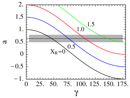
Figure 15: Contours of constant $X_{R}$ versus $\gamma$ and the parameter $a$, assuming $\gamma>0$. The horizontal band shows the value of $a$ in the Standard Model.

In order to illustrate how big an effect New Physics could have on the extracted value of $\gamma$, we consider the simplest case where there are no new CP-violating couplings. Then all New Physics contributions in (96) are parameterized by the single parameter $a_{\rm NP}\equiv a-\delta_{\rm EW}$. A more general discussion can be found in Ref. 127. We also assume for simplicity that the strong phase $\phi$ is small, as suggested by (94). In this case the difference between the value $\gamma_{\pi K}$ extracted from $B^{\pm}\to\pi K$ decays and the “true” value of $\gamma$ is to a good approximation given by

$$\cos\gamma_{\pi K}\simeq\cos\gamma-a_{\rm NP}\,.$$ (99)

In Fig. 15 we show contours of constant $X_{R}$ versus $\gamma$ and $a$, assuming without loss of generality that $\gamma>0$. Obviously, even a moderate New Physics contribution to the parameter $a$ can induce a large shift in $\gamma$. Note that the present central value of $X_{R}\approx 0.7$ is such that values of $a$ less than the Standard Model result $a\approx 0.64$ are disfavored, since they would require values of $\gamma$ exceeding $100^{\circ}$, in conflict with the global analysis of the unitarity triangle $\!{}^{{\bf?}}$.

6.3 Survey of New Physics models

In Ref. 127, we have explored how New Physics could affect purely hadronic FCNC transitions of the type $\bar{b}\to\bar{s}q\bar{q}$ focusing, in particular, on isospin violation. Unlike in the Standard Model, where isospin-violating effects in these processes are suppressed by electroweak gauge couplings or small CKM matrix elements, in many New Physics scenarios these effects are not parametrically suppressed relative to isospin-conserving FCNC processes. In the language of effective weak Hamiltonians this implies that the Wilson coefficients of QCD and electroweak penguin operators are of a similar magnitude. For a large class of New Physics models we found that the coefficients of the electroweak penguin operators are, in fact, due to “trojan” penguins, which are neither related to penguin diagrams nor of electroweak origin.

Specifically, we have considered: (a) models with tree-level FCNC couplings of the $Z$ boson, extended gauge models with an extra $Z^{\prime}$ boson, supersymmetric models with broken R-parity; (b) supersymmetric models with R-parity conservation; (c) two-Higgs-doublet models, and models with anomalous gauge-boson couplings. Some of these models have also been investigated in Refs. 125 and 126. In case (a), the electroweak penguin coefficients can be much larger than in the Standard Model because they are due to tree-level processes. In case (b), these coefficients can compete with the ones of the Standard Model because they arise from strong-interaction box diagrams, which scale relative to the Standard Model like $(\alpha_{s}/\alpha)(m_{W}^{2}/m_{\rm SUSY}^{2})$. In models (c), on the other hand, isospin-violating New Physics effects are not parametrically enhanced and are generally smaller than in the Standard Model.

Table 1: Maximal contributions to $a_{\rm NP}$ and shifts in $\gamma$ in extensions of the Standard Model. For the case of supersymmetric models with R-parity the first (second) row corresponds to maximal right-handed (left-handed) strange-bottom squark mixing. For the two-Higgs-doublet models we take $m_{H^{+}}>100$ GeV and $\tan\beta>1$.

Model $|a_{\rm NP}|$ $|\gamma_{\pi K}-\gamma|$ FCNC $Z$ exchange 2.0 $180^{\circ}$ extra $Z^{\prime}$ boson 14 $180^{\circ}$ SUSY without R-parity 14 $180^{\circ}$ SUSY with R-parity 0.4 $25^{\circ}$ 1.3 $180^{\circ}$ two-Higgs-doublet models 0.15 $10^{\circ}$ anomalous gauge-boson couplings 0.3 $20^{\circ}$

For each New Physics model we have explored which region of parameter space can be probed by the $B^{\pm}\to\pi K$ observables, and how big a departure from the Standard Model predictions one can expect under realistic circumstances, taking into account all constraints on the model parameters implied by other processes. Table 1 summarizes our estimates of the maximal isospin-violating contributions to the decay amplitudes, as parameterized by $|a_{\rm NP}|$. They are the potentially most important source of New Physics effects in $B^{\pm}\to\pi K$ decays. For comparison, we recall that in the Standard Model $a\approx 0.64$. Also shown are the corresponding maximal values of the difference $|\gamma_{\pi K}-\gamma|$. As noted above, in models with tree-level FCNC couplings New Physics effects can be dramatic, whereas in supersymmetric models with R-parity conservation isospin-violating loop effects can be competitive with the Standard Model. In the case of supersymmetric models with R-parity violation the bound (98) implies interesting limits on certain combinations of the trilinear couplings $\lambda_{ijk}^{\prime}$ and $\lambda_{ijk}^{\prime\prime}$, as discussed in Ref. 127.

7 Concluding Remarks

We have presented an introduction to recent developments in the theory and phenomenology of $B$ physics, focusing on heavy-quark symmetry, exclusive and inclusive weak decays of $B$ mesons, and rare $B$ decays that are sensitive to CP-violating weak phases of the Standard Model. The theoretical tools that allow us to perform quantitative calculations are various forms of heavy-quark expansions, i.e. expansions in logarithms and inverse powers of the large scale provided by the heavy-quark mass, $m_{b}\gg\Lambda_{\rm QCD}$.

Heavy-flavor physics is a rich and diverse area of current research, which is characterized by a fruitful interplay between theory and experiments. This has led to many significant discoveries and developments. $B$ physics has the potential to determine many important parameters of the electroweak theory and to test the Standard Model at low energies. At the same time, through the study of CP violation it provides a window to physics beyond the Standard Model. Indeed, there is a fair chance that such New Physics will first be seen at the $B$ factories, before it can be explored in future collider experiments at the Tevatron and the Large Hadron Collider.

Acknowledgements: It is a great pleasure to thank the Organizers of the Trieste Summer School in Particle Physics for the invitation to present these lectures and for providing a stimulating and relaxing atmosphere, which helped to initiate many physics discussions. In particular, I wish to express my gratitude to Gia Dvali, Antonio Masiero, Goran Senjanovic and Alexei Smirnov for their great hospitality and their many efforts to make my stay in Trieste a memorable one. Last but not least, I wish to thank the students of the school for their lively interest in these lectures.

References

References

- [1] E.V. Shuryak, Phys. Lett. B 93, 134 (1980); Nucl. Phys. B 198, 83 (1982).
-
[2]
J.E. Paschalis and G.J. Gounaris, Nucl. Phys. B 222, 473
(1983);
F.E. Close, G.J. Gounaris, and J.E. Paschalis, Phys. Lett. B 149, 209 (1984). - [3] S. Nussinov and W. Wetzel, Phys. Rev. D 36, 130 (1987).
- [4] M.B. Voloshin and M.A. Shifman, Yad. Fiz. 45, 463 (1987) [Sov. J. Nucl. Phys. 45, 292 (1987)].
- [5] M.B. Voloshin and M.A. Shifman, Yad. Fiz. 47, 801 (1988) [Sov. J. Nucl. Phys. 47, 511 (1988)].
- [6] N. Isgur and M.B. Wise, Phys. Lett. B 232, 113 (1989); 237, 527 (1990).
- [7] E. Eichten and F. Feinberg, Phys. Rev. D 23, 2724 (1981).
- [8] W.E. Caswell and G.P. Lepage, Phys. Lett. B 167, 437 (1986).
- [9] E. Eichten, in: Field Theory on the Lattice, edited by A. Billoire et al., Nucl. Phys. B (Proc. Suppl.) 4, 170 (1988).
- [10] G.P. Lepage and B.A. Thacker, in: Field Theory on the Lattice, edited by A. Billoire et al., Nucl. Phys. B (Proc. Suppl.) 4, 199 (1988).
- [11] H.D. Politzer and M.B. Wise, Phys. Lett. B 206, 681 (1988); 208, 504 (1988).
- [12] E. Eichten and B. Hill, Phys. Lett. B 234, 511 (1990); 243, 427 (1990).
- [13] B. Grinstein, Nucl. Phys. B 339, 253 (1990).
- [14] H. Georgi, Phys. Lett. B 240, 447 (1990).
- [15] A.F. Falk, H. Georgi, B. Grinstein, and M.B. Wise, Nucl. Phys. B 343, 1 (1990).
- [16] A.F. Falk, B. Grinstein, and M.E. Luke, Nucl. Phys. B 357, 185 (1991).
- [17] T. Mannel, W. Roberts, and Z. Ryzak, Nucl. Phys. B 368, 204 (1992).
- [18] M. Neubert, Phys. Rep. 245, 259 (1994); Int. J. Mod. Phys. A 11, 4173 (1996).
- [19] H. Georgi, in: Perspectives in the Standard Model, Proceedings of the Theoretical Advanced Study Institute in Elementary Particle Physics (TASI-91), Boulder, Colorado, 1991, edited by R.K. Ellis, C.T. Hill, and J.D. Lykken (World Scientific, Singapore, 1992), p. 589.
- [20] B. Grinstein, in: High Energy Phenomenology, Proceedings of the Workshop on High Energy Phenomenology, Mexico City, Mexico, 1991, edited by M.A. Péres and R. Huerta (World Scientific, Singapore, 1992), p. 161.
- [21] N. Isgur and M.B. Wise, in: Heavy Flavours, edited by A.J. Buras and M. Lindner (World Scientific, Singapore, 1992), p. 234.
- [22] T. Mannel, in: QCD-20 Years Later, Proceedings of the Workshop on QCD, Aachen, Germany, 1992, edited by P.M. Zerwas and H.A. Kastrup (World Scientific, Singapore, 1993), p. 634; Chinese J. Phys. 31, 1 (1993).
- [23] M. Shifman, in: QCD and Beyond, Proceedings of the Theoretical Advanced Study Institute in Elementary Particle Physics, Boulder, Colorado, June 1995, edited by D.E. Soper (World Scientific, Singapore, 1996), p. 409.
- [24] A. Falk, in: The Strong Interaction, from Hadrons to Partons, Proceedings of the 24th SLAC Summer Institute on Particle Physics, Stanford, California, August 1996, edited by J. Chan et al. (SLAC Report No. SLAC-R-508), p. 43.
- [25] D.J. Gross and F. Wilczek, Phys. Rev. Lett. 30, 1343 (1973).
- [26] H.D. Politzer, Phys. Rev. Lett. 30, 1346 (1973).
- [27] M.A. Shifman, A.I. Vainshtein, and V.I. Zakharov, Nucl. Phys. B 120, 316 (1977).
- [28] E. Witten, Nucl. Phys. B 122, 109 (1977).
- [29] J. Polchinski, Nucl. Phys. B 231, 269 (1984).
- [30] K. Wilson, Phys. Rev. 179, 1499 (1969); D 3, 1818 (1971).
- [31] W. Zimmermann, Ann. Phys. 77, 536 and 570 (1973).
- [32] G. Altarelli and L. Maiani, Phys. Lett. B 52, 351 (1974).
- [33] M.K. Gaillard and B.W. Lee, Phys. Rev. Lett. 33, 108 (1974).
- [34] F.J. Gilman and M.B. Wise, Phys. Rev. D 27, 1128 (1983).
- [35] J. Soto and R. Tzani, Phys. Lett. B 297, 358 (1992).
- [36] A.F. Falk, M. Neubert, and M.E. Luke, Nucl. Phys. B 388, 363 (1992).
- [37] R. Tarrach, Nucl. Phys. B 183, 384 (1981).
- [38] M.A. Shifman, A.I. Vainshtein, and V.I. Zakharov, Nucl. Phys. B 147, 385 and 448 (1979).
- [39] G. ’t Hooft, in: The Whys of Subnuclear Physics, Proceedings of the 15th International School on Subnuclear Physics, Erice, Sicily, 1977, edited by A. Zichichi (Plenum Press, New York, 1979), p. 943.
- [40] B. Lautrup, Phys. Lett. B 69, 109 (1977).
- [41] G. Parisi, Phys. Lett. B 76, 65 (1978); Nucl. Phys. B 150, 163 (1979).
- [42] F. David, Nucl. Phys. B 234, 237 (1984); 263, 637 (1986).
- [43] A.H. Mueller, Nucl. Phys. B 250, 327 (1985).
-
[44]
V.I. Zakharov, Nucl. Phys. B 385, 452 (1992);
M. Beneke and V.I. Zakharov, Phys. Rev. Lett. 69, 2472 (1992). - [45] M. Beneke, Phys. Lett. B 307, 154 (1993); Nucl. Phys. B 405, 424 (1993).
- [46] D. Broadhurst, Z. Phys. C 58, 339 (1993).
- [47] A.H. Mueller, in: QCD – 20 Years Later, edited by P.M. Zerwas and H.A. Kastrup (World Scientific, Singapore, 1993), p. 162; Phys. Lett. B 308, 355 (1993).
- [48] M. Beneke and V.M. Braun, Nucl. Phys. B 426, 301 (1994).
- [49] I.I. Bigi, M.A. Shifman, N.G. Uraltsev, and A.I. Vainshtein, Phys. Rev. D 50, 2234 (1994).
- [50] M. Neubert and C.T. Sachrajda, Nucl. Phys. B 438, 235 (1995).
- [51] M. Beneke, V.M. Braun, and V.I. Zakharov, Phys. Rev. Lett. 73, 3058 (1994).
- [52] M. Luke, A.V. Manohar, and M.J. Savage, Phys. Rev. D 51, 4924 (1995).
- [53] N. Isgur and M.B. Wise, Phys. Rev. Lett. 66, 1130 (1991).
- [54] U. Aglietti, Phys. Lett. B 281, 341 (1992); Int. J. Mod. Phys. A 10, 801 (1995).
- [55] A.F. Falk, Nucl. Phys. B 378, 79 (1992).
- [56] A.F. Falk and M. Neubert, Phys. Rev. D 47, 2965 and 2982 (1993).
- [57] V. Eletsky and E. Shuryak, Phys. Lett. B 276, 191 (1992).
- [58] P. Ball and V.M. Braun, Phys. Rev. D 49, 2472 (1994).
- [59] M. Neubert, Phys. Lett. B 389, 727 (1996); 322, 419 (1994).
- [60] V. Giménez, G. Martinelli, and C.T. Sachrajda, Nucl. Phys. B 486, 227 (1997).
- [61] I. Bigi, M. Shifman, N.G. Uraltsev, and A. Vainshtein, Phys. Rev. D 52, 196 (1995).
- [62] M. Gremm, A. Kapustin, Z. Ligeti, and M.B. Wise, Phys. Rev. Lett. 77, 20 (1996).
- [63] A.F. Falk, M. Luke, and M.J. Savage, Phys. Rev. D 53, 6316 (1996).
- [64] V. Chernyak, Nucl. Phys. B 457, 96 (1995); Phys. Lett. B 387, 173 (1996).
- [65] D.S. Hwang, C.S. Kim, and W. Namgung, Phys. Rev. D 54, 5620 (1996); Phys. Lett. B 406, 117 (1997).
- [66] F. De Fazio, Mod. Phys. Lett. A 11, 2693 (1996).
- [67] M. Neubert and V. Rieckert, Nucl. Phys. B 382, 97 (1992).
- [68] M. Neubert, Phys. Lett. B 264, 455 (1991).
- [69] M.E. Luke, Phys. Lett. B 252, 447 (1990).
- [70] M. Ademollo and R. Gatto, Phys. Rev. Lett. 13, 264 (1964).
- [71] M. Neubert, Nucl. Phys. B 416, 786 (1994).
- [72] P. Cho and B. Grinstein, Phys. Lett. B 285, 153 (1992).
-
[73]
C.G. Boyd, B. Grinstein, and R.F. Lebed, Phys. Lett. B 353,
306 (1995); Nucl. Phys. B 461, 493 (1996); Phys. Rev. D
56, 6895 (1997);
C.G. Boyd and R.F. Lebed, Nucl. Phys. B 485, 275 (1997). -
[74]
I. Caprini and M. Neubert, Phys. Lett. B 380, 376 (1996);
I. Caprini, L. Lellouch, and M. Neubert, Nucl. Phys. B 530, 153 (1998). - [75] CLEO Collaboration (B. Barish et al.), Phys. Rev. D 51, 1041 (1995).
- [76] P.S. Drell, in: Proceedings of the 18th International Symposium on Lepton-Photon Interactions, Hamburg, Germany, July 1997, edited by A. De Roeck and A. Wagner (World Scientific, Singapore, 1998), p. 347.
- [77] M. Neubert, Nucl. Phys. B 371, 149 (1992).
-
[78]
S.J. Brodsky, G.P. Lepage, and P.B. Mackenzie, Phys. Rev. D 28, 228 (1983);
G.P. Lepage and P.B. Mackenzie, Phys. Rev. D 48, 2250 (1993). - [79] M. Neubert, Phys. Lett. B 341, 367 (1995).
- [80] X. Ji and M.J. Musolf, Phys. Lett. B 257, 409 (1991).
- [81] D.J. Broadhurst and A.G. Grozin, Phys. Lett. B 267, 105 (1991).
- [82] A.F. Falk and B. Grinstein, Phys. Lett. B 247, 406 (1990).
- [83] M. Neubert, Phys. Rev. D 46, 2212 (1992).
- [84] M. Neubert, Phys. Rev. D 51, 5924 (1995).
- [85] A. Czarnecki, Phys. Rev. Lett. 76, 4124 (1996).
- [86] T. Mannel, Phys. Rev. D 50, 428 (1994).
- [87] M. Shifman, N.G. Uraltsev, and A. Vainshtein, Phys. Rev. D 51, 2217 (1995).
- [88] M. Neubert, Phys. Lett. B 338, 84 (1994).
-
[89]
M. Neubert, Phys. Rev. D 46, 3914 (1992);
Z. Ligeti, Y. Nir, and M. Neubert, Phys. Rev. D 49, 1302 (1994). - [90] CLEO Collaboration (J.E. Duboscq et al.), Phys. Rev. Lett. 76, 3898 (1996).
- [91] M. Neubert, Phys. Rev. D 46, 1076 (1992).
- [92] E. Bagan, P.Ball, V.M. Braun, and H.G. Dosch, Phys. Lett. B 278, 457 (1992).
- [93] F.E. Close and A. Wambach, Phys. Lett. B 348, 207 (1995).
- [94] CLEO Collaboration (T. Bergfeld et al.), Preprint CLEO CONF 96-3 (1996); CLEO Collaboration (J. Bartelt et al.), Phys. Rev. Lett. 82, 3746 (1999).
- [95] ALEPH Collaboration (D. Buskulic et al.), Phys. Lett. B 395, 373 (1997).
- [96] J. Chay, H. Georgi, and B. Grinstein, Phys. Lett. B 247, 399 (1990).
-
[97]
I.I. Bigi, N.G. Uraltsev, and A.I. Vainshtein, Phys. Lett. B 293, 430 (1992) [E: 297, 477 (1993)];
I.I. Bigi, M.A. Shifman, N.G. Uraltsev, and A.I. Vainshtein, Phys. Rev. Lett. 71, 496 (1993);
I.I. Bigi et al., in: Proceedings of the Annual Meeting of the Division of Particles and Fields of the APS, Batavia, Illinois, 1992, edited by C. Albright et al. (World Scientific, Singapore, 1993), p. 610. - [98] B. Blok, L. Koyrakh, M.A. Shifman, and A.I. Vainshtein, Phys. Rev. D 49, 3356 (1994) [E: 50, 3572 (1994)].
- [99] A.V. Manohar and M.B. Wise, Phys. Rev. D 49, 1310 (1994).
-
[100]
M. Luke and M.J. Savage, Phys. Lett. B 321, 88 (1994);
A.F. Falk, M. Luke, and M.J. Savage, Phys. Rev. D 49, 3367 (1994). - [101] T. Mannel, Nucl. Phys. B 413, 396 (1994).
- [102] A.F. Falk, Z. Ligeti, M. Neubert, and Y. Nir, Phys. Lett. B 326, 145 (1994).
- [103] M. Neubert, Phys. Rev. D 49, 3392 and 4623 (1994).
- [104] I.I. Bigi, M.A. Shifman, N.G. Uraltsev, and A.I. Vainshtein, Int. J. Mod. Phys. A 9, 2467 (1994).
- [105] T. Mannel and M. Neubert, Phys. Rev. D 50, 2037 (1994).
- [106] E.C. Poggio, H.R. Quinn, and S. Weinberg, Phys. Rev. D 13, 1958 (1976).
- [107] M. Girone and M. Neubert, Phys. Rev. Lett. 76, 3061 (1996).
- [108] F.G. Gilman and M.B. Wise, Phys. Rev. D 20, 2392 (1979).
- [109] G. Altarelli, G. Curci, G. Martinelli, and S. Petrarca, Phys. Lett. B 99, 141 (1981); Nucl. Phys. B 187, 461 (1981).
- [110] A.J. Buras and P.H. Weisz, Nucl. Phys. B 333, 66 (1990).
- [111] G. Altarelli et al., Nucl. Phys. B 208, 365 (1982).
- [112] C.H. Jin, W.F. Palmer, and E.A. Paschos, Phys. Lett. B 329, 364 (1994); A. Bareiss and E.A. Paschos, Nucl. Phys. B 327, 353 (1989).
- [113] Y. Nir, Phys. Lett. B 221, 184 (1989).
- [114] A. Czarnecki and K. Melnikov, Nucl. Phys. B 505, 65 (1997); Phys. Rev. Lett. 78, 3630 (1997); Phys. Rev. D 59, 014036 (1999).
- [115] For a review, see: The BaBar Physics Book, P.F. Harison and H.R. Quinn eds., SLAC Report No. SLAC-R-504 (1998).
-
[116]
A documentation of this measurement can be found at
http://www-cdf.fnal.gov/physics/new/bottom/cdf4855. - [117] KTeV Collaboration (A. Alavi-Harati et al.), Phys. Rev. Lett. 83, 22 (1999).
-
[118]
A documentation of this measurement can be found at
http://www.cern.ch/NA48. - [119] M. Neubert and J.R. Rosner, Phys. Lett. B 441, 403 (1998).
- [120] M. Neubert and J.R. Rosner, Phys. Rev. Lett. 81, 5076 (1998).
- [121] M. Neubert, J. High Energy Phys. 02, 014 (1999).
- [122] M. Beneke, G. Buchalla, M. Neubert, and C.T. Sachrajda, Phys. Rev. Lett. 83, 1914 (1999).
- [123] M. Neubert and B. Stech, in: Heavy Flavours (2nd Edition), edited by A.J. Buras and M. Lindner (World Scientific, Singapore, 1998), p. 294.
-
[124]
R. Fleischer and J. Matias, Preprint CERN-TH-99-164
[hep-ph/9906274]. - [125] D. Choudhury, B. Dutta, and A. Kundu, Phys. Lett. B 456, 185 (1999).
- [126] X.-G. He, C.-L. Hsueh, and J.-Q. Shi, Phys. Rev. Lett. 84, 18 (2000).
- [127] Y. Grossman, M. Neubert, and A.L. Kagan, J. High Energy Phys. 10, 029 (1999).
- [128] For a review, see: G. Buchalla, A.J. Buras, and M.E. Lautenbacher, Rev. Mod. Phys. 68, 1125 (1996).
- [129] A.S. Dighe, M. Gronau, and J.L. Rosner, Phys. Rev. Lett. 79, 4333 (1997).
- [130] N.G. Deshpande and X.-G. He, Phys. Rev. Lett. 74, 26 (1995) [E: 74, 4099 (1995)].
-
[131]
B. Blok, M. Gronau, and J.L. Rosner, Phys. Rev. Lett. 78,
3999 (1997);
M. Gronau and J.L. Rosner, Phys. Rev. D 58, 113005 (1998). - [132] A.J. Buras, R. Fleischer, and T. Mannel, Nucl. Phys. B 533, 3 (1998).
-
[133]
J.M. Gérard and J. Weyers, Eur. Phys. J. C 7, 1 (1999);
D. Delepine, J.M. Gérard, J. Pestieau, and J. Weyers, Phys. Lett. B 429, 106 (1998). - [134] M. Neubert, Phys. Lett. B 424, 152 (1998).
- [135] A.F. Falk, A.L. Kagan, Y. Nir, and A.A. Petrov, Phys. Rev. D 57, 4290 (1998).
- [136] D. Atwood and A. Soni, Phys. Rev. D 58, 036005 (1998).
- [137] M. Beneke, G. Buchalla, M. Neubert, and C.T. Sachrajda, in preparation.
-
[138]
R. Poling, Rapporteur’s talk presented at the 19th International
Symposium on Lepton and Photon Interactions at High Energies,
Stanford, California, 9–14 August 1999;
CLEO Collaboration, Conference contributions CLEO CONF 99-14 and CLEO CONF 99-16. - [139] R. Fleischer, Phys. Lett. B 365, 399 (1996).
- [140] M. Gronau, J.L. Rosner, and D. London, Phys. Rev. Lett. 73, 21 (1994).