Compactification, Geometry and Duality: $N=2$.

Abstract

We review the geometry of the moduli space of $N=2$ theories in four dimensions from the point of view of superstring compactification. The cases of a type IIA or type IIB string compactified on a Calabi–Yau threefold and the heterotic string compactified on K3$\times T^{2}$ are each considered in detail. We pay specific attention to the differences between $N=2$ theories and $N>2$ theories. The moduli spaces of vector multiplets and the moduli spaces of hypermultiplets are reviewed. In the case of hypermultiplets this review is limited by the poor state of our current understanding. Some peculiarities such as “mixed instantons” and the non-existence of a universal hypermultiplet are discussed.

1 Introduction

One of the most basic properties one may study about a class of string compactifications is its moduli space of vacua. If the class is suitably chosen one may find this a challenging subject which probes deeply into our understanding of string theory. In four dimensions it is the $N=2$ cases which provide the “Goldilocks” theories to study. As we will see, $N=4$ supersymmetry is too constraining and determines the moduli space exactly, leaving no room for interesting corrections from quantum effects. $N=1$ supersymmetry is highly unconstrained leaving the possibility that our supposed moduli acquire mass ruining the moduli space completely. $N=2$ however is just right — quantum effects are not potent enough to kill the moduli but they can affect the structure of the moduli space. (It is therefore a pity that the real world does not have $N=2$ supersymmetry — such a theory is necessarily non-chiral.)

The subject of $N=2$ compactifications is enormous and we will present here only a rather biased set of highlights. These lectures will be sometimes closely-related to a set of lectures I gave at TASI 3 years ago [1]. Having said that, the focus of these lectures differs from the former and the set of topics covered is not identical. I will however often refer to [1] for details of certain subjects.

Related to the problem of finding the moduli space of a class of theories is the following problem in string duality. Consider these four possibilities for obtaining an $N=2$ theory in four dimensions:

1. A type IIA string compactified on a Calabi–Yau threefold $X$.

2. A type IIB string compactified on a Calabi–Yau threefold $Y$.

3. An $E_{8}\times E_{8}$ heterotic string compactified on K3$\times T^{2}$.

4. A $\operatorname{Spin}(32)/{\mathbb{Z}}_{2}$ heterotic string compactified on K3$\times T^{2}$.

Can we find cases where the resulting 4 dimensional physics is identical for two or more of these possibilities and, if so, how do we match the moduli of these theories to each other? This is a story that began with [2, 3] some time ago but many details are poorly-understood to this day. One might suppose that knowing the moduli space of each theory listed above is a prerequisite for solving this problem but actually it is often useful, as we will see, to consider this duality problem at the same time as the moduli space problem. Note that there are other possibilities for producing $N=2$ theories in four dimensions such as the type I open string on K3$\times T^{2}$. We will stick with the four listed above in these lectures as they are quite sufficient for our purposes.

As will be discussed shortly this problem breaks up into two pieces. One factor of the moduli space consists of the vector multiplet moduli space and the other factor consists of the hypermultiplet moduli space. By most criteria the moduli space of vector multiplets is well-understood today. This complex Kähler space can be modeled exactly in terms of the deformation space of a Calabi–Yau threefold. We will therefore be able to review this subject fairly extensively.

In contrast the hypermultiplet moduli space remains a subject of research very much “in progress”. We will only be able to discuss in detail the classical boundaries of these moduli spaces. The interior of these spaces may offer considerable insight into string theory but we will only be able to cover some tantalizing hints of such possibilities.

These lectures divide naturally into three sections. In section 2 we discuss generalities about moduli spaces of various numbers of supersymmetries in various numbers of dimensions. Although these lectures are intended to focus on the case of $N=2$ in four dimensions, there are highly relevant observations that can be made by considering other possibilities. Of particular note in this section is the rigid structure which emerges with more supersymmetry than the case in question.

The heart of these lectures then consists of a discussion of the vector multiplet moduli space in section 3 and then the hypermultiplet moduli space in section 4. It is perhaps worth mentioning again that these lectures do not do justice to this vast subject and should be viewed as a biased account. Topic such as open strings, D-branes and M-theory have been neglected only because of the author’s groundless prejudices.

The paragraphs starting with a “✄” are technical and can be skipped if the reader does not wish to be embroiled in subtleties.

2 General Structure

2.1 Holonomy

We begin this section with a well-known derivation of key properties of moduli spaces based on $R$-symmetries and holonomy arguments. We should warn the more mathematically-inclined reader that we shall not endeavour to make completely watertight rigorous statements in the following. There may be a few pathological special cases which circumvent some of our (possibly implicit) assumptions.

Suppose we are given a vector bundle, $V$, with a connection. We may define the “holonomy”, $\operatorname{Hol}(V)$, of this bundle as the group generated by parallel transport around loops in the base with respect to this connection. (A choice of basepoint is unimportant.) We may also define the restricted holonomy group $\operatorname{Hol}^{0}(V)$ to be generated by contractable loops.

This notion can be very useful when applied to supersymmetric field theories as noted in [4]. First let us consider the moduli space of a given class of theories. We will consider the moduli space as the base space of a bundle. Note that the moduli space of theories, ${\Scr M}$, is equipped with a natural metric — that of the sigma-model. The tangent directions in the moduli space are given by the massless scalar fields with completely flat potentials. These massless fields may thus be given vacuum expectation values leading to a deformation of the theory. Let us denote these moduli fields $\phi^{i}$, $i=1,\ldots,\dim({\Scr M})$. The low-energy effective action in the uncompactified space-time is then given by

$$\int d^{d}x\,\sqrt{g}G_{ij}\partial^{\mu}\phi^{i}\partial_{\mu}\phi^{j}+\ldots$$ (1)

where $G_{ij}$ is our desired metric on ${\Scr M}$. We therefore have a natural torsion-free connection on the tangent bundle of ${\Scr M}$ given by the Levi-Civita connection with respect to this metric.

Now consider the supersymmetry generators given by spinors $Q_{A}$, $A=1,\ldots,N$, where as usual $N$ denotes the number of supersymmetries (we suppress the spinor index). These objects are representations of $\operatorname{Spin}(1,d-1)$ and are

• Real if $d=1,2,3\mod 8$

• Complex if $d=0,4\mod 8$

• Quaternionic (or symplectic Majorana) if $d=5,6,7\mod 8$.

The bundle of supersymmetry generators over ${\Scr M}$ will also have a natural connection related to that on the tangent bundle. The key relation in supersymmetry is the equation

$$\gamma_{\alpha\beta}^{\mu}\{\overline{Q}_{\bar{A}}^{\alpha},Q_{B}^{\beta}\}=\delta_{\bar{A}B}P^{\mu},$$ (2)

where $\gamma$ are the usual gamma matrices, $P$ is translation and the bars in this equation are to be interpreted according to whether the spinors are real, complex or quaternionic. Because parallel transport must preserve $\delta_{\bar{A}B}$ in (2) we see immediately that under holonomy $Q_{A}$ must transform as a fundamental representation of

• $\operatorname{SO}(N)$ if $d=1,2,3\mod 8$

• $\operatorname{U{}}(N)$ if $d=0,4\mod 8$

• $\operatorname{Sp}(N)$ if $d=5,6,7\mod 8$,

if the loop around which we transport is contractable. These groups are the “$R$-symmetries” of the supersymmetric field theories and give $\operatorname{Hol}^{0}$ of this bundle. We also note that in $4M+2$ dimensions, for integer $M$, the supersymmetries are chiral. This means that we consider left and right supersymmetries separately as we will illustrate in some examples below.

The massless scalar fields live in supermultiplets. Within each supermultiplet the set of scalar fields will form a particular (possibly trivial) representation of the $R$-symmetry. We refer to [5] for a detailed account of this. Occasionally the supermultiplet contains only one scalar component and this then transforms trivially under $R$. So long as this is not the case the holonomy of our tangent bundle is related to the $R$-symmetry.

We may be more precise than this. As we go around a loop in ${\Scr M}$ the scalars within every given supermultiplet will be mixed simultaneously by the $R$-symmetry. The supermultiplets themselves may also be mixed as a whole into each other by holonomy. This implies that, so long as the scalars transform nontrivially under $R$, the holonomy of the tangent bundle is factorized with the $R$-symmetry forming one factor. It is important to note however that we may not mix a scalar from one supermultiplet freely with any scalar from another supermultiplet in a way that violates this factorization. This is incompatible with the detailed supersymmetry transformation laws (as the reader might verify if they are unconvinced).

Note in particular that the scalars within two different types of supermultiplets can never mix under holonomy. This is a useful observation given the following due to De Rham (see, for example, [6])

Theorem 1

If a Riemannian manifold is complete, simply connected and if the holonomy of its tangent bundle with respect to the Levi-Civita connection is reducible, then this manifold is a product metrically.

Thus if ${\Scr M}$ is simply-connected we see that ${\Scr M}$ factorizes exactly into parts labelled by the type of supermultiplet containing the massless scalars. If ${\Scr M}$ is not simply-connected we may pass to the universal cover and use this theorem again. The general statement is therefore that the moduli space factorizes up to the quotient of a discrete group acting on the product.

• Actually we should treat the word “complete” in the above theorem with a little more care. There are nasty points at finite distance in the moduli space where the manifold structure breaks down. These points also lead to a breakdown in the factorization of the moduli space. These extremal transitions will be studied more in section 4.2. We should only say that the moduli space factorizes locally away from such points.

We may now analyze the structure of each factor of ${\Scr M}$ from the Berger-Simons theorem (for an account of this we refer again to [6]) which states that the manifold must appear as a row in the following list:

$$\begin{array}[]{c|c}\operatorname{Hol}^{0}&\dim({\Scr M})\\ \hline\cr\operatorname{SO}(n)&n\\ \operatorname{U{}}(n)&2n\\ \operatorname{SU}(n)&2n\\ \operatorname{Sp}(1).\operatorname{Sp}(n)&4n\\ \operatorname{Sp}(n)&4n\\ \operatorname{Spin}(7)&8\\ G_{2}&7\end{array}$$ (3)

or be a “symmetric space” (which we will define shortly). Note that the following names are given to some of these holonomies:

• Kähler if $\operatorname{Hol}\subset\operatorname{U{}}(n)$,

• Ricci-flat Kähler if $\operatorname{Hol}\subset\operatorname{SU}(n)$,

• Quaternionic Kähler if $\operatorname{Hol}\subset\operatorname{Sp}(1).\operatorname{Sp}(n)$,

• Hyperkähler if $\operatorname{Hol}\subset\operatorname{Sp}(n)$.

	Manifold	Real Dimension
A I	$\operatorname{SL}(n,{\mathbb{R}})/\operatorname{SO}(n)$	${\textstyle\frac{1}{2}}(n-1)(n+2)$
A II	$\operatorname{SU}^{*}(2n)/\operatorname{Sp}(n)$	$(n-1)(2n+1)$
A III	$\operatorname{SU}(p,q)/\mathrm{S}(\operatorname{U{}}(p)\times\operatorname{U{}}(q))$	$2pq$
BD I	$\operatorname{SO}_{0}(p,q)/(\operatorname{SO}(p)\times\operatorname{SO}(q))$	$pq$
D III	$\operatorname{SO}^{*}(2n)/\operatorname{U{}}(n)$	$n(n-1)$
C I	$\operatorname{Sp}(n,{\mathbb{R}})/\operatorname{U{}}(n)$	$n(n+1)$
C II	$\operatorname{Sp}(p,q)/(\operatorname{Sp}(p)\times\operatorname{Sp}(q))$	$4pq$
E I	$E_{6(6)}/\operatorname{Sp}(4)$	42
E II	$E_{6(2)}/(\operatorname{SU}(6)\times\operatorname{SU}(2))$	40
E III	$E_{6(-14)}/(\operatorname{SO}(10)\times\operatorname{U{}}(1))$	32
E IV	$E_{6(-26)}/F_{4}$	26
E V	$E_{7(7)}/\operatorname{SU}(8)$	70
E VI	$E_{7(-5)}/(\operatorname{SO}(12)\times\operatorname{SU}(2))$	64
E VII	$E_{7(-25)}/(E_{6}\times\operatorname{U{}}(1))$	54
E VIII	$E_{8(8)}/\operatorname{SO}(16)$	128
E IX	$E_{8(-24)}/(E_{7}\times\operatorname{SU}(2))$	112
F I	$F_{4(4)}/(\operatorname{Sp}(3)\times\operatorname{SU}(2))$	28
F II	$F_{4(-20)}/\operatorname{SO}(9)$	16
G I	$G_{2(2)}/(\operatorname{SU}(2)\times\operatorname{SU}(2))$	8

Table 1: Symmetric Spaces

A symmetric space is a Riemannian manifold which admits a “parity” ${\mathbb{Z}}_{2}$-symmetry about every point. This parity symmetry acts as $-1$ in every direction on the tangent space. All symmetric spaces are of the form $G/H$ for groups $G$ and $H$, where the holonomy is given by $H$. They have been classified by E. Cartan and we list all the noncompact forms in table 1. The noncompact forms are the ones relevant to moduli spaces.

A key point to note here is that the symmetric spaces are rigid — they have no deformations of the metric which would preserve the holonomy. The same is not true for the non-symmetric spaces listed in (3). Thus if the holonomy is of a type which forces a symmetric space as the only possibility we will refer to this as a rigid case.

Let us consider a few examples.

• $N=(1,1)$ in 6 dimensions (i.e., one left-moving supersymmetry and one right-moving supersymmetry). This implies that the $R$-symmetry is $\operatorname{Sp}(1)\times\operatorname{Sp}(1)=\operatorname{SO}(4)$ (up to irrelevant discrete groups). Analysis of the supermultiplets shows that matter supermultiplets have 4 scalars transforming as a 4 of $\operatorname{SO}(4)$. If we only had one such supermultiplet we could say nothing about the moduli space as a generic Riemannian manifold of 4 dimensions has holonomy $\operatorname{SO}(4)$. If we have a generic number, $n$, of supermultiplets and assuming the moduli space doesn’t factorize unnaturally then a quick look at the list above shows that the only possibility is the symmetric space. $\operatorname{SO}_{0}(4,n)/(\operatorname{SO}(4)\times\operatorname{SO}(n))$. Thus this case is rigid. The gravity supermultiplet has a single scalar giving an additional factor of ${\mathbb{R}}$ to the moduli space.

• $N=(2,0)$ in 6 dimensions. This implies that the $R$-symmetry is $\operatorname{Sp}(2)=\operatorname{SO}(5)$ (up to irrelevant discrete groups). Analysis of the supermultiplets shows that matter supermultiplets have 5 scalars transforming as a 5 of $\operatorname{SO}(5)$. If we have a generic number, $n$, of supermultiplets and assuming the moduli space doesn’t factorize unnaturally then the list above shows that the only possibility is the symmetric space $\operatorname{SO}_{0}(5,n)/(\operatorname{SO}(5)\times\operatorname{SO}(n))$. Thus this case is rigid. There are no further moduli.

• $N=4$ in 4 dimensions. This implies that the $R$-symmetry is $\operatorname{U{}}(4)=\operatorname{SO}(6)\times\operatorname{U{}}(1)$ (up to irrelevant discrete groups). Analysis of the supermultiplets shows that matter supermultiplets have 6 scalars transforming as a 6 of $\operatorname{SO}(6)$. If we have a generic number, $n$, of supermultiplets and assuming the moduli space doesn’t factorize unnaturally then the only possibility for this factor is the symmetric space $\operatorname{SO}_{0}(6,n)/(\operatorname{SO}(6)\times\operatorname{SO}(n))$. Thus this case is rigid. The gravity multiplet contains a complex scalar transforming under the $\operatorname{U{}}(1)$ factor of the holonomy. By holonomy arguments this contributes a complex Kähler factor to the moduli space. Closer analysis of this supergravity shows that this factor is actually $\operatorname{SL}(2,{\mathbb{R}})/\operatorname{U{}}(1)$.

This last example demonstrates an important point. Analysis of the $R$-symmetry may be sufficient to imply that we have a rigid moduli space but sometimes the moduli space is rigid even when the holonomy may imply otherwise. A more detailed analysis of the supergravity action is required in some cases to show that we indeed have a symmetric space. The rule of thumb is as follows: If we have maximal (32 supercharges, e.g. $N=8$ in four dimensions) or half-maximal (16 supercharges, e.g. $N=4$ in four dimensions) supersymmetry then, and usually only then, is the moduli space rigid. Note that there are a few strange examples such as [3] where the moduli space is rigid even when there are fewer than 16 supercharges.

2.2 U-Duality

In this section we will focus on global properties of the rigid moduli spaces. The analysis of the moduli spaces so far is not quite complete. The problem is that the moduli space need not be a manifold. There may be singular points corresponding to the theories with special properties. In the rigid case however the fact that the moduli space is symmetric wherever it is not singular is a very powerful constraint.

Let us suppose first that we have an orbifold point. That is a region in the moduli space which looks locally like a manifold divided by a discrete group fixing some point $x$. Away from the fixed point set the moduli space is symmetric and thus “homogeneous”. That is, there exist a transitive set of translation symmetries. Assuming geodesic completeness of the moduli space, these translations may be used to extend the local orbifold property to a global one. That is, the moduli space is globally of the form of a manifold divided by a discrete group [7].

This homogeneous structure of the moduli space may also be used to rule out other possibilities of singularities which occur at finite distance. Consider beginning at a smooth point in moduli space and approaching a singularity. The homogeneous structure implies that nothing about the local structure of the moduli space may change as you approach the singularity — everything happens suddenly as you hit the singularity. This rules out every other type of “reasonable” singularity that one may try to put in the moduli space. To be completely rigorous would require us to make precise technical definitions about the allowed geometry of the moduli space. Instead we shall just assert here that any type of singularity at finite distance that one might think of (such as a conifold) would ruin the homogeneous nature of the moduli space and so is not allowed in the rigid case.

We therefore arrive at the conclusion that the only allowed global form of a rigid moduli space is of a symmetric space divided by a discrete group.

This implies that any analysis of the moduli space of string theories in the case of maximal or half-maximal supersymmetry comes down to question of this discrete group. This group is precisely the group known as S-duality, T-duality or U-duality depending on the context.

Many examples of such dualities were discussed in [1] and we refer the reader there for details as well as references. For example the general rule is that a space locally of the form $\operatorname{SO}_{0}(p,q)/(\operatorname{SO}(p)\times\operatorname{SO}(q))$ becomes

$$\operatorname{O{}}(\Upsilon_{p,q})\backslash\operatorname{O{}}(p,q)/(\operatorname{O{}}(p)\times\operatorname{O{}}(q)),$$ (4)

where $\Upsilon_{p,q}$ is some lattice (often even and unimodular) of signature $(p,q)$ and $\operatorname{O{}}(\Upsilon_{p,q})$ is its discrete group of isometries.

Indeed the only interesting question one may ask about the moduli space in the rigid case is what exactly this discrete group is! Any quantum corrections to the local structure are not allowed due to rigidity. It is not therefore surprising that S, T and U-duality are so ubiquitous when studying theories with a good deal of supersymmetry. As we will we see however, the picture becomes quite different when the supersymmetry is less that half-maximal.

One final word of warning here. We have not been clear about what we mean by a “class” of string theories. If we determine the moduli space of some kind of string compactified on some kind of space, up to topology, then our moduli space may have numerous disconnected components. In this case the above results apply to each component separately. This reducibility often happens when we have half-maximal supersymmetry.

2.3 Eight supercharges

Now we turn our attention to theories with quarter-maximal supersymmetry, or a total of 8 supercharges. Here we will also specify how one might obtain such a theory from string theory.

If we compactify a ten-dimensional supersymmetric theory on ${\mathbb{R}}^{1,d-1}\times M$, where $M$ is some compact manifold, then holonomy arguments may be again used to determine the number of unbroken supersymmetries in ${\mathbb{R}}^{1,d-1}$. This time it is the holonomy of the compact space $M$ rather than the moduli space which we analyze. The basic idea is roughly that a symmetry in ten dimensions will be broken by the holonomy of (a suitable bundle on) $M$ to the centralizer of this holonomy group. That is, a symmetry in uncompactified space is broken if it can be transformed by parallel transport around a loop in the internal compactified dimensions.

We begin with $N=(1,0)$ in six dimensions. We may obtain this by compactifying a heterotic string theory on a four-dimensional manifold with holonomy $\operatorname{SU}(2)$. The only such manifold is a K3 surface. We refer to [1] for an explanation of these points.

The $R$-symmetry in this case is $\operatorname{Sp}(1)$. An analysis of supermultiplets show that scalars may occur in either of two types:

1. The Hypermultiplet contains 4 scalars which we may view as a quaternion. The holonomy $\operatorname{Sp}(1)$ may then be viewed as multiplication on the left by another quaternion of unit norm.

2. The Tensor multiplet contains a single scalar. Thus holonomy tells us nothing interesting.

Note that the vector supermultiplet contains no scalars. The moduli space of such theories will locally factorize into a moduli space of hypermultiplets, which will be quaternionic Kähler and a moduli space of tensor multiplets.

Now let us consider $N=2$ theories in four dimensions. We may obtain this by compactifying a heterotic string on a six-dimensional manifold with holonomy $\operatorname{SU}(2)$. The only such manifold is a product of a K3 surface and a 2-torus (or a finite quotient thereof). Alternatively we may compactify a type IIA or IIB superstring (which has twice as much supersymmetry than the heterotic string) on a manifold of holonomy $\operatorname{SU}(3)$. As usual, we will refer to such a Ricci-flat Kähler manifold as a “Calabi–Yau threefold”. Again we refer to [1] for extensive details and references on these points.

The $R$-symmetry in this case is $\operatorname{U{}}(2)=\operatorname{Sp}(1)\times\operatorname{U{}}(1)$. An analysis of supermultiplets show that scalars may occur in either of two types:

1. The Hypermultiplet contains 4 scalars which we may view as a quaternion. The holonomy $\operatorname{Sp}(1)$ may then be viewed as multiplication on the left by another quaternion of unit norm.

2. The Vector multiplet contains 2 scalars transforming as a complex scalar under the $\operatorname{U{}}(1)$ factor of the holonomy.

Because of this the moduli space of such theories locally factorizes into a moduli space of hypermultiplets, which is quaternionic Kähler and we denote ${\Scr M}_{H}$, and a moduli space of vector multiplets which is Kähler and we denote ${\Scr M}_{V}$.

Although we will see below that ${\Scr M}_{V}$ is not any old complex Kähler manifold and ${\Scr M}_{H}$ is not any old quaternionic Kähler manifold, it is true that they are not completely determined by supersymmetry and consequently have deformations. Thus in contrast to the rigid cases with a lot of supersymmetry, $N=2$ theories in 4 dimensions (and $N=(1,0)$ theories in six dimensions, etc.) can have interesting quantum corrections which warp the moduli space away from that which would be expected classically.

Further analysis of ${\Scr M}_{H}$ by Bagger and Witten [4] yielded a property which is worth noting. They showed that the scalar curvature of ${\Scr M}_{H}$ is negative and proportional to the gravitational coupling constant. Thus ${\Scr M}_{H}$ is not hyperkähler unless the gravitational coupling is taken to zero.

What is particularly nice about $N=2$ theories is that their moduli cannot gain mass through quantum effects. This is to be contrasted with the $N=1$ case in four dimensions where the moduli can become massive. This is discussed in M. Dine’s lectures in this volume.

2.4 Type II compactification

Let us now turn to the coarse structure of the moduli space of type IIA and type IIB compactifications on Calabi–Yau threefolds.

Begin with a type IIA string compactified on a Calabi–Yau threefold $X$. To leading order we demand that the metric be Ricci-flat. Actually this statement is not exact and receives quantum corrections. At higher loop in the non-linear $\sigma$-model we discuss below, the metric is warped away from the Ricci-flat solution [8] and when one takes nonperturbative effects into account it is unlikely that one can faithfully represent $X$ in terms of a Riemannian metric at all. We will see this breakdown of Riemannian geometry later in section 3.3.6.

What is true however is that if the Calabi–Yau is large then the Ricci-flat metric is a good approximation. Thus we may at least get the dimension of the moduli space correct using this metric. Thanks to Yau’s proof of the Calabi conjecture [9] we do not have to undertake the unpleasant (and as yet unsolved) problem of explicitly constructing the Ricci-flat metric. We may instead assert its unique existence given a complex structure on $X$ together with the cohomology class of its Kähler form, $[J]\in H^{2}(X,{\mathbb{R}})$.

Deformation of the complex structure of $X$ yields $h^{2,1}(X)$ complex moduli whereas the Kähler form degree of freedom yields $h^{1,1}(X)$ real degrees of freedom. (We refer to section 2 of [10] for a discussion of the classical geometry we use here.) The deformation of the Ricci-flat metric on $X$ thus produces $h^{1,1}(X)+2h^{2,1}(X)$ real moduli.

There is also the ten-dimensional dilaton, $\Phi$, which controls the string coupling constant. This contributes one real modulus.

All the remaining moduli arise from objects which naïvely appear as $p$-forms in the ten-dimensional type II theory. The basic idea is that both type II strings (and indeed all closed string theories) have a “$B$-field” 2-form arising in the NS-NS spectrum while the type IIA string also contains a 1-form and a 3-form from the R-R sector and the type IIB string contains a 0-form, a 2-form and a self-dual 4-form from the R-R sector. We refer to [11] for this basic property of string theory.

This description of these ten-dimensional fields in terms of de Rham cohomology is rather vague and unfortunately does not really tell us the full truth about these objects and the resulting degrees of freedom they yield as moduli. The aspects which are poorly described concern both what happens when $X$ is singular and the discrete degrees of freedom (arising from torsion in the cohomology for example).

We cannot pretend to understand the basic nature of string theory until we have a better description of the geometry of these fields. At present there are two leading contenders namely “gerbes” and “K-theory”. Unfortunately at the time of writing, neither of these theories together with its application to string theory is completely understood although the subject is maturing rapidly.

The idea of a gerbe is best understood by first considering the R-R 1-forms of the type IIA string. These 1-forms are believed to describe a $\operatorname{U{}}(1)$ gauge theory in the ten-dimensional spacetime given by the type IIA string theory. Thus this R-R 1-form is actually a connection on a $\operatorname{U{}}(1)$-bundle and is the vector potential of some ten-dimensional “photon”.

Consider now what happens if we compactify this $\operatorname{U{}}(1)$ gauge theory on a manifold $X$. This requires a choice of $\operatorname{U{}}(1)$-bundle $V\to X$ satisfying the Yang-Mills equations of motion. Such a bundle may have a first Chern class $c_{1}(V)$ corresponding to “magnetic monopoles” in $X$. If we demand that there are no such monopoles then our bundle must be flat.

A flat bundle is over $X$ is described purely by the monodromy of the bundle around the various non-contractable loops in $X$. That is, by a homomorphism from $\pi_{1}(X)$ to $\operatorname{U{}}(1)$ — an element of $\operatorname{Hom}(\pi_{1}(X),\operatorname{U{}}(1))$. This is equal to $\operatorname{Hom}(H_{1}(X),\operatorname{U{}}(1))$ as $\operatorname{U{}}(1)$ is an abelian group. Using the universal coefficients theorem this in turn is equal to $H^{1}(X,\operatorname{U{}}(1))$.

We arrive at the conclusion that the moduli space of flat $\operatorname{U{}}(1)$ bundles over $X$ is given by $H^{1}(X,\operatorname{U{}}(1))$. This then would be the contribution to the moduli space of the R-R 1-form of the type IIA string.

The idea of gerbes is to extend the notion of a $\operatorname{U{}}(1)$-bundle with a connection to an object whose connection is a form of degree greater than one. Thus the $B$-field of string theory is treated as some connection on a gerbe where the string itself carries unit electric charge with respect to this generalized gauge theory. The theory of gerbes is described clearly in terms of Čech cohomology by Hitchin in [12]. (See also [13, 14], for example, for further discussion.)

The basic property which we require is

Proposition 1

The moduli space of flat gerbes over $X$ whose connection corresponds to a $p$-form is given by $H^{p}(X,\operatorname{U{}}(1))$.

Thus assuming no solitons in the background corresponding to a gerbe curvature (such as an “$H$-monopole”) this yields the desired moduli space.

The exact sequence

$$0\to{\mathbb{Z}}\to{\mathbb{R}}\to\operatorname{U{}}(1)\to 0$$ (5)

yields the exact sequence

$$H^{p}(X,{\mathbb{Z}})\to H^{p}(X,{\mathbb{R}})\to H^{p}(X,\operatorname{U{}}(1))\to H^{p+1}(X,{\mathbb{Z}})\to H^{p+1}(X,{\mathbb{R}}).$$ (6)

Thus if the cohomology of $X$ is torsion-free, we have

$$H^{p}(X,\operatorname{U{}}(1))\cong\frac{H^{p}(X,{\mathbb{R}})}{H^{p}(X,{\mathbb{Z}})},$$ (7)

which is a torus whose dimension is given by the Betti number $b_{p}$. Torsion in $H^{p+1}(X,{\mathbb{Z}})$ will extend this moduli space although it will not change the dimension.

It is worth mentioning that discrete degrees of freedom associated to torsion are very poorly understood at present even though they will appear whenever a type IIA string is compactified on a non-simply-connected Calabi–Yau threefold. In the work of [3] (see also [15] for a fuller description of the degrees of freedom) these discrete choices were not treated as choices at all and were fixed by a process known as “black hole level matching”. Clearly more work needs to be done to understand this better.

Alternatively one associates the R-R $p$-forms to the associated electrically-charged D-branes of dimension $p-1$. The R-R field then measures the phase one associates to a D-brane instanton. This gives a nice physical picture of the meaning of the R-R moduli. It is believed however following the work of Minasian and Moore [16] and Witten [17] that the charges of D-branes are classified by K-theory and not cohomology (see also the lectures by J. Schwarz [18]).

One might therefore suppose that the R-R moduli spaces may be given by something more in the spirit of K-theory like, for example, $K^{1}(X,\operatorname{U{}}(1))$ for the type IIA string and $K^{0}(X,\operatorname{U{}}(1))$ for the type IIB string.

The Chern character gives an isomorphism over the rational numbers between $K^{0}$ and $H^{\textrm{even}}$ and between $K^{1}$ and $H^{\textrm{odd}}$. This means that as far as simple dimension counting is concerned the moduli space of R-R fields is the same whether we use the gerbe picture or whether we use the K-theory picture. These pictures may not be equivalent globally over the entire moduli space however. Again more work is needed here.

Either way, for the type II string compactified on a Calabi–Yau threefold we have the dimension of the moduli space given by certain Betti numbers. The $B$-field gives us $b_{2}(X)=h^{1,1}(X)$ real degrees of freedom. These can be paired up with the Kähler form degrees of freedom to produce $h^{1,1}(X)$ complex degrees of freedom. This complexification of the Kähler form is seen clearly from mirror symmetry as we will see in section 3.2.3. The uncompactified components of the $B$-field give an antisymmetric tensor field in four dimensions. Such a field may be dualized in the usual way to produce a real scalar. This is usually called the “axion” and is paired up with the dilaton to form a complex degree of freedom.

Analysis of the R-R fields is as follows. For the type IIA string on $X$ we have $b_{1}(X)+b_{3}(X)$ real moduli. A manifold with precisely $\operatorname{SU}(3)$ holonomy has $b_{1}(X)=0$. (One way of seeing this is that a nonzero number would imply a continuous isometry leading to a torus factor.) We also have $h^{3,0}=1$ from the holomorphic 3-form which is nonzero and unique up to isometry. Thus in total we have $2+2h^{2,1}$ degrees of freedom from the R-R sector.

All told we have produced $2h^{1,1}+4(h^{2,1}+1)$ real moduli. Since we expect our moduli space to factorize (up to a discrete quotienting) as ${\Scr M}_{H}\times{\Scr M}_{V}$, we need to label these moduli as to whether they form scalar fields in hypermultiplets or vector multiplets. A careful analysis of this was performed in [19] but we may obtain the same result by a simple crude argument as follows. Clearly the type of field determines which kind of supermultiplet it lives in. For example, all the R-R fields must be in hypermultiplets or they must all be in vector multiplets. We also do not expect the labelling to depend on the specific values of $h^{1,1}(X)$ and $h^{2,1}(X)$. These facts together with the fact that the dimension of ${\Scr M}_{H}$ is a multiple of four immediately tells is that

Proposition 2

For the type IIA string compactified on a Calabi–Yau threefold $X$ we have

• ${\Scr M}_{V}$ is spanned by the deformation of the complexified Kähler form and has complex dimension $h^{1,1}(X)$.

• ${\Scr M}_{H}$ is spanned by the deformations of complex structure of $X$, the dilaton-axion, and the R-R fields. It has quaternionic dimension $h^{2,1}(X)+1$.

A similar analysis for the type IIB string differs only in the fact that the R-R fields consist of even forms rather than odd forms. This results in

Proposition 3

For the type IIB string compactified on a Calabi–Yau threefold $Y$ we have

• ${\Scr M}_{V}$ is spanned by the deformation of the complex structure of $Y$ and has complex dimension $h^{2,1}(Y)$.

• ${\Scr M}_{H}$ is spanned by the deformations of the complexified Kähler form, the dilaton-axion, and the R-R fields. It has quaternionic dimension $h^{1,1}(Y)+1$.

We emphasize that these results are subject to quantum corrections. That is we may find the dimensions of these moduli spaces and the forms of these moduli spaces around some limit point using the above results, but the precise geometry of the moduli space may vary. We will discuss this in detail shortly.

2.5 Heterotic compactification

Now we deal with the heterotic string compactified on a product of a K3 surface, which we denote $S_{H}$, and a 2-torus (or “elliptic curve”), which we denote $E_{H}$. (We may also take a quotient of this product by a finite group preserving the $\operatorname{SU}(2)$ holonomy. This makes a little difference to the analysis below but we ignore this possibility for the sake of exposition.)

Again, to leading order, one of the things we are required to specify is a Ricci-flat metric on $S_{H}\times E_{H}$. In the case of $E_{H}$ this is easy as a Ricci-flat metric is a flat metric. We simply give one complex parameter specifying the complex structure of $E_{H}$ and a real number specifying the area of $E_{H}$.

The moduli space of Ricci-flat metrics on $S_{H}$ is well-understood but a full explanation is rather lengthy. It is described in detail in [1]. One of the most important points is that, unlike the threefold case, it does not factorize into a product of deformations of the complex structure and deformations of the Kähler form. This can be traced to the fact that a K3 surface has a hyperkähler structure which allows for a choice (parametrized by an $S^{2}$) of complex structures for a fixed Ricci-flat metric. Indeed, this choice allows for a deformation of complex structure to be reinterpreted as a deformation of the Kähler form. The result which we quote here is as follows. Let $\Gamma_{3,19}$ be an even self-dual lattice of signature $(3,19)$ representing $H^{2}(S_{H},{\mathbb{Z}})$ together with its cup product. The moduli space of Ricci-flat metrics on a K3 surface is then

$${\mathbb{R}}_{+}\times\operatorname{O{}}(\Gamma_{3,19})\backslash\operatorname{O{}}(3,19)/(\operatorname{O{}}(3)\times\operatorname{O{}}(19)).$$ (8)

where the ${\mathbb{R}}_{+}$ factor represents the total volume of $S_{H}$.

As in the type II strings, the heterotic string has a dilaton which is complexified by adding the axion originating in the uncompactified parts of the $B$-field.

Next we come to one of the awkward and interesting parts of the heterotic string — the “vector bundle”. Naïvely stated we take a smooth principal ${\Scr G}_{0}$-bundle, $V$, on $S_{H}\times E_{H}$. The group ${\Scr G}_{0}$ should be $(E_{8}\times E_{8})\rtimes{\mathbb{Z}}_{2}$ or $\operatorname{Spin}(32)/{\mathbb{Z}}_{2}$ according to which heterotic string we use. This bundle is used to “compactify” the gauge degrees of freedom of the ten-dimensional heterotic string.

The vector bundle $V$ is equipped with a connection and this must satisfy certain conditions for the equations of motion of the string theory to be satisfied. Such a connection should be considered analogous to the Levi-Civita connection on the tangent bundle derived from the metric. Indeed, a simply ansatz frequently used is to embed the holonomy of the tangent bundle into ${\Scr G}_{0}$ and obtain an effective choice for $V$. This process is often referred to as “embedding the spin connection in the gauge group” and was used in the earliest models of the heterotic string [20].

The equations of motion imply a certain topological constraint on $V$. This topological condition can also be interpreted as that required for the cancellation of gravitational and Yang-Mills anomalies. We explain this shortly. In abstract terms, the homotopy class of our ${\Scr G}_{0}$-bundle determines a characteristic class in $H^{4}(S_{H}\times E_{H},\pi_{3}({\Scr G}_{0}))$ which may be thought of as the generalization of the second Chern class or the first Pontryagin class of $V$. This must be equal to the second Chern class of the tangent bundle of the base space $S_{H}\times E_{H}$.

To leading order, the condition that $V$ must satisfy is simply that it obeys the Yang-Mills equations of motion. Fortunately the moduli space of solutions to these equations over a compact Kähler manifold is a well-studied problem in the mathematics literature. The trick is to complexify the problem giving a holomorphic bundle whose structure group lies in the complexification of ${\Scr G}_{0}$. In most of what follows we will assume this complexification process implicitly and still refer to $V$ as a ${\Scr G}_{0}$-bundle.

The situation is easiest to explain in the case that $V$ is a $\operatorname{U{}}(n)$-vector bundle. In this case the complexification is a generic holomorphic vector bundle whose structure group is $\operatorname{GL}(n,{\mathbb{C}})$. The Hermitian-Yang-Mills equations of interest then impose that the connection satisfies $F_{\bar{\imath}\bar{\jmath}}=F_{ij}=0$ and $g_{i\bar{\jmath}}F^{i\bar{\jmath}}=0$, where $g_{i\bar{\jmath}}$ is the Kähler metric on the base manifold. We may integrate the equation $g_{i\bar{\jmath}}F^{i\bar{\jmath}}=0$ to obtain the necessary condition on the “degree” of $V$:

$$\deg(V)=\int c_{1}(V)\wedge(*J)=0,$$ (9)

where $J$ is the Kähler form.

We also need to explain what is meant by a “stable” vector bundle. To a given bundle $E$ we associate its “slope”

$$\mu(E)=\frac{\deg(E)}{\operatorname{rank}(E)}.$$ (10)

A bundle $E$ is said to be stable if every coherent subsheaf ${\Scr F}$ of lower rank satisfies $\mu({\Scr F})<\mu(E)$. A “semistable” bundle is allowed to satisfy $\mu({\Scr F})\leq\mu(E)$.

We then have the following theorem due to Donaldson, Uhlenbeck and Yau [21, 22]

Theorem 2

A bundle is stable and satisfies (9) if and only if it admits an irreducible Hermitian-Yang-Mills connection. This connection is unique.

This reduces the difficult problem of finding the moduli space of bundles in terms of solution sets of differential equations to a more algebraic problem of finding the moduli space of holomorphic vector bundles. This is exactly analogous to replacing the problem of finding the moduli space of Ricci-flat metrics for a Calabi–Yau manifold to that of finding the moduli space of complex structures.

Note that the theorem above imposes that the connection be irreducible. In many cases this is a little strong a we need to consider semistable bundles. This is discussed in [23].

Continuing the analogy of solving the Yang-Mills equations for $V$ to the finding of a Ricci-flat metric we might suppose that looking for higher-order corrections to the equations of motion may require corrections to be made to the connection. These corrections will affect our moduli space problem. In addition we should expect that worldsheet instantons might ruin the very interpretation of these degrees of freedom of the heterotic string as coming from a vector bundle.

The act of replacing the differential geometry problem of finding vector bundles satisfying the Yang-Mills equations by the algebraic geometry question of looking at the moduli space of stable holomorphic bundles might actually be seen as moving a step closer to the truth in string theory. As we move around the moduli space we will often encounter degenerations of the bundle data which can be interpreted easily in the algebraic picture by using the language of “sheaves”. See [24, 25, 26] for example for more on this.

Anyway, to return to our problem, we require a (semi)stable holomorphic bundle over the product of a K3 surface and an elliptic curve. The first simplification is to assume that this bundle factorizes nicely. That is, we have two bundles

$$\begin{split}V_{S}&\to S_{H}\\ V_{E}&\to E_{H}.\end{split}$$ (11)

Let the structure group of $V_{S}$ be ${\Scr G}_{S}$ and let the structure group of $V_{E}$ be ${\Scr G}_{E}$. This is then a special case of a ${\Scr G}_{0}$-bundle over $S_{H}\times E_{H}$ if ${\Scr G}_{0}\supset{\Scr G}_{S}\times{\Scr G}_{E}$. Our problem nicely factorizes into finding the moduli space of $V_{S}$ and the moduli space of $V_{E}$.

Finally we come to the other interesting part of the heterotic string — the $B$-field. In the case of the heterotic string a deep understanding of this object is even more troublesome than the $B$-field of the type II string. This was analyzed recently by Witten [27, 28]. Let us assume the heterotic string is compactified on a generic Calabi–Yau space $Z$. We can make a simple statement — the number of real degrees of freedom of the $B$-field is given by $\dim H^{2}(Z)$ as it was for the type II strings. Beyond this simple dimension counting we have to work harder. The general idea is that anomaly cancellation in the heterotic string requires an equation in differential forms as follows.

$$H=dB+\frac{\alpha^{\prime}}{4\pi}(\omega_{Y}-\omega_{T}),$$ (12)

where $H$ is the physically significant, and thus gauge-invariant, field strength associated to the heterotic string. The terms $\omega_{Y}$ and $\omega_{L}$ are Chern–Simons 3-forms associated to the connections of the Yang–Mills gauge bundle and the tangent bundle respectively. We refer to [29] for a general review of these facts.

Note that the exterior derivative of this formula gives

$$dH=\frac{\alpha^{\prime}}{4\pi}\left(\operatorname{tr}R\wedge R-\operatorname{tr}F\wedge F\right),$$ (13)

where $R$ and $F$ are the curvatures of the tangent bundle and $V$ respectively. Taking cohomology classes this gives the topological constraint on $V$ discussed above.

The fact that $\omega_{Y}$ and $\omega_{L}$ are not gauge invariant objects implies that $B$ will have some nontrivial transformation properties.

An effect of $B$, as in the type II string, is to weight instantons as will be explained briefly in section 3.2.3. Namely, if a 2-sphere $S$ in the target space represents a worldsheet instanton then the action is weighted by a factor given by

$$c=\exp\left(2\pi i\int_{S}B\right).$$ (14)

In the simpler case of the type IIA string this phase is determined by the homology class of $S$. That is, $B\in\operatorname{Hom}(H_{2}(Z),\operatorname{U{}}(1))\cong H^{2}(Z,\operatorname{U{}}(1))$. Witten noted the following awkward property of this phase when dealing with the heterotic string. Suppose we have a family of rational curves in the target space. For simplicity we assume the space contains ${\mathbb{P}}^{1}\times C$ for some complex curve $C$. Fix a particular ${\mathbb{P}}^{1}$ in this family. Let $c_{0}$ be the phase associated to this curve given by (14). Now move this curve in a contractable loop $\gamma$ within $C$. Let $W\subset C$ be a disc in $C$ with boundary $\gamma$. When we return back to our original ${\mathbb{P}}^{1}$ one finds the phase induced by the $B$-field equal to

$$c_{1}=\exp\left(-2\pi i\int_{W\times{\mathbb{P}}^{1}}dH\right)\,c_{0},$$ (15)

where $dH$ is given by (13). Thus unless $dH=0$ the contribution of the $B$-field to the phase factor in the instanton is not single-valued. Physically the theory is OK because there is another contribution to the phase of the instanton action given by a Pfaffian associated to the worldsheet fermions in the heterotic string. This exactly cancels the above holonomy [28].

Instead of taking a single Calabi–Yau target space with a family of 2-spheres we may take a family of Calabi–Yau target spaces containing a given 2-sphere. The above analysis holds with little modification and shows that going around a contractable loop in the moduli space of Calabi–Yau spaces can introduce an ambiguity in the associated $B$-field phase. In other words the $B$-field does not live in the flat bundle $H^{2}(Z,\operatorname{U{}}(1))$ over the moduli space! All we can say in general is that the $B$-field lives in a bundle over the moduli space whose generic fibre is a torus of dimension $\dim H^{2}(Z)$.

One way of avoiding this nastiness is by “embedding the spin connection in the gauge group”. In this very special case, the above holonomies disappear. One may also get the holonomies to vanish by taking the sizes to infinity by taking $\alpha^{\prime}\to 0$. In both of these cases $B$ really does live in $H^{2}(Z,\operatorname{U{}}(1))$.

2.5.1 $E_{H}$ and its bundle

Let us deal first with the bundle $V_{E}$ over the fixed torus $E_{H}$. This case is rather easy to analyze as the only bundles over $E_{H}$ which solve the equations of motion are ones which are flat. Because the tangent bundle and gauge bundle are flat we have $dH=0$ and avoid any curvature of the bundle in which the $B$-field lives. Thus $B\in H^{2}(E_{H},\operatorname{U{}}(1))$.

We are required to find the moduli space of flat ${\Scr G}_{E}$-bundles over $E_{H}$. Let us assume that ${\Scr G}_{E}$ is simply-connected. This problem was extensively analyzed in [23].

A flat ${\Scr G}_{E}$-bundle over $E_{H}$ is specified by its “Wilson lines”. That is, we specify a homomorphism $\pi_{1}(E_{H})\to{\Scr G}_{E}$ up to conjugation by ${\Scr G}_{E}$. Since $\pi_{1}(E_{H})$ is the abelian group ${\mathbb{Z}}\oplus{\mathbb{Z}}$, we need to specify two commuting elements of ${\Scr G}_{E}$. A useful result of Borel [30] states that any two commuting elements of ${\Scr G}_{0}$ may be conjugated simultaneously into the maximal Cartan subgroup $T\subset{\Scr G}_{0}$. This implies that our desired moduli space is $T\times T$ divided by any remnants of the conjugation equivalence. The latter is given precisely by the Weyl group $W({\Scr G}_{0})$. The desired moduli space of bundles over a fixed $E_{H}$ is therefore

$$\frac{T\times T}{W({\Scr G}_{0})}.$$ (16)

Now consider supplementing this data by the moduli of $E_{H}$ to get the full moduli space related to $E_{H}$. The Kähler form and $B$-field classically live in ${\mathbb{R}}_{+}\times{\mathbb{R}}/{\mathbb{Z}}$ which may be exponentiated to give ${\mathbb{C}}^{*}$. The moduli space of complex structures is given by the upper half plane, $\mathsf{H}$, divided by $\operatorname{SL}(2,{\mathbb{Z}})$ as is well-known. Note that this $\operatorname{SL}(2,{\mathbb{Z}})$ acts on the generators of $\pi_{1}(E_{H})$ and thus on (16) by mixing the two $T$’s. We thus have

Proposition 4

The classical moduli space of ${\Scr G}_{E}$-bundles on $E_{H}$ together with the moduli space of Ricci-flat metrics and $B$-fields on $E_{H}$ is given by

$$\operatorname{SL}(2,{\mathbb{Z}})\backslash\left(\mathsf{H}\times\frac{T\times T}{W({\Scr G}_{0})}\right)\times{\mathbb{C}}^{*}.$$ (17)

This rather ugly-looking result becomes more pleasant when stringy considerations are taken into account. For example, let us divert our attention briefly to the case of a heterotic string compactified only on $E_{H}$. This implies ${\Scr G}_{E}={\Scr G}_{0}$. This case was studied by Narain [31] (see also [32]). The exact result is that the moduli space is given by

$$\operatorname{O{}}(\Gamma_{2,18})\backslash\operatorname{O{}}(2,18)/(\operatorname{O{}}(2)\times\operatorname{O{}}(18)),$$ (18)

(times a real line for the dilaton). The lattice $\Gamma_{2,18}$ is the even self-dual lattice of signature $(2,18)$ which is given by the root lattice of $E_{8}\times E_{8}$, or $\operatorname{SO}(32)$, supplemented by two orthogonal copies of $U$. We use the standard notation $U$ for the even self-dual lattice of signature $(1,1)$.

Note that the heterotic string compactified on a single 2-torus has half-maximal supersymmetry and indeed the moduli space (18) is of a form promised in section 2.2. The only way that (18) differs from the classical statement (17) is that there are extra discrete identifications. See, for example, section 3.5 of [1] for details of how these moduli spaces are mapped to each other. These extra identifications in the exact case are called “T-Dualities”.

These T-Dualities include the familiar $R\leftrightarrow 1/R$ dualities of the torus as well as dualities which mix moduli corresponding to the bundle with moduli corresponding to the base.

When compactifying the heterotic string on $S_{H}\times E_{H}$ we will have fewer supersymmetries and so we have every reason to expect that quantum effects will have a more serious effect on the classical moduli space of vector bundles. We will see that this is so.

• Let us return again for a moment to the eight dimensional case of the heterotic string only compactified on $E_{H}$. It is known that the moduli space of flat ${\Scr G}_{0}$-bundles on a 2-torus is not connected. In the case of the $E_{8}\times E_{8}$ heterotic string it is believed to be a valid string model if the two $E_{8}$ factors are exchanged under holonomy around a non-contractable loop in the torus. These models were explored in [33, 34]. Such a bundle is not really an $E_{8}\times E_{8}$-bundle but is more accurately described as an $(E_{8}\times E_{8})\rtimes{\mathbb{Z}}_{2}$-bundle where this latter ${\mathbb{Z}}_{2}$ acts to exchange the two $E_{8}$ factors. Pedants who like to say “$\operatorname{Spin}(32)/{\mathbb{Z}}_{2}$ heterotic string” rather than $\operatorname{SO}(32)$ heterotic string” should by all rights be expected to say “$(E_{8}\times E_{8})\rtimes{\mathbb{Z}}_{2}$ heterotic string” rather than “$E_{8}\times E_{8}$ heterotic string”!

  Similarly a $\operatorname{Spin}(32)/{\mathbb{Z}}_{2}$-bundle may have a nontrivial second Stiefel-Whitney class over the torus. Such a bundle is not homotopic to the trivial bundle and so lies in a different component of the moduli space.

  These classes of bundles have been studied in [35, 36, 37]. In particular, a connection between these two classes was discussed in [36]. See also [38] for a nice mathematical treatment of these issues.

  We should expect the same kind of effects for various possibilities of ${\Scr G}_{E}$ when we now compactify down to four dimensions. Monodromy can be expected to play a rôle around the cycles in $E_{H}$ whenever ${\Scr G}_{E}$ admits an outer automorphism (possibly even if this outer automorphism was not induced by an endomorphism of ${\Scr G}_{0}$). We may also obtain second Stiefel-Whitney classes whenever ${\Scr G}_{E}$ is not simply-connected.

  It is probably fair to say that we do not have a full understanding of these disconnected components of the moduli space in the context of string duality at the present time. We will ignore this problem in these notes and implicitly assume that the flat bundles on $E_{H}$ are always homotopic to the trivial bundle.

  See also [39] where another issue to do with the global form of the gauge group is raised.

2.5.2 $S_{H}$ and its bundle

We now need to consider the bundle $V_{S}\to S_{H}$ subject to the anomaly cancellation condition. In the case that $V_{S}$ is an $\operatorname{SU}(n)$ bundle this would amount to $c_{2}(V_{S})=24$ for example. In general this is a much harder problem to solve than the preceding case. Having said that, the bundle part of the problem is not too bad so long as we ignore quantum corrections. Work by Mukai [40] (see also [41] for a nice account of this work) tells us that we may put the hyperkähler structure of the K3 surface $S_{H}$ to good use.

The basic result we will use is that the moduli space of stable vector bundles over $S_{H}$ will also have a hyperkähler structure. In fact, Mukai has shown that in many cases one may obtain a moduli space which is itself another K3 surface! The relationship between $S_{H}$ and this latter K3 surface may be viewed as a kind of mirror symmetry in some cases [42].

We will have more to say about the bundle $V_{S}$ and its moduli space in the case that $S_{H}$ is an elliptic fibration in section 4.3.1 but for now we will just content ourselves with the knowledge that the moduli space has a hyperkähler structure.

The moduli space of Ricci-flat metrics and $B$-fields on $S_{H}$ is given by [43, 44]

$$\operatorname{O{}}(\Gamma_{4,20})\backslash\operatorname{O{}}(4,20)/(\operatorname{O{}}(4)\times\operatorname{O{}}(20)).$$ (19)

See [1] for more details. The fact that it is a symmetric space may be deduced from its appearance in the moduli space of a type IIA string compactified on a K3 surface — which has half-maximal supersymmetry.

Our complete moduli space of deformations of $S_{H}$ together with its bundle $V_{S}$ may therefore itself be viewed as a fibration. The base space of this fibration is given by (19) (or perhaps only some subspace of it) while the fibre is given by the hyperkähler moduli space of the bundle $V_{S}$.

Note that (19) may be viewed as a quaternionic Kähler manifold (well, orbifold to be precise) from the fact that $\operatorname{Sp}(1).\operatorname{Sp}(20)\supset\operatorname{SO}(4)\times\operatorname{SO}(20)$ (up to finite groups). Assuming the moduli space of $S_{V}$ varies over this space in a way compatible with this quaternionic structure we see that the total moduli space will also have a quaternionic Kähler structure.

Our crude counting argument tells us immediately that this total moduli space of $V_{S}\to S_{H}$ should be identified with ${\Scr M}_{H}$ leaving the remaining moduli in ${\Scr M}_{V}$. Again one may be more careful along the lines of [19] if one wishes. Anyway, to recap we have

Proposition 5

For the heterotic string compactified on $(V_{S}\to S_{H})\times(V_{E}\to E_{H})$ we have

• ${\Scr M}_{V}$ is spanned by the deformations of $V_{E}\to E_{H}$ (i.e., deformations of $V_{E}$ and deformations of the complex structure and complexified Kähler form on $E_{H}$) and by the dilaton-axion. It has complex dimension $\operatorname{rank}(V_{E})+3$.

• ${\Scr M}_{H}$ is spanned by the deformations of $V_{S}\to S_{H}$.

The dimension of the space ${\Scr M}_{H}$ depends on several considerations and we do not compute it here. Note in particular that certain bundles put constraints on the K3 they live on and the complete form of (19) may not be seen.

2.6 Who gets corrected?

So far we have listed the degrees of freedom present in a given string theory and then determined the classical picture of the resulting moduli space. This is not expected to be exact however — there will be corrections from various sources.

To specify exactly how these corrections arise will again strongly test our knowledge about what string theory is exactly. Even though we don’t really know what string theory is, we do know enough to make statements about where we might expect quantum corrections to arise.

An irrefutable statement about string theory is that it contains at least two limits in which we expect quantum field theory to provide a good picture (at least most of the time). The first quantum field theory consist of the two-dimensional worldsheet conformal field theory, i.e., the “pre-duality” picture of string theory. Indeed this picture gives us the “stringiness” in string theory! Secondly we have the effective quantum field theory which lives in the target spacetime dimensions.

Consider first the worldsheet quantum field theory. This has an action [11]

$$\frac{1}{4\pi\alpha^{\prime}}\int_{\Sigma}d^{2}\sigma\sqrt{\gamma}\Bigl{(}\gamma^{ab}g_{\mu\nu}(x)+i\epsilon^{ab}B_{\mu\nu}(x)\Bigr{)}\partial_{a}x^{\mu}\partial_{b}x^{\nu}+\frac{1}{4\pi}\int_{\Sigma}d^{2}\sigma\sqrt{\gamma}\Scr{R}\Phi_{0}+\ldots,$$ (20)

where $x$ maps the worldsheet $\Sigma$ into ten-dimensional spacetime. We have a worldsheet metric $\gamma_{ab}$, and target space metric and $B$-field given by $g_{\mu\nu}$ and $B_{\mu\nu}$. In addition $\Scr{R}$ represents the worldsheet scalar curvature and $\Phi_{0}$ is the dilaton which we assume to be independent of $x$. The difficulty in analyzing this model is that the metric and $B$-field vary as a function of the position in target space, $x$. The important point to note is that $\alpha^{\prime}$ (which sets the “string scale” in units of area) acts as a coupling constant. If $\sqrt{\alpha^{\prime}}$ is much less than a characteristic distance scale, $R$, of variations in the metric and $B$-field then $x$ represents almost “free” fields. We can then use a perturbation theory expanding in powers of $\alpha^{\prime}/R^{2}$. We may also have nonperturbative effects due to worldsheet instantons which contribute towards correlation functions as $\exp(-R^{2}/\alpha^{\prime})$. These instantons are the maps $x$ which solve the equations of motion of (20) and are given in our context as holomorphic maps [45].

To compute any correlation function using this worldsheet field theory version of string theory it is necessary to integrate over all worldsheets. This includes a sum over all genera with genus zero corresponding to tree-level, genus one giving one loop, etc. Such summands will be weighted by a relative factor of $\exp(g\Phi_{0})$, where $g$ is the genus of $\Sigma$, thanks to the last term in (20).

This picture of string theory induces an effective spacetime action proportional to

$$\int d^{10}x\,\sqrt{g}e^{-2\Phi_{0}}\Bigl{(}R_{g}+|\nabla\Phi_{0}|^{2}+|dB|^{2}\Bigr{)}+\ldots$$ (21)

We may use this as the basis of a spacetime quantum field theory. The important thing to note here is that $\lambda=\exp(\Phi_{0})$ appears as a coupling constant in this quantum field theory. This is hardly surprising given that the number of loops in this field theory corresponds to the genus of the worldsheet in the previous field theory. $\lambda$ is often called the “string coupling”.

At the heart of the subtlety of string theory is that each of these field theories above contains the seeds for the other field theory’s downfall! As we have already mentioned, there are good reasons for believing that worldsheet instanton effects in the worldsheet conformal field theory make a complete understanding of spacetime in terms of Riemannian geometry unlikely. Thus the spacetime quantum field theory cannot really be considered in the form of the action (21). Equally, nonperturbative effects, such as instantons, coming from the spacetime field theory cannot be understood in terms of the genus expansion of the worldsheet theory. The best we can do is to assume that true string theory knows about both of these field theories and includes the nonperturbative effects from both simultaneously. This idea will become very important in section 4.4.2.

The worldsheet picture of string theory can only really be considered to be an accurate picture of string theory when $\lambda\to 0$ and equally the spacetime effective action point of view can only be relied upon safely when $\alpha^{\prime}\to 0$. These are the two limits of string theory where we really understand what is going on.

We need to look at the moduli spaces of the previous section and ask how they may be warped by corrections coming from quantum effects of either of our two field theories. Fortunately it is not the case that all of the moduli spaces are affected by both corrections. We can see this from the holonomy argument in section 2.1 that the moduli space factorizes as ${\Scr M}_{H}\times{\Scr M}_{V}$ exactly.

Let us consider $\lambda$-corrections first from the spacetime field theory. These must vanish as $\lambda\to 0$. Because of this they cannot affect the factor of the moduli space which does not contain the dilaton. Similarly the $\alpha^{\prime}$-corrections must disappear in the large radius limit of the compactification and so cannot affect a factor of the moduli space which does not know about sizes.

One may try to argue that the moduli space of complex structures of a Calabi–Yau threefold does not know about size. Algebraic geometers can compute the moduli space of an algebraic variety without knowing about feet and inches! On the other hand it is the Kähler form which determines the volume of the threefold and so we might expect its moduli space to be subject to $\alpha^{\prime}$-corrections. One should be a little careful with this argument as varying the complex structure can vary volumes of object such as minimal 3-cycles in the threefold. That being said, this argument can be shown to be rigorously correct. For example, one may use topological field theory methods to show that the moduli space of complex structures is unaffected by quantum corrections from the worldsheet field theory [46].

The results for which parts of the moduli spaces are affected by quantum corrections are given in table 2. We should note that some entries in this table may only be valid if only one of the coupling constants $\alpha^{\prime}$ or $\lambda$ is nonzero. For example if $\lambda=0$ then the moduli space ${\Scr M}_{V}$ for the heterotic string is not prone to $\alpha^{\prime}$-corrections but this may not be true when $\lambda$ is nonzero.

	${\Scr M}_{H}$-corrections	${\Scr M}_{V}$-corrections
IIA on $X$	$\lambda$	$\alpha^{\prime}$
IIB on $Y$	$\lambda$ and $\alpha^{\prime}$	Exact
Het on $S_{H}\times E_{H}$	$\alpha^{\prime}$	$\lambda$

Table 2: Quantum corrections.

Upon compactification on a space $X$ to flat $d$-dimensional spacetime we obtain the spacetime effective action

$$\int d^{d}x\,\sqrt{g}e^{-2\Phi}\Bigl{(}R_{g}+|\nabla\Phi|^{2}+|dB|^{2}\Bigr{)}+\int d^{d}x\,\sqrt{g}g^{\mu\nu}G_{ij}\partial_{\mu}\phi^{i}\partial_{\nu}\phi^{j}+\ldots,$$ (22)

from (21) where $\phi^{i}$ are coordinates on the moduli space as in (1). The quantity $\Phi$ represents the effective $d$-dimensional dilaton and is given basically by $\Phi_{0}-{\textstyle\frac{1}{2}}\log\operatorname{Vol}(X)$. In the compactification scenario this field theory is declared to be accurate. Because this part of spacetime is flat Minkowski space (or very nearly) we assert that worldsheet instantons are not allowed to spoil this field theory. This assumption is implicit in all of these lectures. Of course, this means that we are not allowed to ask questions about the $d$-dimensional physics which might probe effects such as quantum gravity. Then the compactification model would be invalid.

3 The Moduli Space of Vector Multiplets

3.1 The special Kähler geometry of ${\Scr M}_{V}$

In order to discuss quantum corrections we need to establish limits on how much we are allowed to warp the moduli spaces consistent with the supersymmetry. We have said that ${\Scr M}_{V}$ is Kähler and we can now put further limits on the structure of this moduli space.

We wish to exploit the fact that the moduli space factor ${\Scr M}_{V}$ for the type IIB string compactified on a Calabi–Yau space $Y$ is not warped at all by quantum corrections. The fact that ${\Scr M}_{V}$ is given exactly in the form of a moduli space of complex structures on a Calabi–Yau threefold will allow us to ask more detailed questions about the differential geometry of ${\Scr M}_{V}$.

The deformations of complex structure of $Y$ are best thought of as variations of Hodge structure as we now explain. Any Calabi–Yau threefold has Hodge numbers $h^{p,q}$ in the form of a Hodge diamond

$$\begin{array}[]{*8{c}}&&&\lx@intercol\hfil 1\hfil\lx@intercol&&&\\ &&\lx@intercol\hfil 0\hfil\lx@intercol&\lx@intercol\hfil 0\hfil\lx@intercol&&\\ &\lx@intercol\hfil 0\hfil\lx@intercol&\lx@intercol\hfil h^{1,1}\hfil\lx@intercol&\lx@intercol\hfil 0\hfil\lx@intercol&\\ \lx@intercol\hfil 1\hfil\lx@intercol&\lx@intercol\hfil h^{2,1}\hfil\lx@intercol&\lx@intercol\hfil h^{2,1}\hfil\lx@intercol&\lx@intercol\hfil 1\hfil\lx@intercol\\ &\lx@intercol\hfil 0\hfil\lx@intercol&\lx@intercol\hfil h^{1,1}\hfil\lx@intercol&\lx@intercol\hfil 0\hfil\lx@intercol&\\ &&\lx@intercol\hfil 0\hfil\lx@intercol&\lx@intercol\hfil 0\hfil\lx@intercol&&\\ &&&\lx@intercol\hfil 1\hfil\lx@intercol&&&\end{array}$$ (23)

Of interest to us is the middle row of this diamond which relates to $H^{3}(Y)$. In particular we have a relationship between the Dolbeault cohomology groups and the integral cohomology:

$$H^{3}(Y,{\mathbb{C}})=H^{3,0}(Y)\oplus H^{2,1}(Y)\oplus H^{1,2}(Y)\oplus H^{0,3}(Y)=H^{3}(Y,{\mathbb{Z}})\otimes_{\mathbb{Z}}{\mathbb{C}}.$$ (24)

As we vary the complex structure the way in which the lattice $H^{3}(Y,{\mathbb{Z}})$ embeds itself into the space $H^{3}(Y,{\mathbb{C}})$ “rotates” with respect to the decomposition of $H^{3}(Y,{\mathbb{C}})$ into the Dolbeault cohomology groups.

Consider a holomorphic 3-form $\Omega\in H^{3,0}(Y)$. This is never zero anywhere on $Y$ and is uniquely defined up to a constant multiple thanks to the Calabi–Yau condition. Now consider a symplectic basis for $H_{3}(Y)$ given by $A^{a}$ and $B_{a}$ for $a=1,\ldots,h^{2,1}+1$ with intersections $A^{a}\cap B_{b}=\delta^{a}_{b}$. Define the periods

$$t^{a}=\int_{A^{a}}\!\Omega\quad\text{and}\quad{\Scr F}_{a}=\int_{B_{a}}\!\Omega.$$ (25)

These periods “measure” the complex structure of $Y$. Since $Y$ has only $h^{2,1}$ deformations of complex structure it is clear that not all of these periods may be independent. Firstly we have noted that $\Omega$ is defined only up to a constant multiple so the periods can at best only be homogeneous coordinates in a projective space. Secondly it was shown by Bryant and Griffiths [47] that, given all the $t^{a}$’s, all the ${\Scr F}_{a}$’s are determined. That is, we may express the ${\Scr F}_{a}$’s as functions of the $t^{a}$’s. Thus we are locally modeling the moduli space by ${\mathbb{P}}^{h^{2,1}}$. This gives us the correct dimension for the moduli space. (Note that the topology of the moduli space is unlikely to be that of a projective space as we have ignored the subtleties of degenerations so far. Also, the metric on the moduli space will not be the Fubini-Study metric. One way of seeing this is that some degenerations will be an infinite distance away from generic points in the moduli space.)

It is then not hard to show, see for example section 3 of [48], that we may define a function ${\Scr F}$ locally on the moduli space such that

$$\begin{split}{\Scr F}&=\frac{1}{2}\sum_{c}t^{c}{\Scr F}_{c}\\ {\Scr F}(\lambda t^{0},\lambda t^{1},\ldots)&=\lambda^{2}{\Scr F}(t^{0},t^{1},\ldots)\\ {\Scr F}_{a}&=\frac{\partial{\Scr F}}{\partial t^{a}}.\end{split}$$ (26)

We may rephrase this more globally in terms of bundle language following Strominger [49]. The moduli space ${\Scr M}_{V}$ has an “ample” line bundle $L$ such that $c_{1}(L)$ is given by the cohomology class of the Kähler form on ${\Scr M}_{V}$. We also have an $\operatorname{Sp}(h^{2,1}+1)$-bundle ${\Scr H}$ over ${\Scr M}_{V}$ whose fibre is given by $H^{3}(Y,{\mathbb{C}})$ in the fundamental representation. We then have sections

$$\begin{split}\Omega&\in\Gamma({\Scr H}\otimes L)\\ {\Scr F}&\in\Gamma(L^{2}).\end{split}$$ (27)

The important point is that the function ${\Scr F}$, which is called the “prepotential” contains all the useful information we will need. The geometry of ${\Scr M}_{V}$ is completely determined by it. This fact shows that ${\Scr M}_{V}$ cannot be any old Kähler manifold. It is conventional to denote the special property that we have a prepotential by saying that ${\Scr M}_{V}$ is “special Kähler”.

Our discussion above takes the point of view that special Kähler geometry appears from the moduli space of complex structure on Calabi–Yau threefolds. This is not the original definition however. Special Kähler was first used to denote the geometry of the moduli space of scalar fields in vector multiplets of arbitrary $N=2$ supersymmetric field theories coupled to gravity in four dimensions as in [50]. In this context, the projective coordinates $t^{a}$ are known as “special” or “flat” coordinates. The link between these points of view is that the Kähler metric on ${\Scr M}_{V}$ given in the effective action (22) is given by

$$\begin{split}G_{a\bar{b}}&=\frac{\partial^{2}K}{\partial t^{a}\bar{\partial}t^{b}}\\ K&=-\log\operatorname{Im}\left(\bar{t}^{a}\frac{\partial{\Scr F}}{\partial t^{a}}\right).\end{split}$$ (28)

The remarkable fact, as proved by Strominger in [49] (see also a discussion of this in [51]), is that these points of view are equivalent. That is to say the local conditions arising from differential geometry for deformations of Hodge structure of a Calabi–Yau threefold are identical to the conditions on the moduli space of vector moduli in an $N=2$ theory of supergravity in four dimensions.

It is well worth pausing to reflect on the implications of this statement. Since we have approached the question of supergravity in lower dimensions from the point of view of string theorists this statement may not seem particularly stunning — it is just a confirmation that things are working out nicely. Our moduli space of compact Calabi–Yau manifolds ties in nicely with the geometry of the moduli space of vacuum expectation values of the massless scalar particles in the uncompactified dimensions. This statement of equivalence does not depend on string theory however. What would we have made of it if we had not yet discovered string theory? It is as if the $N=2$ theories of supergravity in four dimensions “knew” that they were related in some way the Calabi–Yau threefolds. String theory, or at least ten-dimensional supergravity, provides this link nicely via compactification. Even if string theory turns out to be wrong for some reason, this link between $N=2$ theories and Calabi–Yau threefolds is irrefutable.

We should provide a word of caution about the strength of the statements above. Just because a moduli space is consistent with these conditions that it be a deformation of Hodge structure of a Calabi–Yau manifold, it does not imply that such a Calabi–Yau manifold must exist.

It is perhaps worthwhile to mention the following structure about special Kähler geometry which gives a hint as to why the $N=2$ theory “knows” about the Calabi–Yau 3-fold. Consider the following Hermitian form on $H^{3}(Y,{\mathbb{C}})$:

$$H_{Y}(\omega_{1},\omega_{2})=2i\int_{Y}\omega_{1}\wedge\bar{\omega}_{2}.$$ (29)

It is easy to show (see [52] for example) that the imaginary part of this form coincides with the usual cup product structure when restricted to $H^{3}(Y,{\mathbb{Z}})$. One may also show that

• on $H^{3,0}(Y)$ the form $H_{Y}$ is negative definite, and

• on $H^{2,1}(Y)$ the form $H_{Y}$ is positive definite.

One may show [48] that this is reflected in the fact that the the matrix

$$\operatorname{Im}\left(\frac{\partial^{2}{\Scr F}}{\partial t^{a}\partial t^{b}}\right),$$ (30)

has signature $(1,h^{2,1})$. This signature nicely “separates” the $H^{3,0}$ part of the cohomology from the $H^{2,1}$ part.

We can now argue (very) roughly as follows. If we had an even number of dimensions to our compact space then we wouldn’t have the right symplectic structure (e.g. the $\operatorname{Sp}(h^{2,1}+1)$ group above) on the middle dimension cohomology to see the correct variation of Hodge structure. If the compact space were complex dimension one, we wouldn’t have “enough room” in the Hodge diamond for an indefinite Hermitian form. If we had five or more complex compact directions we would expect something more complicated. Thus three dimensions is the most natural. We also obtain $h^{3,0}=1$ from the signature telling us that we must have a Calabi–Yau!

We would like to emphasize again the fact that this discussion of special Kähler geometry depends on the exactness of the effective action (22). If true quantum gravity effects in four dimensions are considered we may expect much of this discussion to break down. Indeed, the statement that we have a moduli space in the form of a Riemannian manifold (or orbifold etc.) would then be suspect.

3.2 ${\Scr M}_{V}$ in the type IIA string

Now we wish to look at the way that ${\Scr M}_{V}$ is seen in the type IIA string on the Calabi–Yau threefold $X$. This involves the old work of mirror symmetry. Since there have been numerous reviews of mirror symmetry we will be fairly brief here and focus only the warping of the special geometry of ${\Scr M}_{V}$.

3.2.1 Before corrections and five dimensions

As noted in section 2.6 ${\Scr M}_{V}$ consists of the moduli space of the Kähler form on $X$ but is subject to corrections coming from worldsheet instantons. Let us first establish what it would look like if there were no quantum corrections.

One may approach this directly as in [48] or one may proceed in a slightly different way via M-theory. We will do the latter (as most string theory students these days are perhaps even better acquainted with M-theory than with string theory!). The first thing to note is that an $N=2$ theory in four dimensions may be obtained by compactifying an $N=1$ theory in five dimensions on a circle. Then if we reinterpret the IIA string theory as M-theory on a circle we see that this five-dimensional theory may be obtained by compactifying M-theory on the Calabi–Yau threefold $X$.

To put it another way we may consider the limit of a type IIA string on $X$ as the string coupling becomes very strong. In the same way that the ten-dimensional type IIA string becomes eleven-dimensional M-theory in this limit, the four dimensional $N=2$ theory will turn into the five-dimensional $N=1$ theory.

The useful thing about this limit for our purposes is that the effective string scale given by $\alpha^{\prime}$ tends to zero in this limit. Thus stringy effects such as worldsheet instantons are completely suppressed. This is explained nicely by Witten [53]. The general idea is that the metric in the uncompactified directions needs to be rescaled as we change dimension (just as it is going from ten dimensions to eleven dimensions [54]). This rescaling is infinite taking the string scale to zero size.

A vector multiplet in five dimensions contains only one real scalar as opposed to the two scalars coming from the four dimensional vector multiplet. The rescaling between the type IIA theory and M-theory also causes a slight reshuffling of moduli as explained in [55]. The result is that we have a moduli space ${\Scr M}_{V}^{5}$ of vector multiplets which is a real space of dimension $h^{1,1}-1$. This is the classical moduli space of cohomology classes Kähler forms on $X$ of fixed volume. The deformation corresponding to the volume defects to the hypermultiplets replacing the lost dilaton leaving the moduli space ${\Scr M}_{H}$ unchanged between four and five dimensions.

The compactification of M-theory on a smooth Calabi–Yau threefold yields $h^{1,1}$ vector fields from the M-theory 3-form in eleven dimensions. This yields a supersymmetric $\operatorname{U{}}(1)^{h^{1,1}}$ gauge theory (with gravity) in five dimensions. The action for such a field theory contains the interesting “Chern-Simons”-like term

$$\int d^{5}x\,\kappa_{abc}F^{a}\wedge F^{b}\wedge A^{c}$$ (31)

where $\kappa_{abc}$ is symmetric in its indices $a,b,c=1,\ldots,h^{1,1}(X)$. As usual with these topological types of terms in field theory one may compute $\kappa_{abc}$ from the intersection theory of $X$. In this case one discovers that

$$\kappa_{abc}=\int_{X}e_{a}\wedge e_{b}\wedge e_{c},$$ (32)

where the $e_{a}$’s are the generators of (the free part of) $H^{2}(X,{\mathbb{Z}})$. Equivalently we may use 4-cycles $D_{a}$ in $H_{4}(X,{\mathbb{Z}})$ dual to $e_{a}$ and obtain intersection numbers:

$$\kappa_{abc}=D_{a}\cap D_{b}\cap D_{c}.$$ (33)

Furthermore, as explained in [56], we may put homogeneous coordinates $\xi^{a}$ on ${\Scr M}_{V}^{5}$ such that the metric is given by

$$G_{ab}=\frac{\partial^{2}}{\partial\xi^{a}\partial\xi^{b}}\log\left(\kappa_{cde}\xi^{c}\xi^{d}\xi^{e}\right).$$ (34)

This should be regarded as the “special” real geometry of ${\Scr M}_{V}^{5}$ where the “prepotential” is given by a pure cubic ${\Scr F}_{5}=\kappa_{cde}\xi^{c}\xi^{d}\xi^{e}$. Relationships of this to Jordan algebras are discussed in [56, 57].

We may instead regard $\xi^{a}$ as the affine coordinates in $H^{2}(X,{\mathbb{R}})={\mathbb{R}}^{h^{1,1}}$. The Kähler form is then given by

$$J=\xi^{a}e_{a},$$ (35)

and the condition that we fix the volume to, say one, for ${\Scr M}_{V}^{5}$, is given by

$$\int J\wedge J\wedge J={\Scr F}_{5}=1.$$ (36)

This latter condition can also be seen directly from supergravity without reference to the geometrical interpretation of $X$ as in [57]. Thus again we see strong hints that five dimensional $N=1$ supergravity “knows” that it has something to do with Kähler threefolds even without direct reference to M-theory.

Note that the moduli space ${\Scr M}_{V}^{5}$ is not the complete hypersurface ${\Scr F}_{5}=1$ in $H^{2}(X,{\mathbb{R}})$. It turns out that phase transitions occur precisely on the walls of the Kähler cone to truncate this hypersurface to lie completely within the Kähler cone. This is discussed in [53, 58, 59, 60] for example but we will not pursue it here.

We may now perform crude dimensional reduction of this five-dimensional field theory to render it a four-dimensional theory. Recall that dimensional reduction simply asserts that the fields have no dependence on motion in the directions we wish to lose and we decompose the vectors, tensors, etc accordingly into lower-dimensional objects.

Performing this operation is a lengthy operation but the result for the moduli space is straight-forward. As required, we obtain special Kähler geometry for ${\Scr M}_{V}$ in four dimensions. Now we have complex homogeneous coordinates $t^{0},t^{a}$, where $a$ still runs $1,\ldots,h^{1,1}$ and a prepotential

$${\Scr F}_{0}=\frac{\kappa_{abc}t^{a}t^{b}t^{c}}{t^{0}}.$$ (37)

The very important point to realize however is that dimensional reduction is not necessarily the same thing as compactification on a circle (as emphasized in [61] for example). The problem is that solitons present in the five-dimensional theory can become instantons in the four dimensional theory and add quantum corrections to the picture. We may only regard (37) as the classical contribution to the prepotential. We may expect quantum corrections to appear with respect to $\alpha^{\prime}$ as noted earlier. Note that (37) may be computed as the classical contribution directly without a foray into five dimensional physics [48]. The five dimensional picture is probably worth being aware of however as it offers many insights.

3.2.2 Mirror Pairs

The easiest way of computing the quantum corrections to the prepotential of the type IIA string compactified on $X$ is to use a duality argument in the form of mirror symmetry. That is, can we find a Calabi–Yau threefold $Y$ such that the type IIB string compactified on $Y$ yields the same physics in four dimensions as the type IIA string compactified on $X$? If this is the case $X$ and $Y$ are said to be “mirror” Calabi–Yau threefolds. Given the current state of our knowledge of string theory it is probably not possible to rigorously prove that any such pairs $X$ and $Y$ satisfy this condition. We can come fairly close however. The reason is that because the dilaton of each of the two type II strings appears in the moduli space of hypermultiplets in a similar way, we may choose both strings to be simultaneously very weakly coupled over the whole moduli space ${\Scr M}_{V}$. This allows us to reliably use the worldsheet approach to analyze mirror pairs.

Thus the construction of mirror pairs of Calabi–Yau can be reduced to a conformal field theory question in two dimensions. We will then assume that if two theories are mirror at this conformal field theory level then they will be mirror pairs in the full nonperturbative string theory picture.

The canonical example of mirror pairs of conformal field theories is provided by the Greene–Plesser construction [62]. An explanation of this would require a major diversion into the subtleties of conformal field theories which would take us way beyond the scope of these lectures. We will then content ourselves to quote their result. We refer to [10, 63] for more details.

Consider the weighted projective space ${\mathbb{P}}^{4}_{\{w_{0},w_{1},w_{2},w_{3},w_{4}\}}$ with homogeneous coordinates

$$[x_{0},x_{1},\ldots,x_{4}]\cong[\lambda^{w_{0}}x_{0},\lambda^{w_{1}}x_{1},\ldots,\lambda^{w_{4}}x_{4}],$$ (38)

for $\lambda\in{\mathbb{C}}^{*}$. We may now consider the hypersurface $X$ given by

$$x_{0}^{\frac{d}{w_{0}}}+x_{1}^{\frac{d}{w_{1}}}+\ldots+x_{4}^{\frac{d}{w_{4}}}=0,$$ (39)

where $d=\sum w_{i}$ and we impose the condition

$$\frac{d}{w_{i}}\in{\mathbb{Z}},\quad\text{for all $i$}.$$ (40)

The projective space will generically have orbifold singularities along subspaces. These orbifold loci may be blown-up to smooth the space and we assume that $X$ is transformed suitably along with this blowing up process to render it smooth.

The Greene–Plesser statement is then

Proposition 6

$X$ is mirror to $Y$, where $Y$ is the (blown-up) orbifold $X/G$ and $G$ is the group with elements

$$g:[x_{0},x_{1},\ldots,x_{4}]\mapsto[\alpha_{0}x_{0},\alpha_{1}x_{1},\ldots,\alpha_{4}x_{4}],$$ (41)

where we impose $\alpha_{i}^{\frac{d}{w_{i}}}=1$ for all $i$ and $\prod\alpha_{i}=1$.

The essence of this statement can be generalized considerably to hypersurfaces in toric varieties and to complete intersections in toric varieties as was done by Batyrev [64] and Borisov [65, 66]. This Batyrev–Borisov statement is not yet understood at the level of conformal field theory but the evidence that it does produce mirror pairs is very compelling. Thus there are a very large number of candidate mirror pairs of Calabi–Yau threefolds.

3.2.3 The mirror map

Knowing the mirror partner $Y$ of $X$ is a good start to knowing how to compute the quantum corrections to the prepotential of the type IIA compactification but we need a little more information. Namely, we need to know exactly how to map the coordinates on our special Kähler moduli spaces between the type IIA and the type IIB picture. This is known as the “mirror map”.

The most direct way of finding the mirror map is to take a little peek into the moduli space of hypermultiplets even though we are only concerned with vector multiplets in this section. The fact we need to borrow from hypermultiplets is that the Ramond-Ramond moduli must be mapped into each other under mirror symmetry. For the hypermultiplet moduli spaces we wrote down in section 2.4 this shows that $H^{\textrm{odd}}(X,\operatorname{U{}}(1))$ is mapped to $H^{\textrm{even}}(Y,\operatorname{U{}}(1))$.

The next statement we need concerns the symmetry of mirror pairs themselves. We may state this as

Proposition 7

If $X$ and $Y$ are mirror pairs then so are $Y$ and $X$.

That is, the type IIA string on $Y$ is physically equivalent to the type IIB string on $X$. This statement is completely trivial in terms of the definition of mirror pairs at the level of conformal field theory. See for example [10] for more details. Here, since we are trying to be careful about not specifying our definition of string theory, we will just have to assume that this proposition is true.

We therefore may assume that $H^{\textrm{even}}(X,\operatorname{U{}}(1))$ is mapped to $H^{\textrm{odd}}(Y,\operatorname{U{}}(1))$ under the mirror map. This implies some map between $H^{\textrm{even}}(X,{\mathbb{Z}})$ and $H^{\textrm{odd}}(Y,{\mathbb{Z}})$.

This map between the integral structures of the even cohomology of $X$ and the odd cohomology of $Y$ is very interesting and forms one of the most powerful ideas in mirror symmetry. Clearly it cannot be an exact statement at the level of classical geometry. This is because as we wander about the moduli space of complex structures on $Y$ we may induce monodromy on $H^{\textrm{odd}}(Y,{\mathbb{Z}})=H^{3}(Y,{\mathbb{Z}})$. That is, if we pick a certain basis for integral 3-cycles in $Y$ we may go around a closed loop in moduli space which maps this basis nontrivially back into itself. If this statement were then mapped into a statement about the type IIA string on $X$ we would conclude that some even-dimensional cycle, such as a 0-cycle, could magically transmute into a 2-cycle as we move about the moduli space of complexified Kähler forms. Clearly this does not happen!

• To explain this effect in geometric terms Kontsevich [67] has a very interesting proposal based on some ideas by Mukai [68]. Rather than thinking in terms of $H^{\textrm{even}}(X,{\mathbb{Z}})$ directly one may consider $\mathbf{D}(X)$, the derived category of coherent sheaves on $X$. Objects in $\mathbf{D}(X)$ are basically complexes of sheaves of the form $\ldots\to{\Scr F}_{1}\to{\Scr F}_{2}\to{\Scr F}_{3}\to\ldots$. The automorphisms of $H^{3}(Y,{\mathbb{Z}})$ induced by monodromy can then be understood in many cases in terms of automorphisms of $\mathbf{D}(X)$ [69]. Objects in $\mathbf{D}(X)$ can then be mapped into $H^{\textrm{even}}(X,{\mathbb{Z}})$ essentially by using the Chern character. This is a fascinating subject somewhat in its infancy that promises much insight into mirror symmetry and stringy geometry.

Instead this statement must only be true classically at the large radius limit of $X$ and thus the corresponding “large complex structure” limit of $Y$. Somehow near this limit point, and in particular monodromy about this point, these two integral structures must align classically. This was first suggested in [70] and then explained more clearly in [71].

Let us suppose we fix a point in the moduli space of complex structures, ${\Scr M}_{V}$, on $Y$ which will be our candidate limit point. As this is a limit point it is natural to expect that $Y$ will be singular here. Actually one expects to find singular $Y$’s along complex co-dimension one subspaces of ${\Scr M}_{V}$. This special limit point turns out to be a particularly nasty singularity as it lies on an intersection of many such divisors. We will assume there are in fact $h^{2,1}(Y)=\dim{\Scr M}_{V}$ such divisors intersecting transversely at this limit point. If this is not the case then one may blowup using standard methods in algebraic geometry to reduce back to this case. We may now consider the monodromy matrices $M_{k}$ which act on $H^{3}(Y,{\mathbb{Z}})$ as we go around each of these divisors.

Mapping back to $X$ this limit point should be the large radius limit as every component of the Kähler form tends to infinity. The monodromy about this limit is $B\to B+v$, where $v\in H^{2}(X,{\mathbb{Z}})$.

This fixes the mirror map as follows. First we need to switch back to the dual language of periods defined in (25). We will find one period which we denote $t_{0}$ which is completely invariant under the monodromies $M_{k}$. We also find periods $t_{k}$ such that

$$\begin{split}M_{k}:t_{k}&\mapsto t_{k}+t_{0}\\ M_{j}:t_{k}&\mapsto t_{k},\qquad\text{for $k\neq j$}\end{split}$$ (42)

where $k=1,\ldots,h^{2,1}(Y)$. The fact we may do this is a special property of the limit point we have chosen and defines the property that it can represent the mirror of a large radius limit point. This is explained in more detail in [71].

We now give the mirror map:

$$(B+iJ)_{k}=\frac{t_{k}}{t_{0}},$$ (43)

where $B+iJ=\sum(B+iJ)_{k}e_{k}$ is the complexified Kähler form on $X$ expanded over a basis $e_{k}\in H^{2}(X,{\mathbb{Z}})$.

This is the only map possible which gives the correct monodromy and reflects the projective symmetry of the homogeneous coordinates $t_{a}$.

The canonical example is that of the quintic threefold as computed in [72]. In this case $X$ is the quintic hypersurface in ${\mathbb{P}}^{4}$ and thus $Y$ is $X/({\mathbb{Z}}_{5})^{3}$ according to proposition 6. This case is fairly straight-forward as ${\Scr M}_{V}$ is only one dimensional since $h^{1,1}(X)=h^{2,1}(Y)=1$. In this case one can compute the periods and use (26) to compute

$${\Scr F}=(t_{0})^{2}\Bigl{(}5t^{3}+{\textstyle\frac{33}{2}}t^{2}-{\textstyle\frac{25}{72}}t+\frac{25i}{12\pi^{3}}\zeta(3)+\frac{2875i}{72\pi^{3}}e^{2\pi it}+O(e^{4\pi it})\Bigr{)},$$ (44)

where $t=t_{1}/t_{0}$ can be viewed as the single component of the complexified Kähler form on $X$.

Note we indeed get the correct leading term $5t^{3}$ from the intersection theory but there are an infinite number of quantum corrections. The quadratic and linear terms in $t$ are physically meaningless whereas the constant term proportional to $\zeta(3)$ is a loop term correcting the metric.

The power series in $q=e^{2\pi it}$ corresponds to the worldsheet instanton corrections. An instanton in the worldsheet quantum field theory (20) corresponds to a holomorphic map from $\Sigma$ into the target space $X$ [45]. At tree-level in string theory such objects are therefore “rational curves” (i.e. holomorphic complex curves of genus zero).

This is an important subject and any respectable review of $N=2$ theories in string theory should go into some detail about these rational curves. We will not do this however as there are already a number of reviews of this subject. As is explained in numerous places elsewhere, the quantum corrections may be used to count the numbers of rational curves in $X$. Indeed the 2875 appearing in (44) corresponds to the number of lines on a quintic surface. The interested reader should consult [73], for example, for much more information about this vast subject.

One rough and ready way to appreciate why rational curves should make an appearance in mirror symmetry is as follows. We have already argued that the truly stringy geometry of $X$ must somehow mix up the notion of 0-cycles, 2-cycles, 4-cycles, etc as we move away from the large radius limit. These worldsheet instanton corrections near the large radius limit can be thought of as the way that 2-cycles (i.e., rational curves) start to mix into our notion of 0-cycles (i.e., points). This stringy geometry which can mix the notion of points and rational curves has yet to be understood properly.

3.3 ${\Scr M}_{V}$ in the heterotic string

Now we will consider the moduli space ${\Scr M}_{V}$ in terms of the heterotic string compactified on $S_{H}\times E_{H}$. For a field theorist with a bias towards gauge theories this is actually the most useful way of viewing the resulting $N=2$ theories in four dimensions as we now explain.

3.3.1 Supersymmetric abelian gauge theories

An abelian gauge theory of $\operatorname{U{}}(1)^{n+2}$ in flat space is based on the action

$$\int d^{4}x\,\Bigl{(}\frac{1}{\lambda^{2}}\sum_{a=1}^{n+2}\|F^{a}\|^{2}+\ldots\Bigr{)},$$ (45)

where $\lambda$ is the gauge coupling constant. If this is an $N=2$ supersymmetric theory then $n+1$ of the $\operatorname{U{}}(1)$’s are associated to vector multiplets and the extra $\operatorname{U{}}(1)$ is the “graviphoton” coming from the supergravity multiplet. If the gauge particles are actually fundamental strings then the coupling constant should be given by the string dilaton as in equation (21) and the discussion following this equation. In the heterotic string, the dilaton lives in one of the $n+1$ vector multiplets and pairs up with the axion to form the complex field

$$s=a+\frac{i}{\lambda^{2}},$$ (46)

where $a$ is the axion. We should note the difficulty of trying to find such a theory by compactifying a type II string. Here the dilaton lives in a hypermultiplet which cannot couple to the vector bosons in the desired way. Thus the gauge coupling cannot be interpreted as a type II string coupling — gauge bosons cannot be fundamental strings.

The fact that such a term is expected in the action immediately tells us the form of the prepotential governing ${\Scr M}_{V}$. This is perhaps easiest to see if we compactify the heterotic string first on $S_{H}$ times a circle to get an $N=1$ theory in five dimensions, and then compactify on a circle to get our desired four-dimensional theory. The theory in five dimensions will have generic gauge symmetry $\operatorname{U{}}(1)^{n+1}$ as compactifying on a circle gives a $\operatorname{U{}}(1)$ via the Kaluza–Klein mechanism.

The interesting term in the five-dimensional theory is the Chern-Simons-like term (31). What will this reduce to when we compactify on the circle down to four dimensions? The answer is that we will replace the vector field $A$’s by four-dimensional real scalar $a$’s to form a term

$$\int d^{4}x\,\kappa_{ebc}a^{e}F^{b}\wedge F^{c}.$$ (47)

But this is the famous CP-violating term of a gauge theory and the scalar field is playing the rôle of an axion. If we want the kinetic term in the standard form (45) then the only scalar which is allowed to play the rôle of an axion in a theory with $N=2$ supersymmetry is the axion partner of the dilaton, namely the $a$ in (46). In addition this axion is not allowed to appear as a coefficient in front of field strengths associated with the $\operatorname{U{}}(1)$ gauge boson in the same multiplet as the axion and dilaton. This would lead to rather unorthodox terms proportional to $\lambda^{-4}$ in the action under supersymmetrization.

This implies immediately that the superpotential in five dimensions is of the form ${\Scr F}_{5}=st^{i}t^{j}\gamma_{ij}$, for some matrix $\gamma_{ij}$, for $i,j=1,\ldots,n$ and where the $t^{i}$’s are the five-dimensional moduli fields associated to the vector supermultiplets other than the dilaton.

Of course we expect this cubic superpotential to be corrected when we are in four dimensions just as the cubic potential was corrected for the type IIA compactifications in section 3.2. This time however the corrections will not be $\alpha^{\prime}$-corrections due to worldsheet instantons but they will be $\lambda$-corrections due to gauge instantons in spacetime.

The cubic superpotential ${\Scr F}=st^{i}t^{j}\gamma_{ij}$ which is exact in five dimensions and correct to leading order in four dimensions is rather constraining. We may also note that in order for the kinetic term for the photons to be positive-definite it is required that $\gamma_{ij}$ have signature $(+,-,-,-,\ldots)$ [57]. Running through a lengthy process using the definitions of special Kähler geometry this leads to a moduli space for our four-dimensional theory locally of the form [74]

$${\Scr M}_{V,0}^{\textrm{Het}}=\frac{\operatorname{SL}(2,{\mathbb{R}})}{\operatorname{U{}}(1)}\times\frac{\operatorname{SO}_{0}(2,n)}{\operatorname{SO}(2)\times\operatorname{SO}(n)},$$ (48)

before quantum corrections.

The first thing to note about this space is that it is a product of two symmetric spaces — just the kind of thing we would expect if we had more supersymmetry. The second thing to note is that the second term looks a lot like Narain’s moduli spaces as we discussed in section 2.5.1. This term represents just what we would expect if we look at the stringy moduli space of vector bundles of rank $n-2$ over a 2-torus, together with deformations of the torus itself. This is excellent news. It means that if we identify the first term with the dilaton and axion then we have a very natural interpretation of this moduli space in terms of the data discussed in section 2.5.1.

To get the moduli space perfectly correct we need to worry about the global form. If the second term really is the Narain moduli space of the bundle $V_{E}\to E_{H}$ discussed in section 2.5.1 then we should really expect it to be of the form

$$\operatorname{O{}}(\Upsilon)\backslash\operatorname{O{}}(2,n)/(\operatorname{O{}}(2)\times\operatorname{O{}}(n)),$$ (49)

where $\Upsilon$ is the lattice of signature $(2,n)$ given by $\Gamma_{2,2}\oplus L$ and where $L$ is the Cartan lattice of the structure group of $V_{E}$ with negative definite signature.

One might also be tempted to replace the first term of (48) by the expression

$$\operatorname{SL}(2,{\mathbb{Z}})\backslash\operatorname{SL}(2,{\mathbb{R}})/\operatorname{U{}}(1).$$ (50)

This $\operatorname{SL}(2,{\mathbb{Z}})$ would certainly respect the axion shift symmetry $a\to a+2\pi$ which we expect to be correct but it would also imply some strong-weak coupling duality for $N=2$ theories in four dimensions. This does not exist in general. The problem is that moduli space (48) ignores quantum corrections and it therefore only correct as the dilaton tends to $-\infty$. The only part of $\operatorname{SL}(2,{\mathbb{Z}})$ which preserves this limit is the axion shift symmetry.

If we could find a type IIB string compactification dual to this heterotic model then we could compute the prepotential exactly, just as we did by mirror symmetry for the type IIA string. This would allow us to compute the nonperturbative corrections to the moduli space arising from quantum corrections due to $\lambda$.

Oddly enough it is much more natural to ask first for a type IIA string dual to the heterotic model we desire.

3.3.2 Heterotic/Type IIA duality

If the type IIA string compactified on $X$ is dual to the heterotic string model giving the gauge theory of section 3.3.1 then we know a surprising amount of the geometry of $X$ with very little effort.

The fact that the prepotential is

$${\Scr F}_{0}=st^{i}t^{j}\gamma_{ij}$$ (51)

to leading order tells us about the cup product structure of $H^{2}(X,{\mathbb{Z}})$ or equivalently, the intersection form on $H_{4}(X,{\mathbb{Z}})$. In particular from (33) it tells us that the 4-cycle $S$ representing the complexified dilaton $s$ satisfies

$$S\cap S\cap D=0,$$ (52)

for any $D$ (whether it be associated to $s$ or a $t^{i}$). This implies that $S\cap S$ is empty.

One may now proceed [75, 76, 1] to show that

1. $S$ can be represented by an algebraic surface embedded in $X$.

2. $S$ is a K3 surface.

3. Moving $S$ parallel to itself (as suggested by $S\cap S=0$) sweeps out all of $X$. That is, $X$ is a K3-fibration.

As this is reviewed at length in [1] we will not repeat the proof here.

It is not hard to show that in order for $X$ to be a Calabi–Yau manifold with $\operatorname{SU}(3)$ holonomy it must have finite (or trivial) fundamental group $\pi_{1}(X)$. For a K3 fibration $X\to W$, this implies that the base $W$ also has finite $\pi_{1}$. Thus if $W$ is a smooth space of complex dimension one, it must be isomorphic to ${\mathbb{P}}^{1}$.

Anyway, not only do we now know that $X$ is a K3-fibration, we also know exactly which modulus of the complexified Kähler form corresponds to the dilaton-axion. We know that the element of $H_{4}(X)$ corresponding to $S$ is the homology class of a generic K3 fibre. We need the component of the Kähler form which controls the size of a 2-cycle which is dual (via intersection theory) to this K3 fibre. For simplicity we could assume that $X$ as a K3-fibration has a global section. That is, we have an embedding $W\to X$ which is an “inverse” of the fibration projection. This section acts as a 2-cycle dual to the K3 fibre. We have thus shown

Proposition 8

If a type IIA string on $X$ is dual to a heterotic string on a K3 surface times a torus, then $X$ must be a K3 fibration. Assuming this fibration has a section then the area of this section (and the corresponding component of the $B$-field) maps to the dilaton (and axion) on the heterotic side.

We refer to [1] for a careful statement of the assumptions which go into this proposition.

People often loosely refer to the area of the section as the “area of the base”. If $X$ does not have a section then this duality can still work — we just have to work a little harder to determine the dilaton. We will always assume there is a section.

At this point it is worthwhile to consider a sketchy picture of instanton corrections in this dual pair. On the heterotic side we have spacetime instanton effects which produce effects of the order $\exp(-ns)$ in correlation functions. In the type IIA picture one gets exactly the same effects thanks to the above mapping by wrapping worldsheet instantons around the section of the fibration. Thus spacetime instanton effects in the heterotic string are exchanged with worldsheet instanton effects in the type IIA string.

One can consider this statement to be rather profound. It shows that neither the worldsheet picture nor the spacetime picture of the quantum field which “models” string theory can be more fundamental than the other. At least in the sense of instanton corrections, the two pictures may be interchanged.

Figure 1: A K3 fibration.

Now we have discussed one of the moduli in ${\Scr M}_{V}$, let us find the others. Note first that although $X$ is a K3 fibration, not all of its fibres need be K3 surfaces. We only demand that the generic fibre is a K3 surface. We refer to fig. 1 for a picture of the K3 fibration. There are three ways to obtain contributions towards $H^{2}(X)$ in terms of $X$ as a K3 fibration. Let us list the different generators of $H^{2}(X)$ in the language of deformations of the Kähler form:

1. Deform the area of the section $W\to X$.

2. Deform the areas of curves within the generic K3 fibres.

3. Deform the independent volumes of the irreducible components of a reducible bad fibre.

In terms of elements of $H_{4}(X)$, the contributions of type II are obtained by taking a 2-cycle $C_{i}$ in a generic fibre and then sweeping it out by moving over $W$ to produce a 4-cycle which we denote $D_{i}$. In this way, the intersection pairing $C_{i}\cap C_{j}$ between 2-cycles in the K3 fibre is copied into the intersection numbers $S\cap D_{i}\cap D_{j}$ for $X$. The $C_{i}$’s in the K3 fibre are not just any old 2-cycle. They have to be algebraic curves, i.e., holomorphically embedded. It can be shown [1] that the intersection form with a K3 surface of algebraic curves is an indefinite quadratic form of signature $(+,-,-,-,\ldots)$.

This shows that the moduli coming from contributions of type I and II to $H^{2}(X)$ from the K3 fibrations form the special Kähler geometry with prepotential ${\Scr F}=st^{i}t^{j}\gamma_{ij}$ to leading order as required in section 3.3.1. Indeed, one may prove the following (as is done in section 3.4 of [1] for example):

Proposition 9

The moduli space of the Kähler form and $B$-field for a type IIA string on an algebraic K3 surface $S$ is given by

$$\operatorname{O{}}(\Upsilon)\backslash\operatorname{O{}}(2,n)/(\operatorname{O{}}(2)\times\operatorname{O{}}(n)),$$ (53)

where $\Upsilon=\operatorname{Pic}(S)\oplus\Gamma_{1,1}$ and $\operatorname{Pic}(X)$ is the “Picard lattice” given by the algebraic curves in $S$ together with their intersection form. The integer $n$ is given by the dimension of the Picard lattice.

This gives a precise isomorphism between the moduli of type II above and the Narain factor of the moduli space of the heterotic string.

There is one more result we may state here which will be useful later on. Given the Narain moduli space of the heterotic string on $T^{2}$ as given in (49) we can see that $\Upsilon$ must contain $\Gamma_{2,2}$ and so $\operatorname{Pic}(S)$ will contain $\Gamma_{1,1}$. This is actually a necessary and sufficient condition for $S$ to be an elliptic K3 surface with a least one section [1]. The fibration structure of each K3 fibre extends to the following statement about the whole of $X$:

Proposition 10

If a type IIA string on $X$ is dual to a heterotic string on a K3 surface times a torus, and we see the full moduli space of the heterotic torus, then $X$ is an elliptic fibration over some complex surface with at least one section.

So finally what about contributions of type III? These 4-cycles can be associated with components of reducible fibers which do not intersect the section. This lack of intersection with $S$ violates the expected special Kähler geometry from section 3.3.1. It turns out that these moduli will be something to do with the full nonperturbative physics of the heterotic string — more than is described by the effective action discussed in section 3.3.1. We will have more to say about these type III divisors later.

3.3.3 Enhanced gauge symmetry

We now want to deal with the important subject of enhanced nonabelian gauge symmetries in the effective four-dimensional uncompactified dimensions. To simplify our discussion we will tackle only the subject of simply-laced Lie algebras, i.e., the “ADE” series of Lie algebras whose roots are all the same length. We will also ignore the subject of the global topology of the gauge group. That is we will not concern ourselves too much with whether or not a gauge group is really $\operatorname{SU}(2)$ or $\operatorname{SO}(3)$ for example. We refer the reader to [1, 77, 78] for details about these subtleties which we are ignoring.

To leading order we have a factor looking like (49) in the moduli space which we recognize as the Narain moduli space for some vector bundle, $V_{E}$, on a 2-torus $E_{H}$. The moduli here may be regarded as deformations of the flat metric on the torus itself together with deformations of the flat bundle. As discussed in section 2.5.1, the parameters controlling the bundle are known as “Wilson lines”. They measure the holonomy of the bundle as we go around non-contractable loops within $E_{H}$.

As observed in section 2.3, the observed gauge group in the uncompactified dimensions which remains unbroken by the compactification process can be regarded as the centralizer of the holonomy acting on the ten-dimensional primordial gauge group. For generic values of the Wilson lines the holonomy of $V_{E}$ is $\operatorname{U{}}(1)^{n-2}$, where $n-2$ is the rank of the structure group ${\Scr G}_{E}$ (which we assume to be simply-laced) of $V_{E}$. This holonomy is simply the Cartan subgroup of ${\Scr G}_{E}$ and so the unbroken part of the gauge symmetry is $\operatorname{U{}}(1)^{n-2}$. (Note that the compactification process on $E_{H}$ adds four more $\operatorname{U{}}(1)$’s to bring the total to $n+2$ as in section 3.3.1.)

The interesting question arises as to what happens when the holonomy of the bundle $V_{E}$ is not generic. If we switch off some of the Wilson lines, we might expect the structure group of $V_{E}$ to decrease allowing for a larger centralizer. That is, the observed gauge symmetry in four dimensions should become larger.

The idea is that the moduli space $\operatorname{O{}}(2,n)/(\operatorname{O{}}(2)\times\operatorname{O{}}(n))$ is viewed as the Grassmannian of space-like (positive) 2-planes $\mho\subset{\mathbb{R}}^{2,n}$. One may also embed the lattice $\Upsilon$ into this same ${\mathbb{R}}^{2,n}$. The desired moduli space (49) is then this Grassmannian divided out by the automorphisms of the lattice $\Upsilon$. The rule is then as follows:

Proposition 11

The observed gauge group in uncompactified space has rank $n+2$. The roots of the semi-simple part of this gauge group correspond to elements of $\Upsilon$ which have length squared $-2$ and which are orthogonal to $\mho$.

A few points are worth noting:

1. At a generic point in the moduli space $\mho$ is orthogonal to no such elements of $\Upsilon$ and so the gauge group is $\operatorname{U{}}(1)^{2+n}$ as expected.

2. This rule is completely derivable from classical geometry for the case that the roots are in $L\subset\Upsilon$, where $L$ is the root lattice of ${\Scr G}_{E}$. Picking up roots in the rest of $\Upsilon$ is a stringy effect — the analogue of the $\operatorname{SU}(2)$ gauge symmetry one sees on a circle of self-dual radius (see [79] for example).

3. The maximal rank of the semi-simple part of the observed gauge group is $n$. There are always at least two $\operatorname{U{}}(1)$ factors which are not enhanced to nonabelian groups. This is because the GSO projection of the supersymmetric half of the heterotic string projects out the would-be vector bosons which would like to enhance these gauge group factors.

4. This Grassmannian picture for the moduli space is only true to leading order. We can expect quantum corrections to break anything — including the nonabelian enhanced gauge symmetry.

Now we would like to map this picture of gauge symmetry enhancement back into the language of the type IIA string compactified on $X$. What do we need to do to $X$ to get an enhanced gauge symmetry?

This is explained in great detail in [1]. First of all note that the factor (49) of the moduli space corresponds exactly to the Kähler form parameters of “type II” above. We know this because of the special Kähler geometry discussed in section 3.3.1 and the intersection numbers discussed in section 3.3.2. This means that moving around in this Narain component of ${\Scr M}_{V}$ corresponds to changing the size (and $B$-field) of the algebraic curves in the generic K3 fibres of $X$.

The result is [54, 80, 81, 82, 1]

Proposition 12

Let a set of algebraic genus zero curves collapse to zero area in every K3 fiber in $X$. Thus $X$ acquires a curve of singularities. In addition set the corresponding components of the $B$-field to zero. Then one obtains a nonabelian enhanced gauge symmetry. The ADE classification of curves one may collapse in a K3 surface corresponds to the ADE classification of the resulting Lie gauge groups.

Again we need to note a few points:

1. We are assuming that there is no monodromy in these curves in the K3 fibres as we move around the base $W$. If there is monodromy one can obtain non-simply-laced gauge symmetries which we do not wish to discuss here.

2. We also assume that the overall volume of each K3 fiber is generic. By tuning the volume to the right values one may enhance the gauge symmetry further.

One usual way of picturing the appearance of a nonabelian gauge symmetry is as follows. The type IIA string theory contains 2-branes in its spectrum (as discussed in many other lectures at this school). These 2-branes may be “wrapped” around the 2-spheres living in the K3 fibres. The mass of the resulting solitons in the four-dimensional theory is given by the area (and $B$-field) of these 2-spheres. In the limit that these spheres shrink to zero size we obtain new massless states in the theory. These massless states may lie in either hypermultiplets or vector multiplets. Which type is determined by the moduli space of the 2-cycle that shrank down to zero size. Witten showed [53] that isolated curves give rise to hypermultiplets and curves that live in families parametrized by other curves give vectors. Thus, in our case where we are shrinking down whole families of curves in order to obtain a Calabi–Yau threefold with a singular curve we expect extra vectors. These vectors are the “W-bosons” which enhance the gauge group to a nonabelian group.

The case we have considered here is actually a special case of acquiring a singular curve in $X$ and so must be considered to be a special case of acquiring nonabelian gauge symmetry. Consider the projection given by the K3-fibration $\pi:X_{1}\to W$ when $X_{1}$ is a singular space made by shrinking down a particular curve (or set of curves) within every K3 fibre. Let $C_{\text{sing}}\subset X_{1}$ be the resulting singular curve within $X_{1}$. The restriction of the fibration

$$\pi|_{C_{\text{sing}}}:C_{\text{sing}}\to W$$ (54)

is an isomorphism.

Suppose that we can find another family of curves within $X$ which can be shrunk down to form another singular space $X_{2}$ with a singular set $C_{\text{sing}}^{\prime}\subset X_{2}$. The projection under $\pi$ of a general singular set may or may not be surjective onto $W$. In particular we may have that the image under $\pi$ is a point (or a set of points) in $W$. It is not hard to see that the fibre over such a point in $W$ is peculiar and could not possibly be a smooth K3 fibre. Indeed we are talking about contributions of “type III” to the moduli space of vector multiplets when we shrink such 2-cycles down. We therefore claim that a singular curve lying over a point in $W$ must correspond to a nonperturbative enhanced gauge group. We will see examples of nonperturbative gauge groups in section 4.3.

3.3.4 An example

Now that we have spoken rather abstractly about duality let us give an example which illustrates most of what we have discussed above. This example first appeared in [2].

We begin by describing the Calabi–Yau threefold $X$ on which we will compactify the type IIA string. Let $X$ be the hypersurface

$$x_{0}^{2}+x_{1}^{3}+x_{2}^{12}+x_{3}^{24}+x_{4}^{24}=0$$ (55)

in the weighted projective space ${\mathbb{P}}^{4}_{\{12,8,2,1,1\}}$ with homogeneous coordinates

$$[x_{0},x_{1},x_{2},x_{3},x_{4}]\cong[\lambda^{12}x_{0},\lambda^{8}x_{1},\lambda^{2}x_{2},\lambda x_{3},\lambda x_{4}].$$ (56)

Note that this satisfies the Calabi–Yau condition (40). We also need to note that this Calabi–Yau threefold is not smooth. In particular, putting $\lambda=i$ we obtain

$$[x_{0},x_{1},x_{2},x_{3},x_{4}]\cong[x_{0},x_{1},-x_{2},ix_{3},ix_{4}].$$ (57)

which produces a ${\mathbb{Z}}_{4}$ singularity at $[x_{0},x_{1},0,0,0]$ which is a single point in $X$. Similarly putting $\lambda=-1$ puts a ${\mathbb{Z}}_{2}$ singularity along $[x_{0},x_{1},x_{2},0,0]$, which is a curve in $X$ (containing the previous ${\mathbb{Z}}_{4}$ fixed point).

These quotient singularities need to be blown up if we want a nice smooth Calabi–Yau threefold for $X$. For the singular curve in $X$ fixed by ${\mathbb{Z}}_{2}$ we may replace each point in this curve by a ${\mathbb{P}}^{1}$. The homogeneous coordinates of this ${\mathbb{P}}^{1}$ may be considered to be $[x_{3},x_{4}]$ (which are not now allowed to vanish simultaneously — we have removed the singularity after all!).

Actually we may view $[x_{3},x_{4}]$ as the coordinates of $W\cong{\mathbb{P}}^{1}$ and project in the obvious way

$$\pi:X\to W.$$ (58)

Let us denote a given point on $W$ by $\mu$. That is, let $x_{4}=\mu x_{3}$. Then the inverse image of a point in $W$ under $\pi$ is

$$x_{0}^{2}+x_{1}^{3}+x_{2}^{12}+x_{3}^{24}(1+\mu^{24})=0$$ (59)

in the weighted projective space ${\mathbb{P}}^{3}_{\{12,8,2,1,\}}$. This is a K3 surface as required. This is most easily seen by putting $x_{3}^{\prime}=x_{3}^{2}$ giving us an equation in ${\mathbb{P}}^{3}_{\{6,4,1,1\}}$. Thus we have written $X$ as a K3-fibration.

We may now play the same trick again on each K3 fibre. Each K3 fibre has a ${\mathbb{Z}}_{2}$ singularity in it (as a side effect of the ${\mathbb{Z}}_{4}$ singularity in the original threefold). This may be resolved by replacing it with a ${\mathbb{P}}^{1}$ which we denote $C$. Thus the fibre itself may be written as a bundle over $C\cong{\mathbb{P}}^{1}$ with fibre given by a cubic equation in ${\mathbb{P}}^{2}_{\{3,2,1\}}$ — namely an elliptic curve.

Thus our final smooth $X$ consists of a K3-fibration over $W\cong{\mathbb{P}}^{1}$ where each K3 fibre is itself an elliptic fibration over another $C\cong{\mathbb{P}}^{1}$. All these fibrations have sections allowing us to identify $W$ and $C$ as the bases of fibrations with subspaces of $X$.

Now we may describe $H^{2}(X)$, or equivalently $H_{4}(X)$, in terms of this K3 fibration in the language of section 3.3.2.

1. We have the size of the section $W$. This gives one vector multiplet.

2. We may vary the sizes of the section $C$ of each K3 fibre and we may vary the size of each elliptic fibre of these K3’s. This gives two more vector multiplets.

3. The only bad K3 fibres occur where $\mu^{24}=-1$ in (59). The resulting polynomial does not factorize and so this bad fibre is still irreducible. Therefore we obtain no more vector multiplets associated with bad fibres.

So we have a theory with three vector multiplets (indeed, $h^{1,1}(X)=3$).

We may now write down the form of the moduli space to leading order using proposition 9. First we need the Picard lattice of the generic K3 fibre. There are two generators: the elliptic fibre, $e$ and the ${\mathbb{P}}^{1}$ section $f$. It is not hard to show that $e\cap e=0$, $e\cap f=1$, and $f\cap f=-2$. This intersection matrix is isomorphic to $\Gamma_{1,1}$. Thus $\Upsilon\cong\Gamma_{2,2}$ and $n=2$ in (53).

Let us try to find a heterotic string interpretation of this moduli space. Going back to the discussion around equation (49) we see that we have the simplest case where $L$, the Cartan lattice of ${\Scr G}_{E}$, is empty and indeed the rank of ${\Scr G}_{E}$ is $n-2=0$. The vector moduli space is purely described in terms of deformations of the dilaton-axion and the Narain moduli space of the 2-torus $E_{H}$ with no bundle degrees of freedom. This accounts for all three vector moduli.

In other words, all the the primordial gauge group in ten dimensions must have been sucked up with the bundle on the K3 surface $S_{H}$ leaving nothing left for $E_{H}$ to play with. To describe exactly what this bundle on $S_{H}$ is requires a knowledge of the hypermultiplet moduli space and so we won’t be able to discover this until section 4.3.1.

We get enhanced gauge symmetries in the following ways. We may shrink down the section $f$ in every K3 fibre. The undoes the second blow-up we did when resolving at the start of this section. It produces a single curve of “$A_{1}$” singularities within $X$. It corresponds to putting the space-like 2-plane $\mho$ perpendicular to the single vector $s\in\Upsilon$. Either way, we get an $\operatorname{SU}(2)$ gauge symmetry.

We may also squeeze out a rank 2 gauge symmetry — either $\operatorname{SU}(2)\times\operatorname{SU}(2)$ or $\operatorname{SU}(3)$ by tuning the vector moduli further. This can be seen by noting that $A_{1}\oplus A_{1}$ and $A_{2}$ can both be embedded in $\Gamma_{2,2}$ and we may arrange $\mho$ to be orthogonal to either. This corresponds to shrinking the elliptic fiber, $e$, down to an area of order 1 as well as tuning the size of $f$. The precise details are given in [1].

Now let us turn our attention to the type IIB picture. Using proposition 6 we see that $Y$ is given by $X/({\mathbb{Z}}_{6}\times{\mathbb{Z}}_{12})$ where the generators of the quotienting group are given by

$$\begin{split}g_{1}:[x_{0},x_{1},x_{2},x_{3},x_{4}]&\mapsto[x_{0},x_{1},x_{2},e^{\frac{2\pi i}{24}}x_{3},e^{-\frac{2\pi i}{24}}x_{4}]\\ g_{2}:[x_{0},x_{1},x_{2},x_{3},x_{4}]&\mapsto[x_{0},x_{1},e^{\frac{2\pi i}{12}}x_{2},x_{3},e^{-\frac{2\pi i}{12}}x_{4}].\end{split}$$ (60)

The general form of $Y$ may be written as a quotient of $X$ with defining equation

$$x_{0}^{2}+x_{1}^{3}+x_{2}^{12}+x_{3}^{24}+x_{4}^{24}+\alpha\,x_{0}x_{1}x_{2}x_{3}x_{4}+\beta\,x_{2}^{6}x_{3}^{6}x_{4}^{6}+\gamma\,x_{3}^{12}x_{4}^{12}=0.$$ (61)

The three parameters $\alpha$, $\beta$ and $\gamma$ then give the three deformations of complex structure of $Y$ (as $h^{2,1}=3$).

Knowing the details of the mirror map allows us to map these parameters to the complexified Kähler form of the type IIA description. One may determine this using the “monomial-divisor” mirror map of [83, 84] when one has a hypersurface in a weighted projective space. This particular model was also studied in [85]. The upshot is that if $X$ is in the “Calabi–Yau phase” where the areas of all possible algebraic curves are large then essentially

• Letting $x=\beta/\alpha^{6}\to 0$ will take the size of the elliptic fibre off to infinity.

• Letting $y=4/\gamma^{2}\to 0$ sends the size of the section $W$ off to infinity.

• Letting $z=4\gamma/\beta^{2}\to 0$ sends the area of the rational curve $f$ within each K3 fibre off to infinity.

The parameters $(x,y,z)$ are chosen so that the interior of the Kähler cone of $X$ is described asymptotically by $x\ll 1$, $y\ll 1$ and $z\ll 1$. Away from this limit these parameters can get mixed up and everything is less clear although well-understood.

3.3.5 Quantum corrections to $N=2$ gauge theories

So far we have discussed purely the classical limit of the heterotic string theory where we assume the dilaton is such that the coupling is very weak and that the prepotential is purely cubic.

Thanks to the duality of the heterotic string to the type IIB string we may try to continue our analysis of the heterotic string away from this classical limit. This is an enormous subject but we will be very brief here. Our intention is to give only a flavour of the subject.

Let us explain what happens in terms of the example of the previous section. In particular let us study what happens to the would-be $\operatorname{SU}(2)$ gauge theory which appears when every K3 fibre of $X$ contains an $A_{1}$ singularity.

First of all we mentioned that we could actually get the gauge group to be $\operatorname{SU}(2)\times\operatorname{SU}(2)$ or $\operatorname{SU}(3)$ if we tuned the size of the K3 fibre suitably. Let’s not concern ourselves with this fact here and let us instead assume that the parameter $\alpha$ (or equivalently $x$) in the last section is at any generic value. Now we can ask ourselves if anything interesting happens to $Y$ as we vary $y$ and $z$. In particular, the most obvious question to ask is whether $Y$ is ever singular.

$Y$ is singular whenever $f=\partial f/\partial x_{0}=\ldots\partial f/\partial x_{4}=0$ has a solution for (61). With a little algebra we find that this has a fairly simple solution for $y=1$. In this case we have 12 singular points in $Y$ lying in the subspace $x_{0}=x_{1}=x_{2}=0$. We know that varying $y$ has something to do with varying the dilaton in the heterotic string so this suggests that something curious happens in our model when the heterotic string coupling is of order 1. While this sounds interesting it is a bit too exotic for our purposes here! We would rather discover something interesting which happens near weak coupling.

The next simplest solution one finds is when we have singular points in the larger subspace $x_{0}=x_{1}=0$. This demands that

$$(1-z)^{2}-yz^{2}=0.$$ (62)

If our heterotic string has zero coupling we set $y=0$ and so this has a solution when $z=1$. One may show that $z=1$ is exactly the value required to make the little curves $f$ in each K3 fibre of $X$ acquire zero size [86]. So this must be exactly where we expect to see enhanced $\operatorname{SU}(2)$ gauge symmetry. To summarize we expect to see an $\operatorname{SU}(2)$ gauge symmetry whenever $y=0$ and $z=1$.

Now we may probe into nonzero coupling by letting $y$ acquire a small nonzero value. The odd thing to note is that (62) then has two solutions for $z$ near 1. Somehow our single $\operatorname{SU}(2)$ theory has split into two interesting things for nonzero heterotic dilaton.

At this point we could easily go off and explore the wonders of these quantum corrections. This subject is generally called “Seiberg–Witten” theory [87, 88]. These lecture notes would be dwarfed by a full treatment of this subject so instead we will refer to [89], for example, for a review.

Here we will just review some basic properties. In its basic form Seiberg–Witten theory is not a theory which includes gravity. It is a very interesting question as to how one can remove gravity from the four-dimensional theory we have constructed. One might regard the removal of gravity as a rather regressive thing to do — after all it was precisely because string theory contains gravity that string theory became so popular in the first place. Nevertheless going to a limit where gravity can be ignored provides a very useful way of making contact between what is known about string theory and quantum field theory. Indeed this process has often dominated work in string theory in recent years.

Figure 2: The rigid limit of an $\operatorname{SU}(2)$ theory.

In order to switch off gravity we need to take the string coupling to zero. As we discussed in the type IIA language this corresponds to taking the area of the section $W$ to infinity. In type IIB language we are taking $y\to 0$. If we were to do this process alone then everything would become rather trivial. Instead let us “zoom in” on the splitting effect that we saw above. In particular let us rescale $z-1$ as we take $y\to 0$ so that we fix the location of the two solutions of (62) at some fixed scale determined by a constant traditionally called $\Lambda^{2}$. This leaves us with one complex parameter $u$, where the $u=\pm\Lambda^{2}$ at the discriminant. We show this in figure 2. This scale $\Lambda$ encodes the effective coupling constant of the gravity-free Yang–Mills theory which remains. This process is explained in detail in [90, 91].

In a way this limit is one of the cleanest ways of viewing the process of “dynamical scale generation” in quantum field theory. We desire to zoom in on the part of the moduli space where gravity is weakly coupled but the structure of the $\operatorname{SU}(2)$ gauge theory of interest forces us to fix a scale. This is the same scale which appears when computing the running of a coupling constant in an asymptotically free theory!

The two main statements of Seiberg–Witten theory for $\operatorname{SU}(2)$ are

1. The gauge symmetry $\operatorname{SU}(2)$ never appears. It is broken by quantum effects (assuming $\Lambda$ is nonzero).

2. At $u=\pm\Lambda^{2}$ massless solitons appear. These are the remnants of the “W-bosons” which appeared classically to enhance the gauge symmetry.

There is one aspect of this “zooming in” process which is of great interest when discussing the geometry of $N=2$ theories. Namely, the structure of special Kähler geometry changes. If one considers the geometry of the moduli space with no gravity then (28) becomes [92, 93]

$$K=-\operatorname{Im}\left(\bar{t}^{i}\frac{\partial{\Scr F}}{\partial t^{i}}\right).$$ (63)

where $t^{i}$ are affine coordinates. This form of special Kähler geometry is often referred to as “rigid” special Kähler geometry while that of section 3.1 is called “local” special Kähler geometry.

The key point, as discussed in [51, 94] for example, is that while local special Kähler geometry is associated to the moduli space of complex Calabi–Yau threefolds, rigid special Kähler geometry is associated to the moduli space of complex curves. Thus we should expect the theory of $N=2$ supersymmetric field theories without gravity to be associated to Riemann surfaces in much the same way that these theories with gravity were associated to Calabi–Yau threefolds.

This is pretty much exactly what Seiberg–Witten theory [87, 88] does. An $\operatorname{SU}(2)$ gauge theory is associated with an elliptic curve for example.

The exact way in which this curve appears in the limit of the Calabi–Yau threefold as we decouple gravity is not at all clear. A fairly systematic way of doing this construction was explained in [91] in the case that $Y$ is constructed using toric geometry. See also [95] for an earlier analysis of this problem and [96], for example, for further discussion.

The geometry of the Calabi–Yau threefold makes an explicit appearance for $N=2$ theories with gravity — it is the Calabi–Yau threefold $Y$ on which the type IIB string is compactified. The manifest geometry of the Riemann surface in the case of Seiberg–Witten theory is a little more obscure. Possibly the best suggestion for a direct picture in which this curve appears was given by Witten [97] in terms of M-theory and world-volume theories of D-branes.

3.3.6 Breaking T-Duality

Our discussion of the moduli space of the type IIA picture and the heterotic picture for ${\Scr M}_{V}$ were in excellent agreement so long as we ignored quantum effects. In both cases we had a “Narain” factor in the form of the symmetric space given in (49). In the language of the heterotic string this consisted of the moduli of the 2-torus $E_{H}$ together with the degrees of freedom of the Wilson lines of the flat bundle $V_{E}$. The group $\operatorname{O{}}(\Upsilon)$ gave the T-dualities of the heterotic string on a torus.

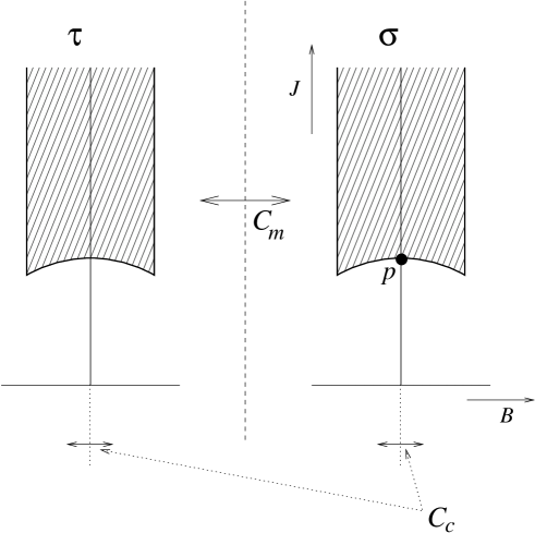
Figure 3: Moduli Space of a Torus.

In particular if we consider the example of section 3.3.4 then we have a Narain factor of the form

$$\operatorname{O{}}(\Gamma_{2,2})\backslash\operatorname{O{}}(2,2)/(\operatorname{O{}}(2)\times\operatorname{O{}}(2))\cong(C_{m}\times C_{c})\backslash\left(\frac{\mathsf{H}_{\sigma}}{\operatorname{SL}(2,{\mathbb{Z}})}\times\frac{\mathsf{H}_{\tau}}{\operatorname{SL}(2,{\mathbb{Z}})}\right).$$ (64)

Here we have used the standard decomposition of the Grassmannian into a form which makes it more recognizable for our purposes. We have two copies of the upper half-plane $\mathsf{H}\cong\operatorname{SL}(2,{\mathbb{R}})/\operatorname{U{}}(1)$ which we parameterize by complex numbers $\sigma$ and $\tau$ respectively. The groups $C_{m}$ and $C_{c}$ are both isomorphic to ${\mathbb{Z}}_{2}$ and are generated by

$$\begin{split}g_{m}:(\tau,\sigma)&\mapsto(\sigma,\tau)\\ g_{c}:(\tau,\sigma)&\mapsto(-\bar{\tau},-\bar{\sigma}),\end{split}$$ (65)

respectively. We refer to [98], for example, for details of this isomorphism. We depict this moduli space in figure 3.

The interpretation of this moduli space in terms of $E_{H}$ is straight-forward. We let $\tau$ denote the complex structure in the standard way and we let $\sigma$ denote the single component of $B+iJ$.

Thus the $\operatorname{SL}(2,{\mathbb{Z}})$ action on $\tau$ is the standard modular invariance of a 2-torus. The $\operatorname{SL}(2,{\mathbb{Z}})$ acting on $\sigma$ is composed of the familiar $B\to B+1$ symmetry as well as a $J\to 1/J$ T-duality. Note that $C_{m}$ is “mirror symmetry” for a 2-torus as was first seen in [99]. $C_{c}$ can be thought of as a complex conjugation symmetry of the theory.

This is all very well but we have noticed in the previous section that this picture of the moduli space is subject to quantum corrections. That is, this Narain picture of the moduli space of $E_{H}$ is not exact. We will now argue that the effect of these quantum corrections is to completely ruin the description of the moduli space as a quotient and so any notion of T-duality for $E_{H}$ is lost.

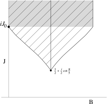
Figure 4: Moduli Space of the Quintic.

To argue this let us discuss what can go wrong with T-duality arguments in another example. We will consider the classical quintic hypersurface in ${\mathbb{P}}^{4}$ as was analyzed in [72]. The Calabi–Yau manifold has $h^{1,1}=1$. When we flatten out the single complex coordinate describing $B+iJ$ we obtain the moduli space depicted in figure 4. Now although this moduli space looks similar to the fundamental region of $\mathsf{H}/\operatorname{SL}(2,{\mathbb{Z}})$ there is a big difference. There is no action of any discrete group on $\mathsf{H}$ for which the region in figure 4 is a fundamental region. One may see this as follows. Note that there is an angle of $2\pi/5$ formed at the lowest point in this region. One should therefore need 5 fundamental regions touching at this point. Indeed one may find such regions and they are pictured in figure 5.2 of [72]. One can also see that the $B\to B+1$ symmetry should allow us to translate these fundamental regions one unit to the left or right to form new fundamental regions. The problem is that doing this translation gives a region which overlaps in an open set with one the regions we built earlier by rotating by $2\pi/5$. Thus these supposed fundamental regions do not tessellate in $\mathsf{H}$ and therefore cannot be derived in terms of a group action on $\mathsf{H}$.

Indeed we argued in section 2 that $N=2$ theories in four dimensions do not generically have locally symmetric moduli space. It was in the context of symmetric spaces that we saw the natural appearance of T-duality. It should not therefore be a surprise that we do not find the true analogue of a modular group for the quintic threefold.

We should therefore expect that the quintic threefold represents the generic case of a Calabi–Yau moduli space. In particular once we turn on the heterotic string coupling, i.e., give finite size to the section $W$ of the example in section 3.3.4 the Narain description of the moduli space is lost. This is argued in [7].

So if the heterotic string on a torus does not respect T-duality how should we really describe the moduli space? The principle should be the same as that for the quintic threefold. One should begin with a weakly coupled heterotic string on a large circle or torus. Here one unambiguously sees the geometry of the compactification. Now move about the moduli space of compactifications. In this we can label every point in the moduli space by a set of moduli (such as radii) for the torus. One problem we have to be careful about is that we may follow loops in the moduli space which allow us to identify more than one torus with a given point in the moduli space of theories. We must avoid this by putting cuts in the moduli space. If we do not put in such cuts then generically one would expect to be able to identify every possible torus with each point in the moduli space! (Note that since the classical $\operatorname{SL}(d,{\mathbb{Z}})$ symmetry of a $d$-torus is lost one must describe the torus directly in terms of data which chooses a fundamental region of the classical moduli space of flat metrics.)

Once we have completed this labelling process (the details of which depend on a choice of cuts) we have defined every possible torus to be considered. Tori excluded by the process, such a circle of radius less that $\sqrt{\alpha^{\prime}}$, do not exist and should not be considered. It is only the accidental T-duality of the weakly-coupled string that led us to believe that we could make real sense of small tori.

• This example consisted of a moduli space ${\Scr M}_{V}$ which became locally a symmetric space on its boundary at infinite distance corresponding to some classical limit. It is interesting to note that there are other known examples where a subspace of ${\Scr M}_{V}$ can be locally symmetric. For example consider the so-called Z-orbifold $T^{6}/{\mathbb{Z}}_{3}$ with 27 fixed points. The rational curves in this space (after blowing up) conspire to only give certain quantum corrections to ${\Scr M}_{V}$. The effect of this is to make the prepotential ${\Scr F}$ exactly cubic if none of the 27 blow-up modes are switched on [100]. The result is that we get a slice of the moduli space (at finite distance) of the form

  $${\Scr M}_{V,\mathrm{orb}}\cong\operatorname{U{}}(3,3;{\mathbb{Z}})\backslash\operatorname{U{}}(3,3)/(\operatorname{U{}}(3)\times\operatorname{U{}}(3)).$$ (66)

  Moving away from this subspace there are instanton corrections and the symmetric space structure is lost.

Note that in general we lose the classical $\operatorname{SL}(2,{\mathbb{Z}})$ symmetry of the complex structure of the torus in addition to any T-duality. How can this be?

The moduli space of a 2-torus of volume one is determined by considering the ways of making a a lattice of area one, dividing out by rotations, and then dividing out by the modular group $\operatorname{SL}(2,{\mathbb{Z}})$. This gives us the familiar form $\operatorname{SL}(2,{\mathbb{Z}})\backslash\operatorname{SL}(2,{\mathbb{R}})/\operatorname{SO}(2)$. If we declare that quantum effects break this structure then quantum effects must be having a drastic effect on this construction of the torus. As well as breaking the $\operatorname{SL}(2,{\mathbb{Z}})$ invariance, we are also modifying the $\operatorname{SL}(2,{\mathbb{R}})/\operatorname{SO}(2)$ part. It is as if we are breaking the picture of the 2-torus as a Riemannian manifold. Hopefully once stringy geometry is better-understood it will be more clear what is happening here.

It is worth mentioning that there are two distinct types of U-dualities discussed in the literature. One is an “internal duality” statement where one says that a string theory of type $\Scr{S}_{1}$ (e.g., type IIA, $E_{8}\times E_{8}$ heterotic etc.) compactified on $X_{1}$ with coupling $\lambda_{1}$ is dual to a string theory of the same type $\Scr{S}_{1}$ compactified on $X_{2}$ with coupling $\lambda_{2}$. Alternatively one has an “external duality” where one says that a string theory of type $\Scr{S}_{1}$ compactified on $X_{1}$ with coupling $\lambda_{1}$ is dual to a string theory of a different type $\Scr{S}_{2}$ compactified on $X_{2}$ with coupling $\lambda_{2}$.

Our discussion of the breaking of T-dualities (and by implication U-dualities) was in the context of internal dualities. In particular we were fixing our string as an $E_{8}\times E_{8}$ heterotic string. What happens when the external duality relating an $E_{8}\times E_{8}$ heterotic string on a given torus and a given choice of Wilson lines to a $\operatorname{Spin}(32)/{\mathbb{Z}}_{2}$ heterotic string on another torus and set of Wilson lines?

Our discussion of mapping out the moduli space should apply again. Map out the moduli space of tori and Wilson lines as above using the $E_{8}\times E_{8}$ heterotic string. Now do the same thing with the $\operatorname{Spin}(32)/{\mathbb{Z}}_{2}$ heterotic string. Note that the starting point for the large torus will not be the same limit point in moduli space as the former case. This means that every point in the moduli space will now have two labels — one for each heterotic string. One should not obtain small radii for either heterotic string interpretation.

Thus strictly external U-dualities need not be broken by quantum effects. The precise mapping between $(X_{1},\lambda_{1})$ and $(X_{2},\lambda_{2})$ can be expected to be modified however.

4 The Moduli Space of Hypermultiplets

Now we come to the considerably more tricky subject of trying to map out the moduli space of hypermultiplets for our $N=2$ theories in four dimensions. In the case of the vector multiplet moduli space, the type IIB string compactified on $Y$ gave an exact model. For the hypermultiplets there is no exact model. This makes the subject much more difficult and potentially much more interesting!

4.1 Related Dimensions

The purpose of these lectures is to discuss some special properties of $N=2$ theories in four dimensions. It turns out to be very useful to be aware of some other closely-related theories in both higher and lower dimensions than four to help gain insight into the hypermultiplet moduli space.

4.1.1 $N=(1,0)$ in six dimensions

Imagine compactifying the heterotic string on a K3 surface $S_{H}$. This would yield a theory with $N=(1,0)$ supersymmetry in six dimensions. We refer the reader to [101] for a good discussion of many aspects of such theories. This has an $R$-symmetry of $\operatorname{Sp}(1)$. We discussed the supermultiplets of such theories in section 2.3. Such a theory may then be compactified on a 2-torus to yield our familiar $N=2$ theory in four dimensions. Upon dimensional reduction, the $N=(1,0)$ supermultiplets in six dimensions become $N=2$ supermultiplets in four dimensions as follows:

• A six-dimensional hypermultiplet becomes a hypermultiplet in four dimensions.

• A six-dimensional vector multiplet becomes a vector multiplet in four dimensions.

• A six-dimensional tensor multiplet becomes a vector multiplet in four dimensions.

In particular the hypermultiplet moduli space of a heterotic string compactified on a K3 surface $S_{H}$ is exactly the same as the hypermultiplet moduli space of a heterotic string compactified on $S_{H}\times E_{H}$. This is consistent with our earlier comment that all the hypermultiplet information comes from the K3 surface $S_{H}$.

It is therefore quite common to analyze the hypermultiplet moduli space in terms of six-dimensional physics rather than four-dimensional physics. Having said that, our duality statements might now sound a bit peculiar. We want to say something to the effect that we can model the hypermultiplet moduli space of a heterotic string on a K3 surface in terms of a type IIA string on a Calabi–Yau threefold $X$ but the former is six-dimensional while the latter is four-dimensional.

It is important to note that we cannot necessarily completely ignore the 2-torus $E_{H}$ in the product $S_{H}\times E_{H}$. In effect we can think of arriving at our six-dimensional theory by beginning in four dimensions and decompactifying $E_{H}$. To do this we certainly need the full moduli space of $E_{H}$ and from proposition 10 this in turn implies that the Calabi–Yau threefold $X$ is an elliptic fibration with a section. Assuming this is the case, we may model the six-dimensional physics of the heterotic string on $S_{H}$ in terms of the type IIA string on $X$ by implicitly decompactifying $E_{H}$.

Figure 5: Classification of elliptic fibres.

This mechanism of using type IIA strings on $X$ to model six-dimension physics is known as “F-theory”. The reader should be warned that there are at least two other ways of defining F-theory common in the literature. One is to treat F-theory as twelve dimensional (although whether it lives in ${\mathbb{R}}^{2,10}$ or ${\mathbb{R}}^{1,11}$ is unclear). Another way is to view it as a type IIB string compactification with a varying dilaton. We refer to [102, 103] for more details. The type IIA definition of F-theory is well-suited for our purposes of linking the subject to four dimensions.

Let us denote the elliptic fibration as $p:X\to\Theta$, where $\Theta$ is a complex surface. We also know we have a K3-fibration $\pi:X\to W$, where $W\cong{\mathbb{P}}^{1}$, and a fibration $\Theta\to W$ with generic fibre given by ${\mathbb{P}}^{1}$. That is, $\Theta$ is a “ruled surface”. If $\Theta$ is a smooth ${\mathbb{P}}^{1}$-bundle over $W$, it is the “Hirzebruch surface” ${\bf F}_{n}$. Here the section $W\hookrightarrow\Theta$ has self-intersection $-n$ within $\Theta$. Blowing up ${\bf F}_{n}$ at a few points replaces some of the smooth ${\mathbb{P}}^{1}$-fibres by chains of ${\mathbb{P}}^{1}$’s.

It is common to then draw $X$ (representing a complex dimension as a real dimension) in the following form. We may use the plane of the paper to represent $\Theta$ by letting the horizontal direction represent the section and the vertical direction represent the ${\mathbb{P}}^{1}$-fibre. That is, the “ruling” of the ruled surface $\Theta$ is given by vertical lines. Now over a (complex) codimension one subspace of $\Theta$ the elliptic fibration $p:X\to\Theta$ will degenerate. We may draw this “discriminant” locus as a set of curves and lines in the plane of the paper.

Kodaira has classified the possibilities for how an elliptic fibre may degenerate in the case of one parameter family [104]. We show the possibilities in figure 5. With the exception of $\mathrm{I}_{0}$ which is the smooth elliptic case, and $\mathrm{II}$ which is an elliptic curve with a cusp, each line in the figure represents a rational curve. This curve may appear with a multiplicity given by the small numbers in the figure. This classification can be used to label the generic points on the irreducible components of the discriminant locus.

Figure 6: A typical elliptic fibration.

The result is that one obtains a picture somewhat typically like figure 6 for $X$ in the form of an elliptic fibration. In this figure the dotted lines represent lines (${\mathbb{P}}^{1}$’s) within $\Theta$. $C_{0}$ is a section and $f$ is a generic ${\mathbb{P}}^{1}$ fibre. Note that this notation is consistent with the $f$ which appeared in section 3.3.4. At one point over $W$ we have put a fibre as a chain of three ${\mathbb{P}}^{1}$’s. The solid lines represent the discriminant locus. Each irreducible component is labelled by its Kodaira type. When these components collide, the elliptic fibration will degenerate further and the resulting fibre need not lie in Kodaira’s classification.

Since we wish to study the moduli space of hypermultiplets we are particularly interested in the deformations of complex structure of $X$. When we draw $X$ as an elliptic fibration, the complex structure is encoded in the discriminant locus. Thus, deformations of $X$ are given simply by the deformations of the discriminant locus.

It will also be worthwhile to note how the Kähler form data appears in the elliptic fibration. Deforming the Kähler form may either affect areas in the fibre direction (i.e., the area of the generic fibre as well as areas within the chains of special Kodaira fibres) or affect areas within $\Theta$. As we decompactify $E_{H}$ to go from 4 dimensions to 6 dimensions one can show that the areas in the fibre direction become meaningless [105, 1]. Our discussion of the types of supermultiplets in four and six dimensions given at the start of this section leads one to conclude:

• Using the Kähler form to vary areas in the fibre direction corresponds to moduli in a six-dimensional vector supermultiplet.

• Using the Kähler form to vary areas in $\Theta$ corresponds to moduli in a six-dimensional tensor supermultiplet.

4.1.2 $N=4$ in three dimensions

Imagine taking our $N=2$ theory in four dimension and compactifying further on a circle. This leads to a theory in three dimensions with $N=4$ supersymmetry. This has an $R$-symmetry of $\operatorname{SO}(4)\cong\operatorname{Sp}(1)\times\operatorname{Sp}(1)$ (up to irrelevant discrete factors) which implies that the moduli space should factorize into a product of two quaternionic Kähler spaces. These three dimensional theories have two different types of “hypermultiplets” whose moduli spaces cannot mix. In the literature one often refers to one of these types of hypermultiplets as “vector multiplets” to reflect their four-dimensional origin. However, one should be aware that, within the context of the three-dimensional physics, such a distinction is arbitrary.

Note that the hypermultiplet moduli space ${\Scr M}_{H}$ from four dimensions comes through unscathed into the three dimensional picture whereas our vector multiplet moduli space becomes “quaternionified” in the compactification. It is remarkable how resilient ${\Scr M}_{H}$ is! It is unchanged as we compactify on circles a theory in six dimensions with $N=(1,0)$ supersymmetry down to three dimensions. Compare this with the capricious vector multiplet moduli space which is non-existent in 6 dimensions, real in 5 dimensions, complex in 4 dimensions and quaternionic in 3 dimensions!

Because the vector multiplet moduli space becomes a hypermultiplet moduli space upon compactification to three dimensions, this picture provides a potentially useful way of using our knowledge of special Kähler manifolds to uncover some of the mysteries of quaternionic Kähler manifolds.

Suppose we wish to study ${\Scr M}_{H}(X)$ for a type IIA string compactified on the Calabi–Yau threefold $X$. Consider instead the moduli space ${\Scr M}_{V}(Y)$ of the type IIA string compactified on $Y$, the mirror of $X$. Compactifying further on $S^{1}_{R}$, a circle of radius $R$, the special complex Kähler space ${\Scr M}_{V}(Y)$ becomes a quaternionic Kähler space which we will denote ${\Scr M}_{V}(Y)_{\mathbb{H}}$. Since the type IIA string on a circle of radius $R$ is supposedly T-dual to the type IIB string on a circle of radius $1/R$, the type IIA string on $Y\times S^{1}_{R}$ should be dual to the type IIB string on $Y\times S^{1}_{1/R}$. Using mirror symmetry this is then dual to the type IIA string on $X\times S^{1}_{1/R}$. The space ${\Scr M}_{V}(Y)_{\mathbb{H}}$ must now represent the factor of the moduli space containing deformations of complex structures of $X$. That is, it descended from ${\Scr M}_{H}(X)$ upon compactification on the circle. Having said that, ${\Scr M}_{H}(X)$ is unchanged by this circle compactification and so

$${\Scr M}_{H}(X)\cong{\Scr M}_{V}(Y)_{\mathbb{H}}.$$ (67)

• We already questioned the validity of T-duality for the heterotic string in section 3.3.6. It is natural to question whether T-duality is valid for the type II strings when we have only modestly extended supersymmetry. The crude statement that the type IIA string compactified on $Y\times S^{1}_{R}$ is dual to the type IIB string compactified on $Y\times S^{1}_{1/R}$ is almost certainly incorrect. It is true however that one should expect this to be exact when the strings are very weakly coupled. Most analyses of strings using this statement of T-duality such as [106] do use only weakly-coupled strings. We will not try to elucidate the exact meaning of T-duality in type II strings in these lectures.

Determining ${\Scr M}_{V}(Y)_{\mathbb{H}}$ from the complex space ${\Scr M}_{V}(Y)$ is not easy. An interesting attempt at this problem was made some time ago by Cecotti et al. in [107]. This paper assumed that the moduli space ${\Scr M}_{V}$ was determined by a prepotential that was exactly cubic. Particular attention was paid to the cases where ${\Scr M}_{V}$ is a symmetric space. If one then ignored quantum corrections upon compactification on a circle, this symmetric space was mapped via the so-called “$c$-map” to another symmetric space. For example one might have something like

$$c:\frac{\operatorname{SU}(3,3)}{\mathrm{S}(\operatorname{U{}}(3)\times\operatorname{U{}}(3))}\to\frac{E_{6(+2)}}{\operatorname{SU}(2)\times\operatorname{SU}(6)}.$$ (68)

A notable case of the $c$-map is

$$c:\frac{\operatorname{SL}(2,{\mathbb{R}})}{\operatorname{U{}}(1)}\times\frac{\operatorname{SO}_{0}(2,n-2)}{\operatorname{SO}(2)\times\operatorname{SO}(n-2)}\to\frac{\operatorname{SO}_{0}(4,n)}{\operatorname{SO}(4)\times\operatorname{SO}(n)}.$$ (69)

We will revisit this briefly in section 4.4.3.

Of course, unless we pick a very special model to examine, there will be quantum corrections and the analysis of [107] will not be directly applicable. However, this method may provide a good starting point for the analysis of the quaternionic Kähler moduli spaces as it does give the asymptotic behaviour where quantum effects can be neglected.

An exact version of the $c$-map was elucidated by Seiberg and Witten [61] in the case of rigid special Kähler geometry. As discussed in section 3.3.5, ${\Scr M}_{V}(Y)$ is described in this limit by the deformation of a complex curve $C_{\mathrm{SW}}$. Seiberg and Witten’s remarkably simple result is then

Proposition 13

In the case that ${\Scr M}_{Y}(V)$ is a rigid special Kähler space, ${\Scr M}_{V}(Y)_{\mathbb{H}}$ is simply the hyperkähler space given by an abelian (i.e., complex algebraic torus) fibration over ${\Scr M}_{V}(Y)$ where the fibre is given by the Jacobian $H^{1}(C_{\mathrm{SW}},\operatorname{U{}}(1))$. In addition the volume of the fibre is determined by $R$, the radius of the circle on which one compactifies.

4.2 Extremal Transitions

Since direct analysis of the hypermultiplet moduli space is so formidable the most prudent course of action is to try to squeeze as much information out of our knowledge of the vector multiplet moduli space as we possible can.

This is facilitated by the occurrence of phase transitions or “extremal transitions”. We go to a funny point in moduli space where vector moduli disappear and new hypermultiplet moduli appear. We may then pretend that we actually did this process in reverse and claim that we know something about what happens when we move around in the moduli space of hypermultiplets!

4.2.1 Conifolds

Let us consider the simplest type of extremal transition first — the “conifold” of [109]. We may understand this both from the point of view of geometry and from the point of view of field theory as explained in [110, 111].

We begin with the geometrical picture. Consider the type IIB string compactified on the Calabi–Yau manifold $Y$. We move about the moduli space of vector multiplets by deforming the complex structure of $Y$. Let us consider a one-dimensional family of such $Y$’s and denote an element of this family by $Y_{t}$ where $t$ parameterizes the family. At a special point in this part of the moduli space, say $t=0$, $Y$ may become singular. The simplest thing that can happen as $t\to 0$ is that an $S^{3}$ can contract to a point. Locally such a singularity would look like the hypersurface

$$w^{2}+x^{2}+y^{2}+z^{2}=0,$$ (70)

in ${\mathbb{C}}^{4}$. This is called a “conifold singularity”.

Locally such a conifold point can be resolved by replacing the point by a ${\mathbb{P}}^{1}$ (see, for example, [109] for a nice explanation of this). Since the Kähler form controls the areas of ${\mathbb{P}}^{1}$’s such a resolution might be pictured as a deformation of Kähler form. In other words we have turned a degree of freedom from a deformation of complex structure into a deformation of Kähler form.

Globally this picture does not work quite this simply. We need to consider the case of $P$ disjoint $S^{3}$’s, each shrinking to a point at $t=0$. If $Y_{t}$ represents the smooth $Y$ for a generic value of $t$ then a simple application of the Mayer-Vietoris sequence gives a relationship between the homology of $Y_{t}$ and the homology of $Y_{0}$. See [112] for a full description of this process.

Now resolve the resulting $P$ conifold points by adding ${\mathbb{P}}^{1}$’s and call the resulting smooth manifold $Y^{\prime}$. Another application of the Mayer-Vietoris sequence gives a relationship between the homology of $Y_{0}$ and the homology of $Y^{\prime}$. Combining these results we obtain

$$\begin{split}0\to H_{4}(Y_{t})\to H_{4}(Y^{\prime})\mathrel{\mathop{\to}^{f_{1}}}&\,{\mathbb{Z}}^{P}\to H_{3}(Y_{t})\to H_{3}(Y_{0})\to 0\\ 0\to H_{3}(Y^{\prime})\to H_{3}(Y_{0})\to&\,{\mathbb{Z}}^{P}\mathrel{\mathop{\to}^{f_{2}}}H_{2}(Y^{\prime})\to H_{2}(Y_{t})\to 0.\end{split}$$ (71)

Let us denote by $Q$ the rank of the map labelled $f_{1}$. By Poincaré duality the rank of $f_{2}$ must also then be $Q$. Note that $Q$ represents the dimension of the kernel of the map ${\mathbb{Z}}^{P}\to H_{3}(Y_{t})$, i.e., the number of homology relations between the $P$ 3-spheres in the smooth $Y$. The above exact sequences give

$$\begin{split}b_{2}(Y^{\prime})&=b_{2}(Y_{t})+Q\\ b_{3}(Y^{\prime})&=b_{3}(Y_{t})-2(P-Q).\end{split}$$ (72)

That is, as we go through the conifold transition, we lose $P-Q$ vector multiplets and gain $Q$ hypermultiplets. Note that $P>1$ is required for this transition to make sense and so a single conifold point is not sufficient.

From the point of view of field theory this process is a supersymmetric variant of the Higgs mechanism. As we wander about the moduli space of vector multiplets it is possible that some hypermultiplets suddenly become massless. Indeed, Strominger [110] noted that the singularities in the moduli space metric associated to a conifold are exactly the same as seen by Seiberg and Witten when a hypermultiplet becomes massless.

Suppose $P$ hypermultiplets become massless and that these hypermultiplets are charged under $P-Q$ of the $\operatorname{U{}}(1)$ gauge symmetries in our original theory. We may try to give these new hypermultiplets vacuum expectation values which would then spontaneously break this $\operatorname{U{}}(1)^{P-Q}$ gauge symmetry. Our $N=2$ gauge theory in four dimensions has the standard gauge theory couplings and so these broken gauge symmetries must “eat up” some Goldstone bosons in order to become massive. What’s more they must do this in a way consistent with $N=2$ supersymmetry. The only way this can happen is for us to lose $P-Q$ of our $P$ new massless hypermultiplets leaving us with $Q$ new hypermultiplets. This is the field theory picture for losing $P-Q$ vector multiplets and gaining $Q$ hypermultiplets.

Since we obtain $Y^{\prime}$ via the Higgs mechanism, this is often referred to as the “Higgs phase”. Since $Y_{t}$ has more $\operatorname{U{}}(1)$’s (massless photons) it is referred to as the “Coulomb phase”. That is, the Higgs phase is the one with more hypermultiplets and the Coulomb phase is the one with more vector multiplets.

The conifold transition is just the simplest example of all kinds of extremal transitions which may occur.

4.2.2 Enhanced gauge symmetry

The Higgs phase transition of the preceding section was a little boring because there was no nonabelian gauge symmetry at the phase transition point. We know how to get enhanced gauge symmetry (at least in some limit) from section 3.3.3. We need to consider the type IIA string compactified on $X$, where $X$ has a curve of ADE singularities.

This is easy to arrange using the elliptic fibration language of section 4.1.1. We can describe the situation using the “Weierstrass form” of the elliptic fibration which is standard when discussing F-theory. Let $s$ and $t$ be affine complex coordinates on some patch of the base $\Theta$. We may then write the elliptic fibration as

$$y^{2}=x^{3}+a(s,t)x+b(s,t).$$ (73)

The discriminant is then given by $\Delta=4a^{3}+27b^{2}$. The geometry of such fibrations was discussed in detail in [1] and so we will be brief here.

$$\begin{array}[]{|c|c|c|c|c|}\hline\cr L&K&N&\mbox{Fibre}&\mbox{Sing.}\\ \hline\cr\geq 0&\geq 0&0&{\rm I}_{0}&\\ 0&0&>0&{\rm I}_{N}&A_{N-1}\\ \geq 1&1&2&{\rm II}&\\ 1&\geq 2&3&{\rm III}&A_{1}\\ \geq 2&2&4&{\rm IV}&A_{2}\\ \geq 2&\geq 3&6&{\rm I\vphantom{\rm II}}^{*}_{0}&D_{4}\\ 2&3&\geq 7&{\rm I\vphantom{\rm II}}^{*}_{N-6}&D_{N-2}\\ \geq 3&4&8&{\rm IV}^{*}&E_{6}\\ 3&\geq 5&9&{\rm III}^{*}&E_{7}\\ \geq 4&5&10&{\rm II}^{*}&E_{8}\\ \hline\cr\end{array}$$

Table 3: Weierstrass classification of fibres.

Let us assume $a$ and $b$ are independent of $t$ for the time being. We wish to put a line of interesting fibres along $s=0$. Table 3 lists the resulting fibres where $a\cong s^{L}$, $b\cong s^{K}$ and $\Delta\cong s^{N}$ near $s=0$. The final column denotes the resulting singularity if all the components of the fibre not intersecting the section are shrunk down to zero area. Note that the fibres $\mathrm{I}_{0}$, $\mathrm{I}_{1}$ and II only have one component and thus cannot produce a singularity.

This results in an explicit description of an extremal transition involving nonabelian gauge symmetry. Begin with a type IIA string on a smooth Calabi–Yau threefold $X$ where all the components of all the fibres have nonzero area. Now shrink down all the components of the fibres which do not hit the section. This will result in curves of ADE singularities producing some gauge group ${\Scr G}$. We may then be free to deform the discriminant by a deformation of complex structure to smooth the threefold.

Let us recast this transition in terms of the language of a heterotic string compactified on $S_{H}\times E_{H}$. The process begins by a deformation of the Kähler form of $X$ which is thus a deformation of the bundle over $E_{H}$ (or $E_{H}$ itself). That is, we vary Wilson lines over $E_{H}$. We then obtain the gauge group ${\Scr G}$ by switching these lines “off”. The deformation of complex structure of $X$ then corresponds to deforming the bundle over the K3 surface $S_{H}$ to reabsorb the enhanced gauge symmetry ${\Scr G}$ into a bundle.

This extremal transition therefore appears as reducing the structure group of the bundle $V_{E}\to E_{H}$ and increasing the structure group of $V_{S}\to S_{H}$.

We begin in the “Coulomb” branch where ${\Scr G}$ is broken to its Cartan subgroup $\operatorname{U{}}(1)^{\operatorname{rank}({\Scr G})}$. We end up in the “Higgs” branch where ${\Scr G}$ may be completely broken. This process therefore decreases the number of vector multiplets as one would expect.

An interesting point to bear in mind is that the gauge group ${\Scr G}$ can be broken by quantum effects, i.e., effects due to $\lambda$-corrections in the heterotic string and $\alpha^{\prime}$-corrections (specifically worldsheet instantons wrapped around the base $W$) in the type IIA string. Even though ${\Scr G}$ is broken however it does not mean that the phase transition cannot happen. Quantum effects cannot obstruct motion in the moduli space and these extremal transitions most certainly exist in terms of Calabi–Yau threefolds.

What tends to happen, as explained in [88], is that the phase transition point does not happen at a point of enhanced gauge symmetry (which need not exist) but rather at a point where some solitons become massless. Only if quantum effects are ignored would these solitons actually produce the enhanced gauge symmetry.

In a particularly interesting class of examples the extremal transition can become more complicated. One may have more than one Higgs phase joining on to the Coulomb branch. This is actually understood both in terms of field theory and in terms of the geometry of Calabi–Yau threefolds. An example of a field theory with two Higgs branches was discussed in [88]. The geometry was explained in [58] based on an earlier observation by Gross [113].

As mentioned above, when we go to the six-dimensional picture of this field theory, the degrees of freedom associated to the areas of the elliptic fibration $p:X\to\Theta$ become frozen. That is, the vector supermultiplets associated to the above gauge groups lose their moduli. Because of this we lose the Coulomb branch of the theory. In other words there are special points in ${\Scr M}_{H}$ where we may acquire enhanced gauge symmetry but there is never any phase transition associated with such events.

4.2.3 Massless Tensors

Having said that we lose the standard Higgs-Coulomb phase transitions associated to enhanced gauge symmetry when we look at six dimensional $N=(1,0)$ theories, one may ask if we have any transitions at all. There are indeed still interesting phase transitions in six dimensions as was explained in [101].

Going to the six dimensional decompactification limit of the four dimensional theories may freeze out the Kähler form degrees of freedom associated to the fibres of $p:X\to\Theta$, but there are still Kähler degrees of freedom remaining within $\Theta$ itself.

Since these degrees of freedom are present as moduli in six dimensions and descend to vector multiplet moduli in four dimensions, they must be associated to scalars living in the six-dimensional tensor multiplets [105].

Note that the scalar fields in tensor multiplets have only one real degree of freedom. There is no modulus associated to varying the $B$-field on $\Theta$. Effectively the periodicity of $B$ tends to zero as we decompactify the four dimensional theory to six dimensions. The geometry of the tensor moduli space is given by the real special Kähler geometry of section 3.2.1.

The six-dimensional phase transitions are then between a phase spanned by hypermultiplets, which we still call the Higgs phase, and a phase spanned by tensor multiplets, which is called the Coulomb phase for consistency with the four-dimensional picture.

In terms of F-theory on a Calabi–Yau threefold $X$ this phase transition is really nothing more than the conifold transition we discussed in section 4.2.1. We will give an example here to explicitly give the geometry of the elliptic fibration. For more details on the geometry we refer to [1].

Consider an elliptic fibration whose local Weierstrass form is

$$y^{2}=x^{3}+s^{4}x+s^{5}t.$$ (74)

This has a type $\mathrm{II}^{*}$ fibre running along $s=0$ and so one would associate this to an $E_{8}$ gauge group. At $t=0$ something special happens. The elliptic fibration degenerates so badly that the only fibre that would smooth the space out would actually be complex dimension two rather than some algebraic curve. To avoid this one may blow up the point $s=t=0$ in the base to introduce a new rational curve into $\Theta$. One is certainly not always free to do this! Blowing up any old point in $\Theta$ would usually result in breaking the Calabi–Yau condition. It is only because (74) is so singular that one can do this.

The form (74) is therefore precisely at the phase transition point. We may go off into the Higgs phase by deforming the equation, and thus the complex structure of $X$. We may go off into the Coulomb phase by blowing up the base $\Theta$ at $s=t=0$.

4.3 The classical limit

The preceding section on extremal transitions gives us invaluable information about specific points in ${\Scr M}_{H}$ — those which allow phase transitions into new dimensions in ${\Scr M}_{V}$. We now explore the other part of ${\Scr M}_{H}$ which is accessible. We will look at the boundary where all quantum effects may be ignored.

We have asserted that the heterotic string compactified on $(V_{S}\to S_{H})\times(V_{E}\to E_{H})$ is dual to the type IIA string compactified on a Calabi–Yau threefold $X$. If we could go to a limit in the moduli space where the $\alpha^{\prime}$-corrections to the heterotic string and the $\lambda$-corrections to the type IIA string were simultaneously switched off then we should be able to map the two respective moduli spaces of hypermultiplets exactly onto each other.

In order to completely ignore $E_{H}$ and its bundle we will assert that we are in the F-theory situation where $X$ is a K3 fibration and an elliptic fibration with a section. We will also demand that $S_{H}$ is itself an elliptic surface with a section. This latter demand kills many moduli and one might ask whether one really needed to impose such a drastic constraint. As we will see, it appears to be necessary to get a simple description of the classical moduli spaces.

In proposition 8 of section 3.3.2 we showed that the dilaton of the heterotic string is mapped to the area of the ${\mathbb{P}}^{1}$ base of $X$ as a K3-fibration. While we tried to be quite rigorous in showing proposition 8, there is a quicker (but dirtier) way showing the same thing. Suppose that $X$ were not a K3-fibration over ${\mathbb{P}}^{1}$ but simply a product of a K3 surface times an elliptic curve. This would yield an $N=4$ theory in four dimensions. It is also dual to a heterotic string on $T^{6}$. One may then use a simple dimensional reduction argument [114, 115, 116] to show that the coupling of the heterotic string is given by the area of the elliptic curve on which the type IIA string was compactified. The same argument shows that the coupling of the type IIA string is given by the area of one of the $T^{2}$’s in the heterotic 6-torus.

If we assume that $T^{2}\times Q$ (for any space $Q$) is equivalent to a $Q$-fibration over ${\mathbb{P}}^{1}$ as far as areas are concerned then this simple dimensional reduction argument reproduces proposition 8. It also implies that the coupling of the type IIA string is determined by the area of the section of the K3 surface $S_{H}$, as an elliptic fibration, on which the heterotic string is compactified.

We will assume this statement is true even though this argument considerably lacks rigour. See [117] for a more thorough treatment of this question.

In order to make the type IIA string very weakly coupled we are therefore required to make the section of $S_{H}$ very large on the heterotic side. This will eliminate $\lambda$-corrections on the type IIA side. Now in order to remove the $\alpha^{\prime}$-corrections on the heterotic side we are required to make the K3 surface $S_{H}$ very large. Since we have made the section of $S_{H}$ large we have already fulfilled this requirement partially.

If we assume that $S_{H}$ is a completely generic elliptic K3 surface with a section, then the only other area we need care about is that of the generic elliptic fibre. If both the section and the fibre have large area then every minimal 2-cycle in $S_{H}$ will be large, unless we have chosen to be close to a special point in the moduli space of Ricci-flat metrics where a 2-cycle shrinks down to zero size.

How exactly we take the area of the generic fibre of $S_{H}$ to be infinite was first explained in [23] following an observation in [103]. It was then explored more fully in [118, 119]. We refer the reader to [118, 119] for details of the following argument. We will approach this problem as an algebraic geometer would. For a discussion of the link of this approach with a more metric-minded picture see [120].

Figure 7: The $E_{8}\times E_{8}$ stable degeneration.

The basic idea is that taking the areas of the fibres of $S_{H}$ to be large corresponds to a deformation of complex structure of $X$. There is therefore some limiting complex structure of $X$ which represents $S_{H}$ at infinite size. We may construct this by considering a one-dimensional family of $X$’s. Let $w:{\Scr X}\to D$ be a fibration of some 4-dimensional complex manifold ${\Scr X}$ over some complex disc $D$. Let $u$ be a complex parameter for $D$. If $u\neq 0$ then the the fibre $w^{-1}(u)$ will be a smooth Calabi–Yau threefold in the class $X$. When $u=0$, our fibre $X_{0}$ will be singular. It is $X_{0}$ which will correspond to $S_{H}$ with a generic elliptic fibre of infinite area.

4.3.1 The $E_{8}\times E_{8}$ heterotic string

In order to proceed further we need to specify whether we are talking about the $E_{8}\times E_{8}$ heterotic string or the $\operatorname{Spin}(32)/{\mathbb{Z}}_{2}$ heterotic string. We will deal with the $E_{8}\times E_{8}$ case first.

A picture of what happens as $X$ turns into $X_{0}$ is depicted in figure 7 for the case of the $E_{8}\times E_{8}$ heterotic string. What happens is that the Calabi–Yau threefold $X$ “breaks in two” to give a reducible space $X_{1}\cup X_{2}$ intersecting along a complex surface $S_{*}$. This surface is an elliptic fibration over a ${\mathbb{P}}^{1}$ which we denote $C_{*}$ in figure 7. The surface $S_{*}$ is in fact a K3 surface and is isomorphic to $S_{H}$!

The way one shows this is via an adiabatic argument where one thinks of $S_{H}$ as a slowly-varying elliptic fibration. One then focuses attention on one elliptic fibre and pretends that the heterotic string compactified on this single fibre is dual to F-theory on a K3 surface. Such an adiabatic argument might be considered a little dangerous when trying to obtain exact results. The fact that we indeed recover a K3 surface $S_{*}$ in the stable degeneration shows that the result is in fact exact. The only way of mapping the moduli space of $S_{H}$ onto the moduli space of $S_{*}$ is to identify them with each other!

Having determined the heterotic K3 surface $S_{H}$ from the degeneration $X\to X_{1}\cup X_{2}$, we should now like to determine the bundle data $V_{S}$. This may be done by a very direct but rather technical process. Whereas $X\to W$ was a K3-fibration, each of $X_{1}\to W$ and $X_{2}\to W$ is a fibration with fibre given by a “rational elliptic surface” (sometimes called an “$E_{9}$ Del Pezzo Surface”). Each rational elliptic surface is itself an elliptic fibration over a ${\mathbb{P}}^{1}$ (the vertical dotted lines in figure 7).

We now need to introduce the notion of the “Mordell–Weil” group $\Phi$ of an elliptic fibration. If we have an elliptic fibration with a given section $\sigma_{0}$ we may associate $\sigma_{0}$ with the identity element of $\Phi$. Any further sections give further elements of $\Phi$. $\Phi$ has a group structure given by the obvious $S^{1}\times S^{1}$ structure of the elliptic curve.

Nontrivial elements of the Mordell–Weil group of the rational elliptic surfaces intersect $S_{*}$ at points. The locus of all these points generates curves $C_{1}$ and $C_{2}$ within $S_{*}$ associated to $X_{1}$ and $X_{2}$ respectively. These curves $C_{i}$ each specify an $E_{8}$ bundle over $S_{*}$. The way that these “spectral curves” (or “cameral curves” to be more precise) determine the bundles is beyond the scope of these lectures. We refer to [121, 23, 122, 119] for details. See also [123] for a discussion of this problem from a toric point of view.

Note also that we have the R-R degrees of freedom in the type IIA string from 3-cycles which are invariant under monodromy in $D$ around $u=0$. Some of these R-R degrees of freedom are essential in determining the $E_{8}$ bundle structure. They translate into specifying a line bundle over the spectral curve. The remaining R-R degrees of freedom describe much of the $B$-field degree of freedom of the heterotic string on $S_{H}$ [119]. The “lost” R-R degrees of freedom which are not invariant around the stable degeneration $u=0$ can be matched up with the deformations of $S_{H}$ which kill the elliptic fibration and/or the section [117].

While we will not explain here how to determine the $E_{8}$ bundles exactly we will list some of the interesting results we discover in this classical limit. There are a plethora of possibilities! As is common we will refer to the characteristic class of the bundle in $H^{4}(S_{H},{\mathbb{Z}})$ as “$c_{2}$” even when this bundle is not a $\operatorname{U{}}(n)$-bundle.

1. We may deform a smooth vector bundle so that all of its curvature is concentrated at points. The fundamental such point has $c_{2}=1$ and is known as a “point-like instanton” [124]. It was shown in [26] that such objects can naturally be thought of as an ideal sheaf of a point. These point-like instantons produce a phase transition as described in section 4.2.3 [101, 105]. That is, once we deform a bundle to obtain such an instanton, we obtain a new massless tensor which we may use to move down into the Coulomb phase.

2. We may acquire ADE singularities in $S_{H}$. If the bundle is suitably generic in this case nothing interesting happens.

3. We may acquire ADE singularities in $S_{H}$ and let point-like instantons collide with these singularities. All possible cases were determined in [118]. For example, a collection of $k$ point-like $E_{8}$ instantons on a ${\mathbb{C}}^{2}/{\mathbb{Z}}_{m}$ (that is, type ${A}_{m-1}$) quotient singularity, where $k\geq 2m$, yields $k$ new tensor directions in the Coulomb branch and a local contribution to the gauge symmetry of

   $${\Scr G}\cong\operatorname{SU}(2)\times\operatorname{SU}(3)\times\ldots\times\operatorname{SU}(m-1)\times\operatorname{SU}(m)^{k-2m+1}\times\operatorname{SU}(m-1)\times\ldots\times\operatorname{SU}(2).$$ (75)

   One may show that the case $k<2m$ reduces to the case obtained by replacing $m$ with the integer part of $k/2$.

4. One may put fractional point-like instantons on orbifold points. That is, one may concentrate all the curvature of a vector bundle at an orbifold point such that the remaining holonomy is a discrete group which embeds into group associated to the orbifold singularity. Note that for such a bundle we need not have a local integral contribution to $c_{2}$. Many possibilities were discussed in [77]. The interesting feature here is that the finite part of the Mordell–Weil group of the fibration $p:X\to\Theta$ plays an important rôle. Also in this case, the specific embedding of the holonomy in $E_{8}\times E_{8}$ must be specified.

   For example, suppose we take $S_{H}$ to have a singularity of the form ${\mathbb{C}}^{2}/{\mathbb{Z}}_{2}$ (or $A_{1}$) and take the $B$-field associated to this to be zero. Then we build the simplest point-like instanton on this which has monodromy ${\mathbb{Z}}_{2}$ and breaks $E_{8}$ to $(E_{7}\times\operatorname{SU}(2))/{\mathbb{Z}}_{2}$. Such an instanton then has $c_{2}={\textstyle\frac{1}{2}}$ and produces no Coulomb branch or new gauge group enhancement.

5. If however we take the same ${\mathbb{C}}^{2}/{\mathbb{Z}}_{2}$ singularity but now break $E_{8}$ to $\operatorname{Spin}(16)/{\mathbb{Z}}_{2}$ then the resulting instantons have $c_{2}=1$ and each produces a nonperturbative contribution of $\operatorname{SU}(2)$ to the gauge group.

6. One may “embed the spin connection in the gauge group” to break $E_{8}\times E_{8}$ to $E_{8}\times E_{7}$ and then take the limit where one again acquires a ${\mathbb{C}}^{2}/{\mathbb{Z}}_{2}$ singularity with zero $B$-field. This was analyzed in [26]. In this case one obtains a point-like instanton with $c_{2}={\textstyle\frac{3}{2}}$ and a nonperturbative contribution of $\operatorname{SU}(2)$ to the gauge group. No new massless tensors appear.

By counting point-like instantons one may also arrive at the following [105] (see also [1] for more details)

Proposition 14

A type IIA string compactified on an elliptic fibration (with section) over the Hirzebruch surface ${\bf F}_{n}$ is dual to an $E_{8}\times E_{8}$ heterotic string compactified on $(V_{S}\to S_{H})\times(V_{E}\to E_{H})$ where $V_{S}=V_{S}^{(1)}\oplus V_{S}^{(2)}$. The bundles $V_{S}^{(1)}$ and $V_{S}^{(2)}$ are then $E_{8}$ bundles where $c_{2}(V_{S}^{(1)})=12-n$ and $c_{2}(V_{S}^{(2)})=12+n$ .

The example of section 3.3.4 corresponds to an elliptic fibration over ${\bf F}_{2}$. Thus it corresponds to an $E_{8}\times E_{8}$ bundle on $S_{H}$ whose $c_{2}$ is split $(10,14)$.

Some of the above results may also be approached using toric methods. We refer to [125] for some examples. See also [126] for an interesting conjecture concerning mirror symmetry and these results.

Note that in addition to nonperturbatively enhanced gauge symmetry and new massless tensor multiplets, one may also acquire new massless hypermultiplets nonperturbatively. Although these hypermultiplets are massless, they need not provide new directions in the hypermultiplet moduli space. In order to do so they must give massless fields which remain massless when we try to use the fields to move in the moduli space. The usual Higgs mechanism as described above dictates which hypermultiplets remain massless even when one tries to move off into a Higgs branch.

Although we have only specified the F-theory rules for analyzing enhanced gauge symmetry and extra massless tensors, there is an assortment of rules for determining the hypermultiplet spectrum and its transformation rules under the gauge symmetry. This is a fascinating subject which links the theory of Lie algebras to the geometry of elliptically fibred Calabi–Yau threefolds. We will not discuss this subject here as it is still a little incomplete. We refer the reader to [127, 60, 128, 78] for more details.

A quantum field theory with $N=(1,0)$ supersymmetry in six dimensions coupled to gravity may have chiral anomalies coming from both gravity and Yang–Mills. One of the remarkable facts about the F-theory description of these six-dimensional theories is that a massless spectrum is always generated such that all these anomalies cancel. See [1] for an example of this. Why the geometry of Calabi–Yau threefolds should know about these anomalies is currently a mystery.

Figure 8: The $\operatorname{Spin}(32)/{\mathbb{Z}}_{2}$ stable degeneration.

4.3.2 The $\operatorname{Spin}(32)/{\mathbb{Z}}_{2}$ heterotic string

Since we have discussed many of the peculiar properties of the classical limit of an $E_{8}\times E_{8}$ heterotic string on various bundles on a K3 surface, we should now be able to have just as much fun with the $\operatorname{Spin}(32)/{\mathbb{Z}}_{2}$ heterotic string. Unfortunately at the present point in time there has been less attention paid to this string, at least in the context of F-theory.

Having said that the $\operatorname{Spin}(32)/{\mathbb{Z}}_{2}$ string is more amenable to analysis in terms of open strings — the $\operatorname{Spin}(32)/{\mathbb{Z}}_{2}$ is believed to be dual to the type I open string. This allows $D$-brane technology to be used as was done in [124, 129, 130, 131, 132].

There is a stable degeneration in the $\operatorname{Spin}(32)/{\mathbb{Z}}_{2}$ case but it is quite different to the $E_{8}\times E_{8}$ case [133, 118]. This time, the elliptic fibres break in half as opposed to the base. A generic elliptic fibre becomes two rational curves intersecting at two points (i.e., an $\mathrm{I}_{2}$ fibre in Kodaira’s notation) as depicted in figure 8. At some of the fibres these two rational curves only intersect at a single point. Thus $X$ becomes a reducible space $X_{0}=X_{a}\cup X_{b}$ where $X_{a}\cap X_{b}$ is a double cover of the base branched over some subspace. This intersection is again a K3 surface which we take to be equivalent to $S_{H}$.

Another difference between the $E_{8}\times E_{8}$ heterotic string and the $\operatorname{Spin}(32)/{\mathbb{Z}}_{2}$ heterotic string is that in the latter case the bundle data has yet to be elucidated. Determining the exact way the $\operatorname{Spin}(32)/{\mathbb{Z}}_{2}$ vector bundle data is encoded in $X_{a}$ and $X_{b}$ may not be particularly difficult and is a problem which should be investigated. Here is a collection of some known results:

1. We may deform a smooth vector bundle so that all of its curvature is concentrated at points. The fundamental such point has $c_{2}=1$ and is known as a “point-like instanton” [124]. $k$ such instantons coincident at a smooth point in $S_{H}$ will yield an enhanced gauge symmetry of $\operatorname{Sp}(k)$.

2. We may acquire ADE singularities in $S_{H}$. If the bundle is suitably generic in this case nothing interesting happens.

3. We may acquire ADE singularities in $S_{H}$ and let point-like instantons collide with these singularities. All possible cases were determined in [118, 132]. For example, consider a collection of $k$ point-like $\operatorname{Spin}(32)/{\mathbb{Z}}_{2}$ instantons on a ${\mathbb{C}}^{2}/{\mathbb{Z}}_{m}$ (that is, type ${A}_{m-1}$) quotient singularity. If $m$ is even and $k\geq 2m$, then we have ${\textstyle\frac{1}{2}}m$ new tensor directions in the Coulomb branch and a local contribution to the gauge symmetry of

   $$\operatorname{Sp}(k)\times\operatorname{SU}(2k-8)\times\operatorname{SU}(2k-16)\times\ldots\quad\ldots\times\operatorname{SU}(2k-4m+8)\times\operatorname{Sp}(k-2m).$$ (76)

   If $m$ is odd and $k\geq 2m-2$, then we have ${\textstyle\frac{1}{2}}(m-1)$ new tensor directions in the Coulomb branch and a local contribution to the gauge symmetry of

   $$\operatorname{Sp}(k)\times\operatorname{SU}(2k-8)\times\operatorname{SU}(2k-16)\times\ldots\quad\ldots\times\operatorname{SU}(2k-4m+4).$$ (77)

   For smaller values of $k$ we refer to [118].

4. Suppose we put a point-like instanton with ${\mathbb{Z}}_{2}$ monodromy on an $A_{1}$ singularity such that $\operatorname{Spin}(32)/{\mathbb{Z}}_{2}$ in broken to $\operatorname{U{}}(16)/{\mathbb{Z}}_{2}$. A minimal such instanton has $c_{2}=1$ and gives no new gauge symmetry or tensors [129].

5. One may produce a peculiar point-like instanton called a “hidden obstructer” which may live anywhere in $S_{H}$, has $c_{2}=4$, and produces a massless tensor leading to a Coulomb phase [133].

Again by counting point-like instantons one may arrive at the following [105, 133]

Proposition 15

A type IIA string compactified on an elliptic fibration (with section) over the Hirzebruch surface ${\bf F}_{n}$ is dual to a $\operatorname{Spin}(32)/{\mathbb{Z}}_{2}$ heterotic string compactified on $(V_{S}\to S_{H})\times(V_{E}\to E_{H})$ with $4-n$ hidden obstructers and where $c_{2}(V_{S})=8+4n$.

4.4 Into the interior

So far we have danced around the edges of the moduli space ${\Scr M}_{H}$ where we may ignore both the $\alpha^{\prime}$-corrections to the heterotic moduli space and the $\lambda$-corrections of the type II moduli space. Surprisingly little is known about what happens if one ventures into the interior of the moduli space. We collect here briefly the few known results.

4.4.1 The hyperkähler limit

We already mentioned this in section 4.1.2. In effect we may look at the “first order” behaviour as we move away from the classical limit.

In any of the examples where we had a perturbative gauge symmetry we may ask what happens if we allow this theory to interact (i.e., allow some coupling or some effective scale $\Lambda$ to be nonzero) while keeping the effective gravitational coupling zero. This would lead to a field theory limit which is described by a hyperkähler moduli space. This is the “rigid limit” of the quaternionic kähler manifold in the same sense as we had a rigid special Kähler limit of a special Kähler manifold. Proposition 13 by Seiberg and Witten gives a powerful tool in this respect.

In terms of the heterotic compactification picture we go to the hyperkähler limit by rescaling the overall size of $S_{H}$ to infinity. In order to get something interesting we simultaneously scale down some minimal 2-spheres to keep their areas finite. The result is that we end up describing a heterotic string on an ALE space.

The analysis of such systems is perhaps best done by using various dualities involving D-branes along the lines of [134]. Because of this we will regard this subject as beyond the scope of these lectures.

We will give one interesting result however. Suppose one were to consider perhaps the simplest case of $k$ point-like instantons moving around an ALE space of type $A_{m-1}$. One can then show [135, 28, 136, 117, 137] that the resulting hyperkähler moduli space with $k+m-1$ quaternionic dimensions is the same as you would get from the $c$-map of section 4.1.2 applied to the rigid limit of ${\Scr M}_{V}$ for a theory with gauge symmetry $\operatorname{SU}(m)\times\operatorname{U{}}(1)^{k}$. In other words, suppose our desired moduli space is the hyperkähler limit of ${\Scr M}_{H}$ which is given by the type IIA string on $X$. Then the type IIA string compactified on $Y$, the mirror of $X$, would yield a gauge symmetry of $\operatorname{SU}(m)\times\operatorname{U{}}(1)^{k}$.

We know from section 4.3.1 that when we go to the classical limit of this theory we will get a gauge group of the form (75). That is, we are in the Higgs branch of a field theory associated to the gauge group (75).

From section 4.1.2 this implies that in the three-dimensional picture, mirror symmetry exchanges a field theory with gauge group $\operatorname{SU}(m)\times\operatorname{U{}}(1)^{k}$ with a field theory with gauge group given by (75). This is a statement of “Intriligator–Seiberg mirror symmetry”. See [138] for many examples of such mirror pairs and [139, 117] for further discussion of this example.

Clearly analysis of this hyperkähler limit is much easier than a discussion of the quaternionic Kähler ${\Scr M}_{H}$ in its full glory. This is essentially because one ends up studying field theory (without gravity) rather than full string theory.

4.4.2 Mixed instantons

Both the type IIA and type IIB strings suffer from $\lambda$-corrections when studying ${\Scr M}_{H}$. In [140] it was argued that one could study the associated instantons by considering maps of certain cycles into the Calabi–Yau space. These cycles represent the world-volume of D-brane solitons. In a way therefore these $\lambda$-corrections could be modeled by something that looks like a generalization of worldsheet instantons.

In the case of a the type IIA string on a Calabi–Yau space $X$, one needs to consider “supersymmetric” or “special Lagrangian” minimal 3-cycles embedded in $X$. (On a related note, such 3-cycles have also achieved prominence from the mirror conjecture of [141].) Because counting these 3-cycles is very difficult, this approach to computing the quantum corrections has not to date been very useful. Indeed, it will probably be easier to compute the quantum corrections in some other way and then use this to predict the number of 3-cycles — just as was done for rational curves.

For the type IIB string, the instanton $\lambda$-corrections come from even-dimensional cycles in $Y$, including rational curves. Remember that we also have worldsheet instanton corrections coming from rational curves in $Y$. Thus it would appear at first that in order to compute the quantum corrections to ${\Scr M}_{H}$ we should count the rational curves in terms of worldsheet instantons and then add to this the contribution of rational curves from D-1-brane worldsheets.

It was shown in [117] that this is not the full story. The subtleties of our discussion of quantum corrections in section 2.6 turn out to have real significance. We only really understand worldsheet instantons when $\lambda=0$ and we only understand the D-brane instantons when $\alpha^{\prime}=0$. We have no right to trust either of these pictures when we set both $\lambda$ and $\alpha^{\prime}$ to be nonzero.

By analyzing a heterotic string on $S_{H}\times E_{H}$ which is dual to the type IIB string on $Y$, one may show that there are many quantum corrections which correspond to instantons which depend on many different combinations of $\alpha^{\prime}$ and $\lambda$ [117]. It is as if we had instantons which are both worldsheet and spacetime simultaneously.

One very rough way of saying what happens is that the type IIB string in ten dimensions has an $\operatorname{SL}(2,{\mathbb{Z}})$ symmetry which permutes the fundamental string with “$(p,q)$-strings” for any relatively prime $(p,q)$. One then needs to add up the contribution from instantons from all of these $(p,q)$-strings. On closer inspection this description as it stands is flawed. Firstly, S-duality, like any U-duality, is broken when we have only modestly extended supersymmetry. This was shown explicitly for the type IIB string on $Y$ in [142]. Secondly we do not really have a formulation of $(p,q)$-strings which allows one to make much sense of a computation of instanton corrections.

Understanding these mixed instanton corrections may be one of the most challenging problems for our current definitions of string theory. It may be that we need to replace our basic formulation of string theory to be able to make sense of this problem.

4.4.3 Hunting the universal hypermultiplet

We will close our discussion of the hypermultiplet moduli space by further demonstrating how troublesome analysis of ${\Scr M}_{H}$ can be. We want to analyze the question of whether the dilaton belongs to some special hypermultiplet which may have some universal properties for any ${\Scr M}_{H}$. We will begin by a quick review of some general facts about quaternionic geometry.

It is well-known that we may put patches of complex coordinates on a complex manifold $M_{{\mathbb{C}}}$. That is, we may take some open neighbourhood in $M_{{\mathbb{C}}}$ with a homeomorphism to some open subset of ${\mathbb{C}}^{n}$. Then do this for a collection of patches covering $M_{{\mathbb{C}}}$ such that the coordinates are related by elements of $\operatorname{GL}(n,{\mathbb{C}})$ between patches. We may also consider complex submanifolds of $M_{{\mathbb{C}}}$. The patches on such submanifolds map holomorphically to the patches of $M_{{\mathbb{C}}}$.

Unfortunately this does not work at all as nicely for quaternionic Kähler manifolds $M_{{\mathbb{H}}}$. We refer to section 14.F of [6] for more details and references. One might suppose that one could consider patches homeomorphic to an open subset of ${\mathbb{H}}^{n}$ such that these coordinates were related by elements of $\operatorname{Sp}(1).\operatorname{GL}(n,{\mathbb{H}})\subset\operatorname{GL}(4n,{\mathbb{R}})$. We multiply by $\operatorname{Sp}(1)$ on the left and by $\operatorname{GL}(n,{\mathbb{H}})$ on the right to try to match the holonomy structure discussed in section 2.1. These would be patches of “quaternionic coordinates”. Unfortunately the only spaces which can admit such a structure are necessarily locally projectively equivalent to quaternionic projection space ${\mathbb{H}}{\mathbb{P}}^{n}$ [143]. The hypermultiplet moduli spaces one encounters in string theory are not expected to be of this specific form. In other words we would not expect the quaternionic structure of ${\Scr M}_{H}$ to be “integrable”.

For a typical ${\Scr M}_{H}$ one cannot think in terms of quaternionic coordinates. While it is true that the scalars in a hypermultiplet give a quaternion, these scalars only give tangent directions in the moduli space. There is no way to integrate such a quaternionic structure a nonzero distance along such directions. In other words if one tries to start at a generic point in space and then integrate along the tangent directions given by the 4 massless scalars of a chosen hypermultiplet then one will lose the hypermultiplet structure. The four scalars one ends up with will not be mapped purely into each other by the $\operatorname{Sp}(1)$ $R$-symmetry.

There is also generically a lack of existence of quaternionic submanifolds in a generic quaternionic Kähler manifold, by which we mean the following. If one considers the tangent bundle at a given point ${\Scr M}_{H}$ one can certainly see a quaternionic structure. One may pick a quaternionic subspace of this and try to integrate along these quaternionic directions to map out a submanifold. After integrating a nonzero distance one will generically discover that one has rotated out of the desired quaternionic structure. In other words, the $\operatorname{Sp}(1)$ part of the holonomy will no longer have a closed action within the new tangent directions.

Having said this, if one chooses the starting point and tangent directions carefully one can sometimes integrate to find closed manifolds which are compatible with the quaternionic structure. We may call such rare objects quaternionic submanifolds. We emphasize that finding quaternionic submanifolds of a quaternionic manifold is a much harder problem than finding complex submanifolds of a complex manifold.

In [107] the notion of a “universal hypermultiplet” was introduced. If one ignores $\lambda$-corrections to a type II compactification one might argue from the conformal field theory that the hypermultiplet in which the dilaton lives somehow decouples from the rest of the theory. If this were the case then one could find this universal hypermultiplet by studying any particularly simple example. Consider compactifying the type II string on a 6-torus to obtain a theory in four dimensions with $N=8$ supersymmetry. Now imagine what would happen to the moduli space if one embedded the $\operatorname{U{}}(2)$ $R$-symmetry of $N=2$ into the $\operatorname{U{}}(8)$ $R$-symmetry of $N=8$. It was argued in [107] that this leads to a natural embedding

$$\frac{E_{7(+7)}}{\operatorname{SU}(8)}\supset\frac{\operatorname{SL}(2,{\mathbb{R}})}{\operatorname{U{}}(1)}\times\frac{\operatorname{SU}(2,1)}{\mathrm{S}(\operatorname{U{}}(2)\times\operatorname{U{}}(1))}.$$ (78)

The right-hand-side is therefore a possible moduli space for an $N=2$ system (embedded in an $N=8$ system). Clearly the first factor would be ${\Scr M}_{V}$ and the second factor would be ${\Scr M}_{H}$. This would suggest that if a universal hypermultiplet exists it must be of the form $\operatorname{SU}(2,1)/\mathrm{S}(\operatorname{U{}}(2)\times\operatorname{U{}}(1))$.

Even this simplest of examples shows that one cannot expect the universal hypermultiplet to appear as a factor in the moduli space. Equation (78) represents an embedding of the universal hypermultiplet into the moduli space which does not factorize. One should therefore immediately question the validity of saying that the dilaton can be decoupled in a special way from the other fields (even when quantum effects are ignored).

One might argue that the failure of the universal hypermultiplet to appear as a factor might be due to an excess of supersymmetry in the above example. This is not so as we see shortly. The best we might hope for then is that the dilaton lives in a hypermultiplet which can be integrated at least at some special points in ${\Scr M}_{H}$ to give a quaternionic submanifold of dimension one.

Let us consider a class of genuine $N=2$ examples. We know from the heterotic string that there are many cases where ${\Scr M}_{H}$ can be described asymptotically (as the K3 surface gets large) by the moduli space of K3 surfaces with bundles. In many of these cases we may freeze the bundle moduli as well as some of the deformations of the K3 itself by pushing point-like instantons into singularities and moving off in the corresponding Coulomb branch. An example of this was studied in [117]. This implies that many examples of ${\Scr M}_{H}$ look asymptotically like

$${\Scr M}_{H}\sim\operatorname{O{}}(\Lambda_{4,n})\backslash\operatorname{O{}}(4,n)/(\operatorname{O{}}(4)\times\operatorname{O{}}(n)),$$ (79)

for some $n$ and some lattice $\Lambda_{4,n}$. Indeed in a few special examples such as [3] there are no quantum corrections and this moduli space is exact (see [144] for the classification of this type of example).

Now it is known [145] that any quaternionic submanifold of ${\Scr M}_{H}$ must be totally geodesic. From an old result of E. Cartan, the totally geodesic submanifolds of a symmetric space are always determined by Lie triples which have been classified (see [146] for example). This will actually allow for an embedding of the universal hypermultiplet (assuming $n>1$):

$$\frac{\operatorname{SO}_{0}(4,n)}{\operatorname{SO}(4)\times\operatorname{SO}(n)}\subset\frac{\operatorname{SO}_{0}(4,2)}{\operatorname{SO}(4)\times\operatorname{SO}(2)}\cong\frac{\operatorname{SU}(2,2)}{\mathrm{S}(\operatorname{U{}}(2)\times\operatorname{U{}}(2))}\subset\frac{\operatorname{SU}(2,1)}{\mathrm{S}(\operatorname{U{}}(2)\times\operatorname{U{}}(1))}.$$ (80)

Note however that (79) does not factorize in any way.

This embedding relies very much on the special properties of symmetric spaces. The question we should address however is whether this delicate embedding can be expected to remain when $\lambda$-corrections are taken into account. If the deformation of ${\Scr M}_{H}$ produced by these quantum corrections is sufficiently generic then this embedding will be destroyed even if we were to allow for deformations of the universal hypermultiplet itself.

Until we know more about $\lambda$-corrections this is impossible to address but for now it would seem to be most prudent to assume that any notion of a universal hypermultiplet, even if only as a quaternionic submanifold of ${\Scr M}_{H}$ rather than a factor, should be doubted.

Since it was the quaternionic structure that caused problems above one might consider an alternative approach to finding the dilaton without trying to keep it cooped up in a special hypermultiplet.

It is tempting to conjecture that (79) is the universal behaviour of ${\Scr M}_{H}$ in the weakly-coupled limit. We can then try something like a decomposition of this symmetric space along the lines of [54, 115] into a warped product such as

$$\frac{\operatorname{SO}_{0}(4,n)}{\operatorname{SO}(4)\times\operatorname{SO}(n)}\cong\frac{\operatorname{SL}(2,{\mathbb{R}})}{\operatorname{U{}}(1)}\times\frac{\operatorname{SO}_{0}(2,n-2)}{\operatorname{SO}(n-2)\times\operatorname{SO}(2)}\times({\mathbb{R}}_{+}\times{\mathbb{R}})\times{\mathbb{R}}^{2n},$$ (81)

where we have pulled the dilaton out as the ${\mathbb{R}}_{+}$ factor. Actually this decomposition is well-suited to understanding the stable degenerations of section 4.3. We leave it as an interesting exercise for the reader to interpret each factor (although see [117] for hints!).

Of course, this symmetric space is only the asymptotic form of the moduli space ${\Scr M}_{H}$. The quantum corrections will make everything much more difficult to analyze. Clearly we have much about ${\Scr M}_{H}$ to learn!

References

- [1] P. S. Aspinwall, K3 Surfaces and String Duality, in C. Esthimiou and B. Greene, editors, “Fields, Strings and Duality, TASI 1996”, pages 421–540, World Scientific, 1997, hep-th/9611137.
- [2] S. Kachru and C. Vafa, Exact Results For N=2 Compactifications of Heterotic Strings, Nucl. Phys. B450 (1995) 69–89, hep-th/9505105.
- [3] S. Ferrara, J. Harvey, A. Strominger, and C. Vafa, Second Quantized Mirror Symmetry, Phys. Lett. 361B (1995) 59–65, hep-th/9505162.
- [4] J. Bagger and E. Witten, Matter Couplings in N=2 Supergravity, Nucl. Phys. B222 (1983) 1–10.
- [5] J. Strathdee, Extended Poincaré Supersymmetry, Int. J. Mod. Phys. A1 (1987) 273–300.
- [6] A. L. Besse, Einstein Manifolds, Springer-Verlag, Berlin, 1987.
- [7] P. S. Aspinwall and M. R. Plesser, T-Duality Can Fail, J. High Energy Phys. 08 (1999) 001, hep-th/9905036.
- [8] M. T. Grisaru, A. van de Ven, and D. Zanon, Two-Dimensional Supersymmetric Sigma-Models on Ricci-Flat Kähler Manifolds are Not Finite, Nucl. Phys. B277 (1986) 388–408.
- [9] S.-T. Yau, Calabi’s Conjecture and Some New Results in Algebraic Geometry, Proc. Natl. Acad. Sci. 74 (1977) 1798–1799.
- [10] B. R. Greene, String Theory on Calabi–Yau Manifolds, in C. Esthimiou and B. Greene, editors, “Fields, Strings and Duality, TASI 1996”, pages 543–726, World Scientific, 1997, hep-th/9702155.
- [11] J. Polchinski, String Theory I,II, Cambridge, 1998.
- [12] N. Hitchin, Lectures on Special Lagrangian Submanifolds, math.DG/9907034.
- [13] E. R. Sharpe, Discrete Torsion and Gerbes. I, hep-th/9909108.
- [14] E. R. Sharpe, Discrete Torsion and Gerbes. II, hep-th/9909120.
- [15] P. S. Aspinwall, An Dual Pair and a Phase Transition, Nucl. Phys. B460 (1996) 57–76, hep-th/9510142.
- [16] R. Minasian and G. Moore, K-Theory and Ramond-Ramond Charge, J. High Energy Phys. 11 (1997) 002, hep-th/9710230.
- [17] E. Witten, D-branes and K-Theory, J. High Energy Phys. 12 (1998) 019, hep-th/9810188.
- [18] J. H. Schwarz, TASI Lectures on Non-BPS D-brane Systems, hep-th/9908144.
- [19] C. Vafa and E. Witten, Dual String Pairs With and Supersymmetry in Four Dimensions, in “S-Duality and Mirror Symmetry”, Nucl. Phys. (Proc. Suppl.) B46, pages 225–247, North Holland, 1996, hep-th/9507050.
- [20] P. Candelas, G. Horowitz, A. Strominger, and E. Witten, Vacuum Configuration for Superstrings, Nucl. Phys. B258 (1985) 46–74.
- [21] S. Donaldson, Anti-Self-Dual Yang-Mills Connections on Complex Algebraic Surfaces and Stable Vector Bundles, Proc. London Math Soc. 50 (1985) 1–26.
- [22] K. Uhlenbeck and S.-T. Yau, On the Existence of Hermitian Yang-Mills Connections in Stable Vector Bundles, Commun. Pure App. Math. 39 (1986) S257–S293.
- [23] R. Friedman, J. Morgan, and E. Witten, Vector Bundles and F Theory, Commun. Math. Phys. 187 (1997) 679–743, hep-th/9701162.
- [24] J. Distler, B. R. Greene, and D. R. Morrison, Resolving Singularities in (0,2) Models, Nucl. Phys. B481 (1996) 289–312, hep-th/9605222.
- [25] A. Knutson and E. Sharpe, Sheaves on Toric Varieties for Physics, Adv. Theor. Math. Phys. 2 (1998) 865–948, hep-th/9711036.
- [26] P. S. Aspinwall and R. Y. Donagi, The Heterotic String, the Tangent Bundle, and Derived Categories, Adv. Theor. Math. Phys. 2 (1998) 1041–1074, hep-th/9806094.
- [27] E. Witten, World-Sheet Corrections Via D-Instantons, hep-th/9907041.
- [28] E. Witten, Heterotic String Conformal Field Theory and A-D-E Singularities, hep-th/9909229.
- [29] M. Green, J. Schwarz, and E. Witten, Superstring Theory, Cambridge University Press, 1987, 2 volumes.
- [30] A. Borel, Sous-groupes commutatifs et torsion des groupes de Lie compactes, Tôhoku Math. J. 13 (1962) 216–240.
- [31] K. S. Narain, New Heterotic String Theories in Uncompactified Dimensions 10, Phys. Lett. 169B (1986) 41–46.
- [32] K. S. Narain, M. H. Samadi, and E. Witten, A Note on the Toroidal Compactification of Heterotic String Theory, Nucl. Phys. B279 (1987) 369–379.
- [33] S. Chaudhuri, G. Hockney, and J. D. Lykken, Maximally Supersymmetric String Theories in , Phys. Rev. Lett. 75 (1995) 2264–2267, hep-th/9505054.
- [34] S. Chaudhuri and J. Polchinski, Moduli Space of CHL Strings, Phys. Rev. D52 (1995) 7168–7173, hep-th/9506048.
- [35] W. Lerche, C. Schweigert, R. Minasian, and S. Theisen, A Note on the Geometry of CHL Heterotic Strings, Phys. Lett. B424 (1998) 53–59, hep-th/9711104.
- [36] E. Witten, Toroidal Compactification Without Vector Structure, J. High Energy Phys. 02 (1998) 006, hep-th/9712028.
- [37] M. Bershadsky, T. Pantev, and V. Sadov, F-Theory with Quantized Fluxes, hep-th/9805056.
- [38] A. Borel, R. Friedman, and J. W. Morgan, Almost Commuting Elements in Compact Lie Groups, math.GR/9907007.
- [39] B. McInnes, Gauge Spinors and String Duality, hep-th/9910100.
- [40] S. Mukai, On the Moduli Space of Bundles on K3 Surfaces, I, in “Vector Bundles on Algebraic Varieties”, pages 341–413, Oxford, 1986.
- [41] S. Mukai, Moduli of Vector Bundles on K3 Surfaces and Symplectic Manifolds, Sugaku Expositions 1 (1988) 139–173.
- [42] D. Morrison, The Geometry Underlying Mirror Symmetry, alg-geom/9608006, to appear in Proc. European Algebraic Geometry Conference (Warwick, 1996).
- [43] N. Seiberg, Observations on the Moduli Space of Superconformal Field Theories, Nucl. Phys. B303 (1988) 286–304.
- [44] P. S. Aspinwall and D. R. Morrison, String Theory on K3 Surfaces, in B. Greene and S.-T. Yau, editors, “Mirror Symmetry II”, pages 703–716, International Press, 1996, hep-th/9404151.
- [45] M. Dine, N. Seiberg, X. G. Wen, and E. Witten, Nonperturbative Effects on the String World-Sheet, Nucl. Phys. B278 (1986) 769–789, and Nucl. Phys. B289 (1987) 319–363.
- [46] E. Witten, Mirror Manifolds and Topological Field Theory, in S.-T. Yau, editor, “Essays on Mirror Manifolds”, International Press, 1992, hep-th/9112056.
- [47] R. L. Bryant and P. A. Griffiths, Some Observations on the Infinitesimal Periods Relations for Regular Threefolds with Trivial Canonical Bundle, in “Arithmetic and Geometry”, Prog. in Math. 36, pages 77–101, Birkhäuser, 1983.
- [48] P. Candelas and X. C. de la Ossa, Moduli Space of Calabi–Yau Manifolds, Nucl. Phys. B355 (1991) 455–481.
- [49] A. Strominger, Special Geometry, Commun. Math. Phys. 133 (1990) 163–180.
- [50] B. de Wit and A. Van Proeyen, Potentials and Symmetries of General Gauged N=2 Supergravity–Yang–Mills Models, Nucl. Phys. B245 (1984) 89–117.
- [51] B. Craps, F. Roose, W. Troost, and A. Van Proeyen, What is Special Kähler Geometry?, Nucl. Phys. B503 (1997) 565–613, hep-th/9703082.
- [52] A. N. Tyurin, Five Lectures on Three-Dimensional Varieties, Russian Math. Surveys 27 (1972) 1–53.
- [53] E. Witten, Phase Transitions in M-Theory and F-Theory, Nucl. Phys. B471 (1996) 195–216, hep-th/9603150.
- [54] E. Witten, String Theory Dynamics in Various Dimensions, Nucl. Phys. B443 (1995) 85–126, hep-th/9503124.
- [55] A. C. Cadavid, A. Ceresole, R. D’Auria, and S. Ferrara, Eleven-Dimensional Supergravity Compactified on Calabi-Yau Threefolds, Phys. Lett. B357 (1995) 76–80, hep-th/9506144.
- [56] M. Günaydin, G. Sierra, and P. K. Townsend, Gauging the D = 5 Maxwell-Einstein Supergravity Theories: More on Jordan Algebras, Nucl. Phys. B253 (1985) 573–608.
- [57] M. Günaydin, G. Sierra, and P. K. Townsend, The Geometry of N=2 Maxwell-Einstein Supergravity and Jordan Algebras, Nucl. Phys. B242 (1984) 244–267.
- [58] D. R. Morrison and N. Seiberg, Extremal Transitions and Five-Dimensional Supersymmetric Field Theories, Nucl. Phys. B483 (1997) 229–247, hep-th/9609070.
- [59] M. R. Douglas, S. Katz, and C. Vafa, Small Instantons, Del Pezzo Surfaces and Type I’ Theory, Nucl. Phys. B497 (1997) 155–172, hep-th/9609071.
- [60] K. Intriligator, D. R. Morrison, and N. Seiberg, Five-dimensional Supersymmetric Gauge Theories and Degenerations of Calabi-Yau spaces, Nucl. Phys. B497 (1997) 56–100, hep-th/9702198.
- [61] N. Seiberg and E. Witten, Gauge Dynamics and Compactification to Three Dimensions, hep-th/9607163.
- [62] B. R. Greene and M. R. Plesser, Duality in Calabi–Yau Moduli Space, Nucl. Phys. B338 (1990) 15–37.
- [63] B. R. Greene, Constructing Mirror Manifolds, in B. Greene and S.-T. Yau, editors, “Mirror Symmetry II”, pages 29–69, International Press, 1996.
- [64] V. V. Batyrev, Dual Polyhedra and Mirror Symmetry for Calabi–Yau Hypersurfaces in Toric Varieties, J. Alg. Geom. 3 (1994) 493–535.
- [65] L. Borisov, Towards the Mirror Symmetry for Calabi–Yau Complete Intersections in Gorenstein Toric Fano Varieties, alg-geom/9310001.
- [66] V. V. Batyrev and L. A. Borisov, Dual Cones and Mirror Symmetry for Generalized Calabi–Yau Manifolds, in B. Greene and S.-T. Yau, editors, “Mirror Symmetry II”, pages 71–86, International Press, 1994, alg-geom/9402002.
- [67] M. Kontsevich, Homological Algebra of Mirror Symmetry, in “Proceedings of the International Congress of Mathematicians”, pages 120–139, Birkhäuser, 1995, alg-geom/9411018.
- [68] S. Mukai, Duality Between and with its application to Picard Sheaves, Nagoya Math. J. 81 (1981) 153–175.
- [69] R. P. Horja, Hypergeometric Functions and Mirror Symmetry in Toric Varieties, math.AG/9912109.
- [70] P. S. Aspinwall and C. A. Lütken, Quantum Algebraic Geometry of Superstring Compactifications, Nucl. Phys. B355 (1991) 482–510.
- [71] D. R. Morrison, Mirror Symmetry and Rational Curves on Quintic Threefolds: A Guide For Mathematicians, J. Amer. Math. Soc. 6 (1993) 223–247, alg-geom/9202004.
- [72] P. Candelas, X. C. de la Ossa, P. S. Green, and L. Parkes, A Pair of Calabi–Yau Manifolds as an Exactly Soluble Superconformal Theory, Nucl. Phys. B359 (1991) 21–74.
- [73] D. A. Cox and S. Katz, Mirror Symmetry and Algebraic Geometry, Mathematical Surveys and Monographs 68, AMS, 1999.
- [74] S. Ferrara and A. Van Proeyen, A Theorem on N=2 Special Kähler Product Manifolds, Class. Quant. Grav. 6 (1989) L243–L247.
- [75] A. Klemm, W. Lerche, and P. Mayr, K3–Fibrations and Heterotic-Type II String Duality, Phys. Lett. 357B (1995) 313–322, hep-th/9506112.
- [76] P. S. Aspinwall and J. Louis, On the Ubiquity of K3 Fibrations in String Duality, Phys. Lett. 369B (1996) 233–242, hep-th/9510234.
- [77] P. S. Aspinwall and D. R. Morrison, Non-Simply-Connected Gauge Groups and Rational Points on Elliptic Curves, J. High Energy Phys. 07 (1998) 012, hep-th/9805206.
- [78] P. S. Aspinwall, S. Katz, and D. R. Morrison, Lie Groups, Calabi–Yau Threefolds and F-Theory, Duke 2000 preprint, to appear.
- [79] P. Ginsparg, Applied Conformal Field Theory, in E. Brésin and J. Zinn-Justin, editors, “Fields, Strings, and Critical Phenomena”, pages 1–168, Elsevier Science Publishers B.V., 1989.
- [80] P. S. Aspinwall, Enhanced Gauge Symmetries and K3 Surfaces, Phys. Lett. B357 (1995) 329–334, hep-th/9507012.
- [81] P. S. Aspinwall, Enhanced Gauge Symmetries and Calabi-Yau Threefolds, Phys. Lett. B371 (1996) 231–237, hep-th/9511171.
- [82] S. Katz, D. R. Morrison, and M. R. Plesser, Enhanced Gauge Symmetry in Type II String Theory, Nucl. Phys. B477 (1996) 105–140, hep-th/9601108.
- [83] P. S. Aspinwall, B. R. Greene, and D. R. Morrison, Calabi–Yau Moduli Space, Mirror Manifolds and Spacetime Topology Change in String Theory, Nucl. Phys. B416 (1994) 414–480.
- [84] P. S. Aspinwall, B. R. Greene, and D. R. Morrison, The Monomial-Divisor Mirror Map, Internat. Math. Res. Notices 1993 319–338, alg-geom/9309007.
- [85] S. Hosono, A. Klemm, S. Theisen, and S.-T. Yau, Mirror Symmetry, Mirror Map and Applications to Calabi–Yau Hypersurfaces, Commun. Math. Phys. 167 (1995) 301–350, hep-th/9308122.
- [86] P. S. Aspinwall, B. R. Greene, and D. R. Morrison, Measuring Small Distances in Sigma Models, Nucl. Phys. B420 (1994) 184–242, hep-th/9311042.
- [87] N. Seiberg and E. Witten, Electric - Magnetic Duality, Monopole Condensation, and Confinement in N=2 Supersymmetric Yang-Mills Theory, Nucl. Phys. B426 (1994) 19–52, hep-th/9407087.
- [88] N. Seiberg and E. Witten, Monopoles, Duality and Chiral Symmetry Breaking in N=2 Supersymmetric QCD, Nucl. Phys. B431 (1994) 484–550, hep-th/9408099.
- [89] M. Peskin, Duality in Supersymmetric Yang–Mills Theory, in C. Esthimiou and B. Greene, editors, “Fields, Strings and Duality, TASI 1996”, pages 729–809, World Scientific, 1997, hep-th/9702094.
- [90] S. Kachru et al., Nonperturbative Results on the Point Particle Limit of N=2 Heterotic String Compactifications, Nucl. Phys. B459 (1996) 537–558, hep-th/9508155.
- [91] S. Katz, A. Klemm, and C. Vafa, Geometric Engineering of Quantum Field Theories, Nucl. Phys. B497 (1997) 173–195, hep-th/9609239.
- [92] G. Sierra and P. K. Townsend, An Introduction to Rigid Supersymmetry, in B. Milewski, editor, “Supersymmetry and supergravity, 1983 : Proceedings of the XIXth Winter School and Workshop of Theoretical Physics : Karpacz, Poland”, pages 396–430, World Scientific, 1983.
- [93] S. J. Gates, Superspace Formulation of New Nonlinear Sigma Models, Nucl. Phys. B238 (1984) 349–366.
- [94] D. S. Freed, Special Kähler Manifolds, Commun. Math. Phys. 203 (1999) 31–52, hep-th/9712042.
- [95] A. Klemm et al., Self-Dual Strings and N=2 Supersymmetric Field Theory, Nucl. Phys. B477 (1996) 746–766, hep-th/9604034.
- [96] T. M. Chiang, A. Klemm, S. T. Yau, and E. Zaslow, Local Mirror Symmetry: Calculations and interpretations, hep-th/9903053.
- [97] E. Witten, Solutions of Four-Dimensional Field Theories via M-theory, Nucl. Phys. B500 (1997) 3–42, hep-th/9703166.
- [98] A. Giveon, M. Porrati, and E. Rabinovici, Target Space Duality in String Theory, Phys. Rept. 244 (1994) 77–202, hep-th/9401139.
- [99] R. Dijkgraaf, E. Verlinde, and H. Verlinde, On Moduli Spaces of Conformal Field Theories with , in P. DiVecchia and J. L. Peterson, editors, “Perspectives in String Theory”, Copenhagen, 1987, World Scientific.
- [100] P. Candelas, E. Derrick, and L. Parkes, Generalized Calabi–Yau Manifolds and the Mirror of a Rigid Manifold, Nucl. Phys. B407 (1993) 115–154.
- [101] N. Seiberg and E. Witten, Comments on String Dynamics in Six Dimensions, Nucl. Phys. B471 (1996) 121–134, hep-th/9603003.
- [102] C. Vafa, Evidence for F-Theory, Nucl. Phys. B469 (1996) 403–418, hep-th/9602022.
- [103] D. R. Morrison and C. Vafa, Compactifications of F-Theory on Calabi–Yau Threefolds — I, Nucl. Phys. B473 (1996) 74–92, hep-th/9602114.
- [104] K. Kodaira, On Compact Analytic Surfaces II, Ann. Math. 77 (1963) 563–626.
- [105] D. R. Morrison and C. Vafa, Compactifications of F-Theory on Calabi–Yau Threefolds — II, Nucl. Phys. B476 (1996) 437–469, hep-th/9603161.
- [106] N. Seiberg and S. Shenker, Hypermultiplet Moduli Space and String Compactification to Three Dimensions, Phys. Lett. B388 (1996) 521–523, hep-th/9608086.
- [107] S. Cecotti, S. Ferrara, and L. Girardello, Geometry of Type II Superstrings and the Moduli of Superconformal Field Theories, Int. J. Mod. Phys. A4 (1989) 2475–2529.
- [108] S. Ferrara and S. Sabharwal, Quaternionic Manifolds for Type II Superstring Vacua of Calabi–Yau Spaces, Nucl. Phys. B332 (1990) 317–332.
- [109] P. Candelas, P. Green, and T. Hübsch, Rolling Among Calabi–Yau Vacua, Nucl. Phys. B330 (1990) 49–102.
- [110] A. Strominger, Massless Black Holes and Conifolds in String Theory, Nucl. Phys. B451 (1995) 96–108, hep-th/9504090.
- [111] B. R. Greene, D. R. Morrison, and A. Strominger, Black Hole Condensation and the Unification of String Vacua, Nucl. Phys. B451 (1995) 109–120, hep-th/9504145.
- [112] H. Clemens, Double Solids, Advances in Math. 47 (1983) 107–230.
- [113] M. Gross, The Deformation Space of Calabi–Yau -folds with Canonical Singularities Can Be Obstructed, in B. Greene and S.-T. Yau, editors, “Mirror Symmetry II”, pages 401–411, International Press, 1996, alg-geom/9402014.
- [114] M. Duff, Strong/Weak Coupling Duality from the Dual String, Nucl. Phys. B442 (1995) 47–63, hep-th/9501030.
- [115] P. S. Aspinwall and D. R. Morrison, U-Duality and Integral Structures, Phys. Lett. 355B (1995) 141–149, hep-th/9505025.
- [116] M. J. Duff, J. T. Liu, and J. Rahmfeld, Four-Dimensional String/String/String Triality, Nucl. Phys. B459 (1996) 125–159, hep-th/9508094.
- [117] P. S. Aspinwall and M. R. Plesser, Heterotic String Corrections from the Dual Type II String, hep-th/9910248.
- [118] P. S. Aspinwall and D. R. Morrison, Point-like Instantons on K3 Orbifolds, Nucl. Phys. B503 (1997) 533–564, hep-th/9705104.
- [119] P. S. Aspinwall, Aspects of the Hypermultiplet Moduli Space in String Duality, J. High Energy Phys. 04 (1998) 019, hep-th/9802194.
- [120] P. S. Aspinwall, M-theory Versus F-theory Pictures of the Heterotic String, Adv. Theor. Math. Phys. 1 (1997) 127–147, hep-th/9707014.
- [121] R. Y. Donagi, Principal Bundles on Elliptic Fibrations, Asian J. Math. 1 (1997) 214–223, alg-geom/9702002.
- [122] R. Friedman, J. W. Morgan, and E. Witten, Vector Bundles over Elliptic Fibrations, J. Alg. Geom. 8 (1999) 279–401, alg-geom/9709029.
- [123] P. Berglund and P. Mayr, Heterotic String/F-theory Duality from Mirror Symmetry, Adv. Theor. Math. Phys. 2 (1999) 1307–1372, hep-th/9811217.
- [124] E. Witten, Small Instantons in String Theory, Nucl. Phys. B460 (1996) 541–559, hep-th/9511030.
- [125] P. Candelas, E. Perevalov, and G. Rajesh, Toric Geometry and Enhanced Gauge Symmetry of F-Theory/Heterotic Vacua, Nucl. Phys. B507 (1997) 445–474, hep-th/9704097.
- [126] E. Perevalov and G. Rajesh, Mirror Symmetry via Deformation of Bundles on K3 Surfaces, Phys. Rev. Lett. 79 (1997) 2931–2934, hep-th/9706005.
- [127] M. Bershadsky, V. Sadov, and C. Vafa, D-Strings on D-Manifolds, Nucl. Phys. B463 (1996) 398–414, hep-th/9510225.
- [128] P. Candelas, E. Perevalov, and G. Rajesh, Matter from Toric Geometry, Nucl. Phys. B519 (1998) 225–238, hep-th/9707049.
- [129] M. Berkooz et al., Anomalies, Dualities, and Topology of Superstring Vacua, Nucl. Phys. B475 (1996) 115–148, hep-th/9605184.
- [130] M. R. Douglas and G. Moore, D-branes, Quivers, and ALE Instantons, hep-th/9603167.
- [131] J. D. Blum and K. Intriligator, Consistency Conditions for Branes at Orbifold Singularities, Nucl. Phys. B506 (1997) 223–235, hep-th/9705030.
- [132] J. D. Blum and K. Intriligator, New Phases of String Theory and 6d RG Fixed Points via Branes at Orbifold Singularities, Nucl. Phys. B506 (1997) 199–222, hep-th/9705044.
- [133] P. S. Aspinwall, Point-like Instantons and the Heterotic String, Nucl. Phys. B496 (1997) 149–176, hep-th/9612108.
- [134] N. Seiberg, IR Dynamics on Branes and Space-Time Geometry, Phys. Lett. B384 (1996) 81–85, hep-th/9606017.
- [135] A. Sen, Dynamics of Multiple Kaluza-Klein Monopoles in M and String Theory, Adv. Theor. Math. Phys. 1 (1998) 115–126, hep-th/9707042.
- [136] M. Rozali, Hypermultiplet Moduli Space and Three Dimensional Gauge Theories, hep-th/9910238.
- [137] P. Mayr, Conformal Field Theories on K3 and Three-Dimensional Gauge Theories, hep-th/9910268.
- [138] K. Intriligator and N. Seiberg, Mirror Symmetry in Three Dimensional Gauge Theories, Phys. Lett. B387 (1996) 513–519, hep-th/9607207.
- [139] K. Hori, H. Ooguri, and C. Vafa, Non-Abelian Conifold Transitions and N = 4 Dualities in Three Dimensions, Nucl. Phys. B504 (1997) 147–174, hep-th/9705220.
- [140] K. Becker, M. Becker, and A. Strominger, Five-branes, Membranes and Nonperturbative String Theory, Nucl. Phys. B456 (1995) 130–152, hep-th/9507158.
- [141] A. Strominger, S.-T. Yau, and E. Zaslow, Mirror Symmetry is T-Duality, Nucl. Phys. B479 (1996) 243–259, hep-th/9606040.
- [142] R. Boehm, H. Guenther, C. Herrmann, and J. Louis, Compactification of Type IIB String Theory on Calabi-Yau Threefolds, hep-th/9908007.
- [143] R. S. Kulkarni, On the Principle of Uniformization, J. Diff. Geom. 13 (1978) 109–138.
- [144] K. Oguiso and J. Sakurai, Calabi–Yau Threefolds of Quotient Type, math.AG/9909175.
- [145] A. Gray, A Note on Manifolds whose Holonomy Group is a Subgroup of , Michigan Math. J. (1969) 125–128.
- [146] J. R. Faulkner, Dynkin Diagrams for Lie Triple Systems, J. Alg. 62 (1980) 384–392.