Azimuthal Angle Distribution
in $B\to K^{*}(\to K\pi)\ell^{+}\ell^{-}$ at low invariant $m_{\ell^{+}\ell^{-}}$ Region

Abstract

We present the angular distribution of the rare $B$ decay, $B\to K^{*}(\to K\pi)\ell^{+}\ell^{-}$. By studying the azimuthal angle distribution in the low invariant mass region of dileptons, we can probe new physics effects efficiently. In particular, this distribution is found to be quite sensitive to the ratio of the contributions from two independent magnetic moment operators, which also contribute to $B\to K^{*}\gamma$. Therefore, our method can be very useful when new physics is introduced without changing the total decay rate of the $b\to s\gamma$. The angular distributions are compared with the predictions of the standard model, and are shown for the cases when the afore-mentioned ratio is different from the standard model prediction.

I Introduction

Rare $B$ decays are suitable for testing the standard model (SM) and the models beyond the SM. Exclusive decay $B\to K^{*}\gamma$ and the corresponding inclusive decay $B\to X_{s}\gamma$ place strong constraints on the parameters of models beyond the SM, for example, the left-right symmetric model (LRSM), SUSY, the multi-Higgs doublet model, etc. [1, 2]. However, if the decay rate is not changed drastically from the prediction of the SM, it would be very difficult to probe new physics effects from the $B\to K^{*}\gamma$ decay. In this regard, new methods have been proposed, which consist of observables sensitive to chiral structure, such as mixing-induced CP asymmetry in $B_{d,s}\to M^{0}\gamma$ decay [3] and $\Lambda$ polarization in the $\Lambda_{b}\to\Lambda\gamma$ decay [4]. And these methods have been also applied to search for the new physics, as shown in [5, 6]: The $B\to K^{*}\gamma$ decay occurs through the effective interaction of two magnetic moment operators,

$$m_{b}(C_{7L}{\bar{s}}_{L}\sigma_{\mu\nu}b_{R}F^{\mu\nu}+C_{7R}{\bar{s}}_{R}\sigma_{\mu\nu}b_{L}F^{\mu\nu})~{}.$$ (1)

In the SM, the first term is dominant and the second term is suppressed by ${\cal O}(m_{s}/m_{b})$. In the LRSM, the contribution of both operators can be equally important [2]. The new contributions for $C_{7R}$ and $C_{7L}$ in this model are enhanced as $m_{t}/m_{b}$. Because the probability for $B$ meson decaying to left-handed (or right-handed) circular polarized $K^{*}$ is proportional to $|C_{7L}|^{2}$ (or $|C_{7R}|^{2}$), the polarization measurement of $K^{*}$ and $\gamma$ is useful for extracting the ratio of $\frac{|C_{7L}|}{|C_{7R}|}$. However, since the polarizations of high energy real photon ($\gamma$) cannot be measured easily, we have to develop more elaborated method for extracting the afore-mentioned ratio. Therefore, we propose another new method, which is very efficient when we cannot find the new physics effects from the total decay rate of $B\to K^{*}\gamma$.

Let us imagine the decay configuration when $K^{*}$ from the decay $B\to K^{*}\gamma^{*}$ is emitted to the direction of $+z$ and $\gamma^{*}$ is emitted to the opposite direction in the rest frame of $B$ meson. Here $\gamma^{*}$ is off-shell photon and it further decays into $\ell^{+}\ell^{-}$, and $K^{*}$ subsequently decays into $K\pi$. If we ignore small mixture of the longitudinal component, the angular momentum of $K^{*}$ is either $J_{z}=+1$ or $J_{z}=-1$, and the corresponding production amplitude is proportional to $C_{7R}$ or $C_{7L}$, respectively. Suppose the final $K$ meson is emitted to the direction of $(\theta_{K},~{}\phi)$ in the rest frame of $K^{*}$, where $\theta_{K}$ is a polar angle and $\phi$ is an azimuthal angle between the decay plane of ($K\pi$) and the decay plane of ($\ell^{+}\ell^{-}$). The decay amplitude for the whole process is proportional to

$$A~{}C_{7L}\exp(-i\phi)+B~{}C_{7R}\exp(+i\phi)+C~{}.$$

Here, $A$, $B$ and $C$ are the real functions of the other angles and $C$ corresponds to the amplitude for the $B$ meson decaying into the longitudinally polarized $K^{*}$, which is possible only for the off-shell photon. By squaring the amplitude, we can show that in the azimuthal distribution the coefficient of $\cos(2\phi)$ (and that of $\sin(2\phi)$) is $Re(C_{7R}C_{7L}^{*})$ (and $Im(C_{7R}C_{7L}^{*})$). Therefore, from the angular dependence we may extract the ratio $\frac{C_{7L}}{C_{7R}}$. Note that for on-shell photon the dependence on the azimuthal angle $\phi$ does not appear for the $B\to K^{*}(\to K\pi)+\gamma$ decay because of rotational symmetry of the decay configuration with respect to $z$-axis. This naturally leads us to investigate the angular distribution of the $B\to K^{*}(\to K\pi)+\gamma^{*}(\to\ell^{+}\ell^{-})$. However, once we consider off-shell photon, some complications arise and the argument discussed above has to be modified: The other diagrams like box and $Z$ penguin diagrams now contribute to the same final state through the process, $B\to K^{*}(\to K\pi)+\ell^{+}+\ell^{-}$. They do not contribute to $B\to K^{*}\gamma$. Though in the low invariant mass region of dileptons the decay through the magnetic moment interactions may be dominant, we still have to take into account the effect of the box and $Z$ penguin diagrams, which have the form of the local four-fermi interactions in the effective Hamiltonian.

The paper is organized as follows: In section 2, we derive the angular distribution formulae in terms of the helicity amplitudes. In section 3, our numerical analyses for azimuthal angle are shown. Concluding remarks are also in section 3.

II Angular Distribution of $B\to K^{*}(\to K\pi)+\ell^{+}+\ell^{-}$

The short distance contribution to decay $B\to K^{*}(\to K\pi)\ell^{+}\ell^{-}$ is governed by the quark level decay $b\to s\ell^{+}\ell^{-}$ as

$${\cal M}(b\to s\ell^{+}\ell^{-})=\frac{G_{F}\alpha}{\sqrt{2}\pi}V_{ts}^{*}V_{tb} \left[\right. (C_{9}^{eff}-C_{10})~{}\bar{s}_{L}\gamma_{\mu}b_{L}~{}\bar{\ell}_{L}\gamma^{\mu}\ell_{L}$$ (2)

$$+ (C_{9}^{eff}+C_{10})~{}\bar{s}_{L}\gamma_{\mu}b_{L}~{}\bar{\ell}_{R}\gamma^{\mu}\ell_{R}$$ (3)

$$- 2C_{7L}~{}\bar{s_{L}}i\sigma_{\mu\nu}\frac{L^{\nu}}{L^{2}}m_{b}b_{R}~{}\bar{\ell}\gamma^{\mu}\ell$$ (4)

$$- \left.2C_{7R}~{}\bar{s_{R}}i\sigma_{\mu\nu}\frac{L^{\nu}}{L^{2}}m_{b}b_{L}~{}\bar{\ell}\gamma^{\mu}\ell~{}\right],$$ (5)

where we assume that new physics effect does not change the Wilson coefficients $C_{9}$ and $C_{10}$ and only can change the coefficients of non-local four-fermi interactions which are denoted by $C_{7}$. The latter also contributes to $b\to s\gamma$. In the SM, $C_{7L}=C_{7eff},C_{7R}=\frac{ms}{mb}C_{7eff}$, where $C_{7eff}$ is given in Ref. [7]. Although there are overwhelming resonance contributions from $J/\psi$ and $\psi^{\prime}$, etc., the short distance contribution still dominates the low invariant mass region of the lepton pair [8]. The effective Hamiltonian for the corresponding $b\to s\ell^{+}\ell^{-}$ is [7]

$${\cal H}_{eff}(b\to s\ell^{+}\ell^{-}) = {\cal H}_{eff}(b\rightarrow s\gamma)-\frac{G_{F}}{\sqrt{2}}V_{tb}V_{ts}^{*}{\alpha\over\pi}\sum_{i=9}^{10}C_{i}O_{i},$$ (6)

$${\rm where}~{}~{}~{}~{}~{}{\cal H}_{eff}(b\rightarrow s\gamma) = -\frac{G_{F}}{\sqrt{2}}V_{tb}V_{ts}^{*}[C_{7L}O_{7L}+C_{7R}O_{7R}].$$ (7)

The operators $O_{i}$ relevant for us are

$$O_{9} = ({\bar{s}}b)_{L}({\bar{\ell}}\ell)_{V},$$ (8)

$$O_{10} = ({\bar{s}}b)_{L}({\bar{\ell}}\ell)_{A},$$ (9)

$$O_{7L} = \frac{em_{b}}{4\pi^{2}}(\bar{s}_{L}\sigma_{\mu\nu}b_{R})F^{\mu\nu},$$ (10)

$$O_{7R} = \frac{em_{b}}{4\pi^{2}}(\bar{s}_{R}\sigma_{\mu\nu}b_{L})F^{\mu\nu},$$ (11)

where in addition to the SM operators $O_{9}$, $O_{10}$ and $O_{7L}$, we include also a new operator $O_{7R}$. The new physics effects can contribute to any of the operators. For example, the LRSM [9] based upon the electroweak gauge group $SU(2)_{L}\times SU(2)_{R}\times U(1)$ can lead to interesting new physics effects in the operators $O_{7L}$ and $O_{7R}$. Due to the extended gauge structure there are both new neutral and charged gauge bosons, $Z_{R}$ and $W_{R}$, as well as a right-handed gauge coupling, $g_{{}_{R}}$. After the symmetry breaking, the charged $W_{R}$ mixes with $W_{L}$ of the SM to form the mass eigenstates $W_{1,2}$ with eigenvalues $M_{1,2}$. And this mixing is described by two parameters; a real mixing angle $\zeta$ and a phase $\alpha$,

$$\left(\begin{array}[]{c}W_{1}^{+}\\ W_{2}^{+}\\ \end{array}\right)=\left(\begin{array}[]{cc}\cos~{}\zeta&e^{-i\alpha}\sin~{}\zeta\\ -\sin~{}\zeta&e^{-i\alpha}\cos~{}\zeta\\ \end{array}\right)\left(\begin{array}[]{c}W_{L}^{+}\\ W_{R}^{+}\\ \end{array}\right).$$ (18)

In this model the charged current interactions of the right-handed quarks are governed by a right-handed CKM matrix $V_{R}$, which, in principle, need not be related to its left-handed counterpart $V_{L}$.

If we neglect the charged physical scalar contributions, the magnetic moment operator coefficients in the LRSM are given by

$$C_{7L}(m_{b}) = C_{7L}^{SM}(m_{b})+A^{tb}\left[~{}\eta^{16/23}\tilde{F}(x_{t})+{8\over 3}(\eta^{14/23}-\eta^{16/23})\tilde{G}(x_{t})\right]+A^{cb}~{}\sum_{i}~{}h_{i}^{\prime}\eta^{p_{i}^{\prime}},$$ (19)

$$C_{7R}(m_{b}) = (A^{ts})^{*}\left[~{}\eta^{16/23}\tilde{F}(x_{t})+{8\over 3}(\eta^{14/23}-\eta^{16/23})\tilde{G}(x_{t})\right]+(A^{cs})^{*}~{}\sum_{i}~{}h_{i}^{\prime}\eta^{p_{i}^{\prime}},$$ (20)

where

$$C_{7L}^{SM}(m_{b})=\eta^{16/23}F(x_{t})+{8\over 3}(\eta^{14/23}-\eta^{16/23})G(x_{t})+~{}\sum_{i}~{}h_{i}\eta^{p_{i}},$$ (21)

$$A^{tq}=\zeta~{}e^{i\alpha}~{}{m_{t}\over m_{b}}~{}{V_{R}^{tq}\over V_{L}^{tq}}~{},~{}~{}~{}~{}~{}~{}A^{cq}=\zeta~{}e^{i\alpha}~{}{m_{c}\over m_{b}}~{}{V_{R}^{cq}\over V_{L}^{cq}}~{},$$ (22)

with $\eta=\alpha_{s}(M_{W_{1}})/\alpha_{s}(m_{b})$ and $x_{t}=(m_{t}/m_{b})^{2}$. The various functions of $x_{t}$ and the coefficients $h_{i}^{(\prime)}$ and powers $p_{i}^{(\prime)}$ can be found in Ref. [2]. In this paper, we will not constrain ourselves to the LRSM, but discuss the general effects of new physics.

Working for the exclusive decay $B\to K^{*}\ell^{+}\ell^{-}$, we need form factors for the $B\to K^{*}$ transition. These form factors can be written [10] as

$$\langle K^{*}(p^{\prime})|\bar{s}\gamma_{\mu}b|B(p)\rangle = ig\varepsilon_{\mu\nu\lambda\sigma}\epsilon^{*\nu}(p+p^{\prime})^{\lambda}(p-p^{\prime})^{\sigma},$$ (23)

$$\langle K^{*}(p^{\prime})|\bar{s}\gamma_{\mu}\gamma_{5}b|B(p)\rangle = f\epsilon^{*}_{\mu}+a_{+}(\epsilon^{*}\cdot p)(p+p^{\prime})_{\mu}+a_{-}(\epsilon^{*}\cdot p)(p-p^{\prime})_{\mu},$$ (24)

$$\langle K^{*}(p^{\prime})|\bar{s}\sigma_{\mu\nu}b|B(p)\rangle = g_{+}\varepsilon_{\mu\nu\lambda\sigma}\epsilon^{*\lambda}(p+p^{\prime})^{\sigma}+g_{-}\varepsilon_{\mu\nu\lambda\sigma}\epsilon^{*\lambda}(p-p^{\prime})^{\sigma}$$ (26)

$$+h\varepsilon_{\mu\nu\lambda\sigma}(p+p^{\prime})^{\lambda}(p-p^{\prime})^{\sigma}(\epsilon^{*}\cdot p),$$

$$\langle K^{*}(p^{\prime})|\bar{s}\sigma_{\mu\nu}\gamma_{5}b|B(p)\rangle = -ig_{+}\left(\epsilon_{\nu}^{*}(p+p^{\prime})_{\mu}-\epsilon^{*}_{\mu}(p+p^{\prime})_{\nu}\right)-ig_{-}\left(\epsilon_{\nu}^{*}(p-p^{\prime})_{\mu}-\epsilon^{*}_{\mu}(p-p^{\prime})_{\nu}\right)$$ (28)

$$-2ih\left(p_{\mu}p^{\prime}_{\nu}-p_{\nu}p^{\prime}_{\mu}\right)(\epsilon^{*}\cdot p),$$

where we have used $\sigma^{\mu\nu}=-\frac{i}{2}\varepsilon^{\mu\nu\lambda\sigma}\sigma_{\lambda\sigma}\gamma_{5}$. We also use the following definitions, $\gamma_{5}=i\gamma^{0}\gamma^{1}\gamma^{2}\gamma^{3}$ and $\varepsilon_{0123}=1$. The $K^{*}$ meson subsequently decays to $K$ and $\pi$, with effective Hamiltonian

$${\cal H}_{eff}=g_{K^{*}K\pi}(p_{K}-p_{\pi})\cdot\epsilon_{K^{*}}.$$ (29)

In the following analysis, we neglect the masses of leptons, kaon and pion. The final 4-body decay amplitude can be written as the sum of two amplitudes,

$${\cal A}={A_{R}}+{A_{L}}~{},$$

where

$${A_{R}}= \frac{G_{F}}{\sqrt{2}}V_{tb}V_{ts}^{*}g_{K^{*}K\pi}\frac{\alpha m_{b}}{\pi L^{2}}(\bar{\ell}_{R}\gamma^{\mu}l_{R})\left(a_{R}g_{\mu\nu}-b_{R}{P_{\mu}L_{\nu}}+ic_{R}~{}\epsilon_{\mu\nu\alpha\beta}P^{\alpha}L^{\beta}\right)$$ (31)

$$\frac{g^{\nu\alpha}-P^{\nu}P^{\alpha}/m_{K^{*}}^{2}}{P^{2}-m_{K^{*}}^{2}+im_{K^{*}}\Gamma_{K^{*}}}(p_{K}-p_{\pi})_{\alpha},$$

$${A_{L}}= \frac{G_{F}}{\sqrt{2}}V_{tb}V_{ts}^{*}g_{K^{*}K\pi}\frac{\alpha m_{b}}{\pi L^{2}}(\bar{\ell}_{L}\gamma^{\mu}l_{L})\left(a_{L}g_{\mu\nu}-b_{L}{P_{\mu}L_{\nu}}+ic_{L}~{}\epsilon_{\mu\nu\alpha\beta}P^{\alpha}L^{\beta}\right)$$ (33)

$$\frac{g^{\nu\alpha}-P^{\nu}P^{\alpha}/m_{K^{*}}^{2}}{P^{2}-m_{K^{*}}^{2}+im_{K^{*}}\Gamma_{K^{*}}}(p_{K}-p_{\pi})_{\alpha},$$

with $P=p_{K}+p_{\pi}$, $L=p_{+}+p_{-}$. The $a_{R},b_{R},c_{R}$ and $a_{L},b_{L},c_{L}$ can be expressed as

$$a_{L} = -C_{7-}\left[2(P\cdot L)g_{+}+L^{2}(g_{+}+g_{-})\right]-\frac{(C_{9}-C_{10})f}{2m_{b}}L^{2},$$ (34)

$$b_{L} = -2C_{7-}(g_{+}-L^{2}h)+\frac{(C_{9}-C_{10})a_{+}}{m_{b}}L^{2},$$ (35)

$$c_{L} = -2C_{7+}g_{+}+\frac{(C_{9}-C_{10})g}{m_{b}}L^{2},$$ (36)

$$a_{R} = -C_{7-}\left[2(P\cdot L)g_{+}+L^{2}(g_{+}+g_{-})\right]-\frac{(C_{9}+C_{10})f}{2m_{b}}L^{2},$$ (37)

$$b_{R} = -2C_{7-}(g_{+}-L^{2}h)+\frac{(C_{9}+C_{10})a_{+}}{m_{b}}L^{2},$$ (38)

$$c_{R} = -2C_{7+}g_{+}+\frac{(C_{9}+C_{10})g}{m_{b}}L^{2},$$ (39)

where $C_{7-}=C_{7R}-C_{7L}$ and $C_{7+}=C_{7R}+C_{7L}$.

The decay rate is computed and the result is

$$\frac{d^{5}\Gamma}{dp^{2}dl^{2}d\cos\theta_{K}d\cos\theta_{+}d\phi}=\frac{2\sqrt{\lambda}}{128\times 256\pi^{6}m_{B}^{3}}(|A_{R}|^{2}+|A_{L}|^{2}),$$ (40)

with $p=\sqrt{P^{2}}$, $l=\sqrt{L^{2}}$, and $\lambda=(m_{B}^{2}-p^{2}-l^{2})^{2}/4-p^{2}l^{2}$. We introduce the various angles as: $\theta_{K}$ is the polar angle of the $K$ momentum in the rest system of the $K^{*}$ meson with respect to the helicity axis, i.e. the outgoing direction of $K^{*}$. Similarly $\theta_{+}$ is the polar angle of the positron in the $\gamma^{*}$ rest system with respect to the helicity axis of the $\gamma^{*}$. And $\phi$ is the azimuthal angle between the planes of the two decays $K^{*}\to K\pi$ and $\gamma^{*}\to\ell^{+}\ell^{-}$. And then,

$$|A_{R}|^{2} = \left|\frac{G_{F}}{\sqrt{2}}V_{tb}V_{ts}^{*}g_{K^{*}K\pi}\frac{\alpha m_{b}}{\pi L^{2}}\right|^{2}\frac{1}{(P^{2}-m_{K^{*}}^{2})^{2}+(m_{K^{*}}\Gamma_{K^{*}})^{2}}$$ (42)

$$\left[|a_{R}|^{2}\left\{(Q\cdot L)^{2}-(Q\cdot N)^{2}-\frac{(L^{2}-N^{2})Q^{2}}{2}\right\}\right.$$

$$+ 2Re(a_{R}b_{R}^{*})\left\{-(Q\cdot L)^{2}(P\cdot L)+(Q\cdot N)(P\cdot N)(Q\cdot L)\right\}$$ (43)

$$+ |b_{R}|^{2}\left\{(P\cdot L)^{2}(Q\cdot L)^{2}-(P\cdot N)^{2}(Q\cdot L)^{2}-\frac{L^{2}-N^{2}}{2}P^{2}(Q\cdot L)^{2}\right\}$$ (44)

$$+ |c_{R}|^{2}\left\{-(\widetilde{NPLQ})(\widetilde{NPLQ})-\frac{L^{2}-N^{2}}{2}(\widetilde{PLQ})\cdot(\widetilde{PLQ})\right\}$$ (45)

$$+ 2Im(b_{R}c_{R}^{*})(P\cdot N)(Q\cdot L)(\widetilde{NPLQ})$$ (46)

$$+ 2Im(c_{R}a_{R}^{*})(Q\cdot N)(\widetilde{NPLQ})$$ (47)

$$- 2Im(b_{R}a_{R}^{*})(Q\cdot L)(\widetilde{NPLQ})$$ (48)

$$- 2Re(c_{R}a_{R}^{*})(\widetilde{LQN})\cdot(\widetilde{QPL})$$ (49)

$$+ \left.2Re(b_{R}c_{R}^{*})(Q\cdot L)(\widetilde{LPN})\cdot(\widetilde{QPL})\right],$$ (50)

and

$$|A_{L}|^{2} = \left|\frac{G_{F}}{\sqrt{2}}V_{tb}V_{ts}^{*}g_{K^{*}K\pi}\frac{\alpha m_{b}}{\pi L^{2}}\right|^{2}\frac{1}{(P^{2}-m_{K^{*}}^{2})^{2}+(m_{K^{*}}\Gamma_{K^{*}})^{2}}$$ (52)

$$\left[|a_{L}|^{2}\left\{(Q\cdot L)^{2}-(Q\cdot N)^{2}-\frac{(L^{2}-N^{2})Q^{2}}{2}\right\}\right.$$

$$+ 2Re(a_{L}b_{L}^{*})\left\{-(Q\cdot L)^{2}(P\cdot L)+(Q\cdot N)(P\cdot N)(Q\cdot L)\right\}$$ (53)

$$+ |b_{L}|^{2}\left\{(P\cdot L)^{2}(Q\cdot L)^{2}-(P\cdot N)^{2}(Q\cdot L)^{2}-\frac{L^{2}-N^{2}}{2}P^{2}(Q\cdot L)^{2}\right\}$$ (54)

$$+ |c_{L}|^{2}\left\{-(\widetilde{NPLQ})(\widetilde{NPLQ})-\frac{L^{2}-N^{2}}{2}(\widetilde{PLQ})\cdot(\widetilde{PLQ})\right\}$$ (55)

$$+ 2Im(b_{L}c_{L}^{*})(P\cdot N)(Q\cdot L)(\widetilde{NPLQ})$$ (56)

$$+ 2Im(c_{L}a_{L}^{*})(Q\cdot N)(\widetilde{NPLQ})$$ (57)

$$+ 2Im(b_{L}a_{L}^{*})(Q\cdot L)(\widetilde{NPLQ})$$ (58)

$$+ 2Re(c_{L}a_{L}^{*})(\widetilde{LQN})\cdot(\widetilde{QPL})$$ (59)

$$- \left.2Re(b_{L}c_{L}^{*})(Q\cdot L)(\widetilde{LPN})\cdot(\widetilde{QPL})\right],$$ (60)

where $(\widetilde{ABC})_{\mu}=\varepsilon_{{\mu}{\alpha}{\beta}{\gamma}}A^{\alpha}B^{\beta}C^{\gamma}$, $(\widetilde{ABCD})=\varepsilon_{{\alpha}{\beta}{\gamma}{\delta}}A^{\alpha}B^{\beta}C^{\gamma}D^{\delta}$, $Q=p_{K}-p_{\pi}$, and $N=p_{+}-p_{-}$. We use $Tr(\gamma^{\alpha}\gamma^{\beta}\gamma^{\gamma}\gamma^{\delta}\gamma_{5})=+4i\varepsilon^{{\alpha}{\beta}{\gamma}{\delta}}$. Comparing $|A_{L}|^{2}$ with $|A_{R}|^{2}$, we see that the signs of the corresponding last three terms are opposite to each other. We can simplify the expression by introducing the helicity amplitudes. The helicity amplitudes are defined as,

$$H_{(\pm 1,0)}^{L} = -{\epsilon_{V}^{(\pm,0)}}^{\nu*}{\epsilon_{\gamma}^{(\pm,0)}}^{\mu*}\left(a_{L}g_{\mu\nu}-b_{L}{P_{\mu}L_{\nu}}+ic_{L}~{}\varepsilon_{\mu\nu\alpha\beta}P^{\alpha}L^{\beta}\right)~{},$$ (61)

$$H_{(\pm 1,0)}^{R} = -{\epsilon_{V}^{(\pm,0)}}^{\nu*}{\epsilon_{\gamma}^{(\pm,0)}}^{\mu*}\left(a_{R}g_{\mu\nu}-b_{R}{P_{\mu}L_{\nu}}+ic_{R}~{}\varepsilon_{\mu\nu\alpha\beta}P^{\alpha}L^{\beta}\right)~{}.$$ (62)

We define the following polarization vectors:

$$\begin{array}[]{lclccrcl}\epsilon_{V}^{+}&=&(&0,&1,&i,&0&)/\sqrt{2}~{},\\ \epsilon_{V}^{-}&=&(&0,&1,&-i,&0&)/\sqrt{2}~{},\\ \epsilon_{V}^{0}&=&(&\frac{\sqrt{\lambda}}{m_{B}},&0,&0,&\sqrt{\frac{\lambda}{m_{B}^{2}}+p^{2}}&)/p~{},\\ \epsilon_{\gamma}^{+}&=&(&0,&1,&-i,&0&)/\sqrt{2}~{},\\ \epsilon_{\gamma}^{-}&=&(&0,&1,&+i,&0&)/\sqrt{2}~{},\\ \epsilon_{\gamma}^{0}&=&(&\frac{\sqrt{\lambda}}{m_{B}},&0,&0,&-\sqrt{\frac{\lambda}{m_{B}^{2}}+l^{2}}&)/l~{}.\end{array}$$ (63)

Substituting them into Eq. (62), we obtain the following helicity amplitudes,

$$H_{+1}^{L} = \left(a_{L}+c_{L}\sqrt{\lambda}\right)~{},$$ (64)

$$H_{-1}^{L} = \left(a_{L}-c_{L}\sqrt{\lambda}\right)~{},$$ (65)

$$H_{0}^{L} = -a_{L}\frac{P\cdot L}{pl}+\frac{b_{L}\lambda}{pl}~{},$$ (66)

$$H_{+1}^{R} = \left(a_{R}+c_{R}\sqrt{\lambda}\right)~{},$$ (67)

$$H_{-1}^{R} = \left(a_{R}-c_{R}\sqrt{\lambda}\right)~{},$$ (68)

$$H_{0}^{R} = -a_{R}\frac{P\cdot L}{pl}+\frac{b_{R}\lambda}{pl}~{}.$$ (69)

Applying the Eqs. (34-36), we have

$$H_{+1}^{L} = 2g_{+}\left(-C_{7-}(P\cdot L)-C_{7+}\sqrt{\lambda}\right)-C_{7-}l^{2}(g_{+}+g_{-})-\frac{(C_{9}-C_{10})l^{2}}{2m_{b}}(f-2g\sqrt{\lambda})~{},$$ (70)

$$H_{-1}^{L} = 2g_{+}\left(-C_{7-}(P\cdot L)+C_{7+}\sqrt{\lambda}\right)-C_{7-}l^{2}(g_{+}+g_{-})-\frac{(C_{9}-C_{10})l^{2}}{2m_{b}}(f+2g\sqrt{\lambda})~{},$$ (71)

$$H_{0}^{L} = \frac{lC_{7-}}{p}\left[2p^{2}g_{+}+(P\cdot L)(g_{+}+g_{-})+2\lambda h\right]+\frac{(C_{9}-C_{10})l}{2m_{b}p}\left[f(P\cdot L)+2a_{+}{\lambda}\right]~{},$$ (72)

where $P\cdot L=\sqrt{\lambda+p^{2}l^{2}}=(m_{B}^{2}-p^{2}-l^{2})/2$. The formulae for $H_{+1}^{R}$, $H_{-1}^{R}$, $H_{0}^{R}$ are the same as above except that $C_{10}\mapsto-C_{10}$. Using the variables $\theta_{K}$, $\theta_{+}$, $\phi$, $p$ and $l$, we find:

$$Q\cdot L = \sqrt{\lambda}\cos\theta_{K}~{},$$ (73)

$$P\cdot N = \sqrt{\lambda}\cos\theta_{+}~{},$$ (74)

$$P\cdot L = \sqrt{\lambda+p^{2}l^{2}},$$ (75)

$$Q\cdot N = \sqrt{\lambda+p^{2}l^{2}}\cos\theta_{K}\cos\theta_{+}-pl\sin\theta_{K}\sin\theta_{+}\cos\phi~{},$$ (76)

$$(\widetilde{NPLQ}) = -pl\sqrt{\lambda}\sin\theta_{K}\sin\theta_{+}\sin\phi~{}.$$ (77)

Using these equations, we can get the results for Eqs. (50,60), whose sum makes the decay angular distribution of $B\to K^{*}(\to K\pi)\ell^{+}\ell^{-}$,

$$\frac{d^{5}\Gamma}{dp^{2}dl^{2}d\cos\theta_{K}d\cos\theta_{+}d\phi} = \frac{\alpha^{2}G_{F}^{2}g_{K^{*}K\pi}^{2}\sqrt{\lambda}p^{2}m_{b}^{2}|V_{tb}V_{ts}^{*}|^{2}}{64\times 8(2\pi)^{8}m_{B}^{3}l^{2}[(p^{2}-m_{K^{*}}^{2})^{2}+m_{K^{*}}^{2}\Gamma_{K^{*}}^{2}]}$$

$$\times \left\{4\cos^{2}\theta_{K}\sin^{2}\theta_{+}(|H_{0}^{R}|^{2}+|H_{0}^{L}|^{2})\right.$$ (86)

$$+\sin^{2}\theta_{K}(1+\cos^{2}\theta_{+})(|H_{+1}^{L}|^{2}+|H_{-1}^{L}|^{2}+|H_{+1}^{R}|^{2}+|H_{-1}^{R}|^{2})$$

$$-2\sin^{2}\theta_{K}\sin^{2}\theta_{+}\left[\cos 2\phi Re(H_{+1}^{R}H^{R*}_{-1}+H_{+1}^{L}H^{L*}_{-1})\right.$$

$$-\sin 2\phi\left.Im(H_{+1}^{R}H^{R*}_{-1}+H_{+1}^{L}H^{L*}_{-1})\right]$$

$$-\sin 2\theta_{K}\sin 2\theta_{+}\left[\cos\phi Re(H_{+1}^{R}H^{R*}_{0}+H_{-1}^{R}H_{0}^{R*}+H_{+1}^{L}H^{L*}_{0}+H_{-1}^{L}H_{0}^{L*})\right.$$

$$-\sin\phi\left.Im(H_{+1}^{R}H^{R*}_{0}-H_{-1}^{R}H_{0}^{R*}+H_{+1}^{L}H^{L*}_{0}-H_{-1}^{L}H_{0}^{L*})\right]$$

$$-2\sin^{2}\theta_{K}\cos\theta_{+}(|H_{+1}^{R}|^{2}-|H_{-1}^{R}|^{2}-|H_{+1}^{L}|^{2}+|H_{-1}^{L}|^{2})$$

$$+2\sin\theta_{+}\sin 2\theta_{K}\left[\cos\phi Re(H_{+1}^{R}H^{R*}_{0}-H_{-1}^{R}H_{0}^{R*}-H_{+1}^{L}H^{L*}_{0}+H_{-1}^{L}H_{0}^{L*})\right.$$

$$-\sin\phi\left.\left.Im(H_{+1}^{R}H^{R*}_{0}+H_{-1}^{R}H^{R*}_{0}-H_{+1}^{L}H^{L*}_{0}-H_{-1}^{L}H^{L*}_{0})\right]\right\}.$$

If we integrate out the angles $\theta_{K}$ and $\theta_{+}$, we get the $\phi$ distribution

$$\frac{d\Gamma}{d\phi} = \int\frac{\alpha^{2}G_{F}^{2}g_{K^{*}K\pi}^{2}\sqrt{\lambda}p^{2}m_{b}^{2}|V_{tb}V_{ts}^{*}|^{2}}{9\times 16(2\pi)^{8}m_{B}^{3}l^{2}[(p^{2}-m_{K^{*}}^{2})^{2}+m_{K^{*}}^{2}\Gamma_{K^{*}}^{2}]}\left\{|H_{0}^{R}|^{2}+|H_{+1}^{R}|^{2}+|H_{-1}^{R}|^{2}\right.$$ (89)

$$|H_{0}^{L}|^{2}+|H_{+1}^{L}|^{2}+|H_{-1}^{L}|^{2}-\cos 2\phi Re(H^{R}_{+1}H^{R*}_{-1}+H_{+1}^{L}H^{L*}_{-1})$$

$$\left.+\sin 2\phi Im(H_{+1}^{R}H^{R*}_{-1}+H^{L}_{+1}H^{L*}_{-1})\right\}dp^{2}dl^{2}.$$

Even if the new physics gives the same total decay rate for $b\to s\gamma$ compared to the SM, i.e., we cannot see new physics from the $b\to s\gamma$ decay, we can still tell new physics effects from the angular distribution of $B\to K\pi\ell^{+}\ell^{-}$. If we integrate out the angles $\theta_{+}$ and $\phi$, we get the $\theta_{K}$ distribution

$$\frac{d\Gamma}{d\cos\theta_{K}} = \int\frac{(2\pi)\alpha^{2}G_{F}^{2}g_{K^{*}K\pi}^{2}\sqrt{\lambda}p^{2}m_{b}^{2}|V_{tb}V_{ts}^{*}|^{2}}{3\times 64(2\pi)^{8}m_{B}^{3}l^{2}[(p^{2}-m_{K^{*}}^{2})^{2}+m_{K^{*}}^{2}\Gamma_{K^{*}}^{2}]}\left\{2\cos^{2}\theta_{K}(|H_{0}^{R}|^{2}\right.$$ (91)

$$+\left.|H_{0}^{L}|^{2})+\sin^{2}\theta_{K}\left(|H_{+1}^{R}|^{2}+|H_{-1}^{R}|^{2}+|H_{+1}^{L}|^{2}+|H_{-1}^{L}|^{2}\right)\right\}dp^{2}dl^{2}.$$

Taking the narrow resonance limit of $K^{*}$ meson, i.e., using the equations

$$\Gamma_{K^{*}}=\frac{g_{K^{*}K\pi}^{2}m_{K^{*}}}{48\pi}~{},$$ (92)

$$\lim_{\Gamma_{K^{*}}\to 0}\frac{\Gamma_{K^{*}}m_{K^{*}}}{(p^{2}-m_{K^{*}}^{2})^{2}+m_{K^{*}}^{2}\Gamma_{K^{*}}^{2}}=\pi\delta(p^{2}-m_{K^{*}}^{2})~{},$$ (93)

we can perform the integration over $p^{2}$ and obtain the double differential branching ratio with respect to dilepton mass squared $l^{2}$ and azimuthal angle $\phi$,

$${dBr\over dl^{2}d\phi} = \tau_{B}{\alpha^{2}{G_{F}}^{2}\over 384\pi^{5}}\sqrt{\lambda}{{m_{b}}^{2}\over{m_{B}}^{3}l^{2}}|V_{ts}V_{tb}|^{2}{1\over 2\pi}\left\{|H_{0}^{R}|^{2}+|H_{+1}^{R}|^{2}+|H_{-1}^{R}|^{2}\right.$$ (96)

$$+|H_{0}^{L}|^{2}+|H_{+1}^{L}|^{2}+|H_{-1}^{L}|^{2}-\cos 2\phi Re(H^{R}_{+1}H^{R*}_{-1}+H_{+1}^{L}H^{L*}_{-1})$$

$$\left.+\sin 2\phi Im(H_{+1}^{R}H^{R*}_{-1}+H^{L}_{+1}H^{L*}_{-1})\right\},$$

and

$${dBr\over d{l^{2}}} = \tau_{B}{\alpha^{2}{G_{F}}^{2}\over 384\pi^{5}}\sqrt{\lambda}{{m_{b}}^{2}\over{m_{B}}^{3}l^{2}}|V_{ts}V_{tb}|^{2}\left\{|H_{0}^{R}|^{2}+|H_{+1}^{R}|^{2}+|H_{-1}^{R}|^{2}\right.$$ (98)

$$\left.+|H_{0}^{L}|^{2}+|H_{+1}^{L}|^{2}+|H_{-1}^{L}|^{2}\right\},$$

where $\tau_{B}$ is the life time of $B$ meson, and we replace all $p$ by $m_{K^{*}}$ due to the $\delta$ function.

We further define the distribution $r(\phi,\hat{s})$ as

$$r(\phi,\hat{s})$$ (99)

$$\equiv \left[{dBr\over d{l^{2}}d\phi}\right]/\left[{dBr\over d{l^{2}}}\right]$$ (100)

$$= {1\over 2\pi}\left\{1-\frac{\cos 2\phi Re(H^{R}_{+1}H^{R*}_{-1}+H_{+1}^{L}H^{L*}_{-1})-\sin 2\phi Im(H_{+1}^{R}H^{R*}_{-1}+H^{L}_{+1}H^{L*}_{-1})}{|H_{0}^{R}|^{2}+|H_{+1}^{R}|^{2}+|H_{-1}^{R}|^{2}+|H_{0}^{L}|^{2}+|H_{+1}^{L}|^{2}+|H_{-1}^{L}|^{2}}\right\},$$ (101)

where $\hat{s}=l^{2}/m_{B}^{2}$. The distribution $r(\phi,\hat{s})$ is the probability for finding $K$ meson per unit radian region in the direction of azimuthal angle $\phi$. Therefore $r(\phi,\hat{s})$ oscillates around its average value given by ${1\over 2\pi}\simeq 0.16$.

III Numerical Analyses and Conclusions

In the numerical calculations, we use the form factors calculated in Ref. [11]. They are listed in Table  I for zero momentum transfer. The revolution formula for these form factors is

$$f_{i}(l^{2})=\frac{f_{i}(0)}{1-\sigma_{1}l^{2}+\sigma_{2}l^{4}}~{},$$ (102)

where $l^{2}=(p_{\ell^{+}}+p_{\ell^{-}})^{2}$. The corresponding values $\sigma_{1}$ and $\sigma_{2}$ for each form factors are also listed in Table 1.

The analytic Wilson coefficients $C_{7}^{eff}(\mu)$, $C_{9}^{eff}(\mu)$, and $C_{10}(\mu)$ in the SM are given in Ref. [7]. Under the leading logarithmic approximation, we get the numerical results [12] at $\mu=m_{b}$:

$$C_{7}^{eff}=-0.311,~{}~{}~{}C_{10}=-4.546,$$ (103)

and to the next-to-leading order,

$$C_{9}^{eff} = 4.153+0.381~{}g(m_{c}/m_{b},\hat{s})+0.033~{}g(1,\hat{s})+0.032~{}g(0,\hat{s}),$$ (104)

where $\hat{s}=l^{2}/m_{b}^{2}$. The function $g(z,\hat{s})$ can be found in Ref. [7]. Here for numerical evaluation, we use $m_{top}=175$ GeV, $m_{b}=4.8$ GeV, $m_{c}=1.4$ GeV, $\Lambda_{QCD}=214$ MeV. We include the $J/\psi$ contribution as done in [8],

$$C_{9}^{eff}\to C_{9}^{\prime eff}=C_{9}^{eff}-C^{0}~{}\kappa\frac{3\pi\Gamma[\psi\to\ell^{+}\ell^{-}]m_{\psi}}{\alpha^{2}(l^{2}-m_{\psi}^{2}+im_{\psi}\Gamma_{\psi})}\;.$$ (105)

where $\kappa=2.3$ and $C^{(0)}=0.381.$

The decay width for inclusive $b\to s\gamma$ decay in terms of operators $O_{7L}$ and $O_{7R}$ is given by

$$\Gamma(b\to s\gamma)={G_{F}^{2}m_{b}^{5}\over 32\pi^{4}}\alpha_{em}|V_{ts}^{*}V_{tb}|^{2}\left(|C_{7L}(m_{b})|^{2}+|C_{7R}(m_{b})|^{2}\right).$$ (106)

It is convenient to normalize this radiative partial width to the semileptonic rate

$$\Gamma(b\to ce\bar{\nu})={G_{F}^{2}m_{b}^{5}\over 192\pi^{3}}|V_{cb}|^{2}f({m_{c}/m_{b}})\left[1-{2\over 3\pi}\alpha_{s}(m_{b})g({m_{c}/m_{b}})\right],$$ (107)

where $f(x)=1-8x^{2}-24x^{4}\ln x+8x^{6}-x^{8}$ represents a phase space factor, and the function $g(x)$ encodes next-to-leading order QCD correction effects [13]. In terms of the ratio $R$,

$$R\equiv{\Gamma(b\to s\gamma)\over\Gamma(b\to ce\bar{\nu})}={6\over\pi}{|V_{ts}^{*}V_{tb}|^{2}\over|V_{cb}|^{2}}{\alpha_{em}\over f({m_{c}/m_{b}})}{|C_{7L}(m_{b})|^{2}+|C_{7R}(m_{b})|^{2}\over 1-{2\over 3\pi}\alpha_{s}(m_{b})g({m_{c}/m_{b}})},$$ (108)

the $b\to s\gamma$ branching fraction is obtained by

$${\cal BR}(b\to s\gamma)\simeq{\cal BR}(B\to X_{c}l\nu)_{\rm exp.}\times R\simeq(0.105)\times R.$$ (109)

For ${\cal BR}(b\to s\gamma)$, we use the present experimental value [14] of the branching fraction for $B\to X_{s}\gamma$ decay,

$${\cal BR}(B\to X_{s}\gamma)=(3.15\pm 0.35\pm 0.32\pm 0.26)\times 10^{-4}.$$ (110)

Constrained by this experiment, we derive from Eq. (108)

$$|C_{7L}(m_{b})|^{2}+|C_{7R}(m_{b})|^{2}=0.081\pm 0.014.$$ (111)

In general, we can parameterize $C_{7L}$ and $C_{7R}$ as follows by introducing parameters $(x,~{}u,~{}v)$,

$$C_{7L} = -\sqrt{|C_{7L}(m_{b})|^{2}+|C_{7R}(m_{b})|^{2}}\cos{x}\exp{i(u+v)}~{},$$ (112)

$$C_{7R} = \sqrt{|C_{7L}(m_{b})|^{2}+|C_{7R}(m_{b})|^{2}}\sin{x}\exp{i(u-v)}~{},$$ (113)

where $u$ is a common phase of $C_{7L}$ and $C_{7R}$, and $v$ denotes the relative phase between $C_{7L}$ and $C_{7R}$. In Figs. 1–6, we show the distribution $r(\phi,\hat{s})$ for different sets of $(x,u,v)$. The minimum of the invariant mass is set to be $0.7$ GeV in the figures. We can understand the qualitative features in the region of small invariant mass by comparing with an approximate formula for the azimuthal angle distribution. By using Eq. (113), we can show that in the small invariant mass limit, $r(\phi,\hat{s})$ defined in Eq. (101) is written as,

$$r(\phi,\hat{s}) \simeq {1\over 2\pi}\left\{1+\cos 2\phi\frac{Re(C_{7R}C_{7L}^{*})}{|C_{7R}|^{2}+|C_{7L}|^{2}}-\sin 2\phi\frac{Im(C_{7R}C_{7L}^{*})}{|C_{7R}|^{2}+|C_{7L}|^{2}}\right\}$$ (114)

$$= {1\over 2\pi}\left\{1-\frac{1}{2}\sin 2x\cos 2(\phi-v)\right\}.$$ (115)

The equation follows from the fact that the helicity amplitudes are dominated by the two coefficients $C_{7R}$ and $C_{7L}$ in the region of low invariant mass,

$$H^{L,R}_{+1} \simeq -4g_{+}C_{7R}\sqrt{\lambda},$$ (116)

$$H^{L,R}_{-1} \simeq 4g_{+}C_{7L}\sqrt{\lambda},$$ (117)

$$H^{L,R}_{0} \simeq 0.$$ (118)

The SM case ($C_{7R}\simeq 0$) corresponds to $(x,u,v)=(0,0,0)$, and $r(\phi,\hat{s})$ is shown in Fig. 1. In the SM there are only small phase shifts from the $g(z,\hat{s})$ in Eq. (104) [7], which are practically negligible because of $Im(H_{+1}^{R}H^{R*}_{-1}+H^{L}_{+1}H^{L*}_{-1})\simeq 0$. The last term of (101) vanishes for any $\hat{s}$. It is shown in Fig. 1 that there is only $(-\cos 2\phi)$ behavior for larger $\hat{s}$. We can also note that as $\hat{s}$ is getting smaller, the $\phi$ dependence even vanishes. This is consistent with formula (115), since $x=0$ in the SM. Another extreme case, $C_{7L}=0$, is shown in Fig. 2. There still remains $\phi$ dependence even in low invariant mass region. We checked that $\phi$ dependence vanishes by going further to smaller invariant mass $l\ll 1$ GeV, which is not shown in the figure. This shows that there is large contribution from $C_{9}$ and $C_{10}$ even for rather low invariant mass $l\sim 1$ GeV. For larger $\hat{s}$, near 0.4, there is some disorder appearing in Fig. 2. It represents the interference effect of the short distance contribution with the long distance contribution from $J/\psi$ resonance.

If $\frac{|C_{7R}|}{|C_{7L}|}=O(1)$, the approximate formula (115) works qualitatively well [see Figs. 3–6]. There we change the relative phase of $C_{7R}$ and $C_{7L}$ by setting $\frac{|C_{7R}|}{|C_{7L}|}=1$. In Fig. 3, $u=v=0$, then there is no imaginary part. We can read from Fig. 3 the $(-\cos 2\phi)$ behavior for $\frac{C_{7R}}{C_{7L}}=-1$ in the region of small $\hat{s}$. For larger $\hat{s}$, there is interference from the $C_{9}$ and $C_{10}$ contributions, and the resulting figure is not so simple. From Fig. 4, we can see the $(+\cos 2\phi)$ behavior for $\frac{C_{7R}}{C_{7L}}=1$ in the region of small $\hat{s}$. This is consistent with the approximate formula (115). It is the inverse case of Fig. 3. Finally we introduce CP violating phase $v$ between $C_{7L}$ and $C_{7R}$, which leads to the phase shifts. In Figs. 5 and 6, we choose $v=\pm\pi/8$. According to Eq. (115), it amounts to $\pm\pi/4$ in the phase shift, which can be seen in Figs. 5 and 6. We do not show figures for non-zero values of $u$, which is the relative phase between $C_{7i}$’s and $C_{9}$ ($C_{10}$). The non-zero value of this angle $u$ will not change the $r(\hat{s},\phi)$ behavior at low $\hat{s}$ [see Eq. (115)], but will change it at higher $\hat{s}$. This area is affected by the interference of $C_{7i}$’s and $C_{9}$ ($C_{10}$).

Using eq.(98), we do the integration with $l$ from 0.4 GeV to 1.2 GeV, we get the branching ratio of $B\to K\pi\ell^{+}\ell^{-}$ at this region: $1\times 10^{-7}$. From the figures we know that in the above region, it is effective to distinguish the new physics contribution. The number of B mesons we need is around $10^{10}$, which can not be produced in the current B factories, but possible in the future LHC-B etc. More concretely, dividing the region of $\phi$ into 10 bins, we expect $10^{2}$ events in each bin in the standard model. If the distribution follows from the formulae Eq.(115) with $\sin 2x=1$, the numbers of the event of each bin are no more flat and it oscillates between 50 and 150. If this is the case, we can surely distinguish the distribution from the flat one of the standard model.

To summarize, we studied the angular distribution of $B\to K^{*}(\to K\pi)\ell^{+}\ell^{-}$. We showed that the azimuthal angle $(\phi)$ distribution is very useful for probing possible new physics effects and for confirming the SM through this flavor-changing neutral current process. Here $\phi$ is the angle between the decay plane of $(K\pi)$ and the decay plane of $(\ell^{+}\ell^{-})$. In particular, if the two operators $O_{7L}$ and $O_{7R}$, which contribute to $B\to K^{*}\gamma$, are equally important, then the $\phi$ dependence is significant. In the SM case, there is only a weak $(-\cos 2\phi)$ dependence for the region of small $\hat{s}$, but the term proportional to $(-\cos 2\phi)$ becomes dominant for the region of larger $\hat{s}$. When new physics is introduced without changing the decay rate of the $b\to s\gamma$, we can nontheless have quite different angular distribution for $B\to K\pi\ell^{+}\ell^{-}$. We also showed that the phase shift results in the appearance of $(\sin 2\phi)$ term, the latter-thus being a clear signature of the presence of CP violating phase. Even if we cannot probe new physics from $B\to K^{*}\gamma$, it is possible to see the new physics effects through the azimuthal angle distribution of $B\to K\pi\ell^{+}\ell^{-}$. We also note that $C_{9}$ and $C_{10}$ are about ten times larger than $C_{7}$’s. Therefore, even in the region of small dilepton mass, their effect cannot be neglected. In our analysis, their effect has been fully incorporated.

TABLE I.: Form factors in zero momentum transfer and parameters of revolution formula [11].

	$g$	$f$	$a_{+}$	$a_{-}$	$g_{+}$	$g_{-}$	$h$
$f_{i}(0)$	0.063	2.01	-0.0454	0.053	-0.3540	0.313	-0.0028
$\sigma_{1}$	0.0523	0.0212	0.039	0.044	0.0523	0.053	0.0657
$\sigma_{2}$	0.00066	0.00009	0.00004	0.00023	0.0007	0.00067	0.0010

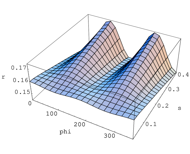
FIG. 1.: The distribution $r(\phi,\hat{s})$ for $(x,u,v)=(0,0,0)$, i.e., $\frac{C_{7R}}{C_{7L}}=0$. This case corresponds to the standard model case. Here $\phi$ is the azimuthal angle between the decay plane of $(K\pi)$ and the decay plane of $(\ell^{+}\ell^{-})$, and $\hat{s}=(p_{\ell^{+}}+p_{\ell^{-}})^{2}/m_{b}^{2}$.

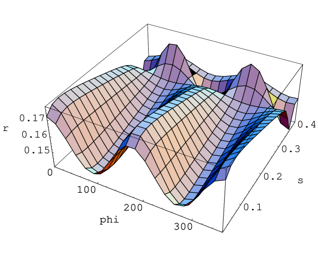
FIG. 2.: The distribution $r(\phi,\hat{s})$ for $(x,u,v)=(\pi/2,0,0)$, i.e., $\frac{C_{7L}}{C_{7R}}=0$.

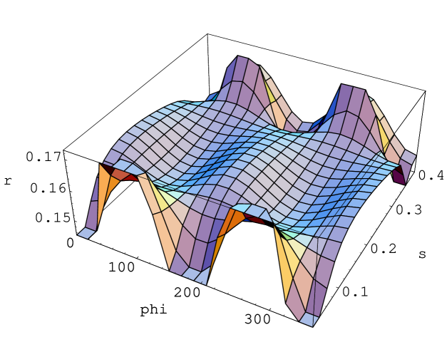
FIG. 3.: The distribution $r(\phi,\hat{s})$ for $(x,u,v)=(\pi/4,0,0)$, i.e., $\frac{C_{7R}}{C_{7L}}=-1$.

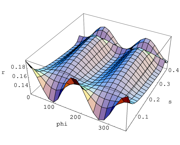
FIG. 4.: The distribution $r(\phi,\hat{s})$ for $(x,u,v)=(-\pi/4,0,0)$, i.e., $\frac{C_{7R}}{C_{7L}}=+1$.

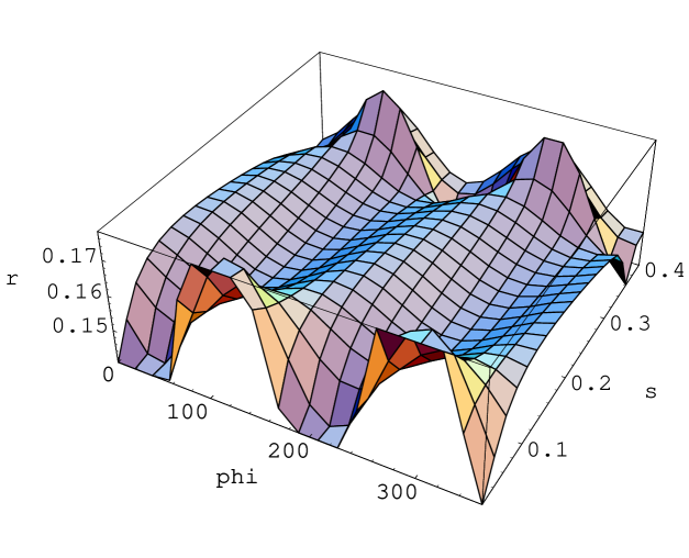
FIG. 5.: The distribution $r(\phi,\hat{s})$ for $(x,u,v)=(\pi/4,0,\pi/8)$, i.e., $\frac{C_{7R}}{C_{7L}}=-\exp(-i\pi/4)$.

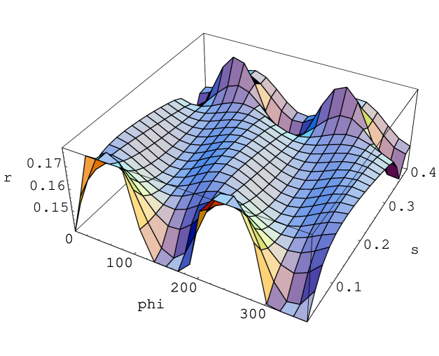
FIG. 6.: The distribution $r(\phi,\hat{s})$ for $(x,u,v)=(\pi/4,0,-\pi/8)$, i.e., $\frac{C_{7R}}{C_{7L}}=-\exp(i\pi/4)$.