Chiral Expansion at Energy Scale of $\rho$-Mass

Abstract

We study chiral expansion at $m_{\rho}$-scale in framework of chiral constituent quark model. The lowest vector meson resonsances are treated as composited fields of constituent quarks. We illustrate that, at energy scale of $\rho$-meson mass, the chiral expansion expansion converges slowly. Therefore, it is possible to construct a well-defined chiral effective field theory at this energy scale, but high order correction of chiral expansion must be included simultanously. The one-loop correction of pseudoscalar mesons is also studied systematically. The unitarity of the model is examined and Breit-Wigner formula for $\rho$-meson is obtained. The prediction on on-shell $\rho\rightarrow\pi\pi$ and $\rho\rightarrow e^{+}e^{-}$ decays agree with data very well.

12.39.-x,12.40.Vv,13.20.Jf,11.15.Pg,13.25.Jx

I Introduction

Although at very low energy the chiral perturbative theory(ChPT)[1] provides an excellent description on interaction of pseudoscalar mesons as well as perturbative QCD works in high energy, it has to be recognized that, so far, we only have a little knowledges concerning underlying dynamical detail at low energy. In particular, in energy region between ChPT($\mu\sim 500$MeV) and chiral symmetry spontaneously broken(CSSB) scale($\Lambda_{\rm CSSB}\sim 1.2$GeV), we do not know how to perform rigorous calculation based on underlying dynamics or symmetry at all, since those well-defined QCD expansion($\alpha_{s}$ expansion, low energy expansion, etc.) converge slowly or even diverge here. Therefore, some phenomenological models(e.g., hidden local symmetry model[2], antisymmetry tensor model[3], WCCWZ model[4]) are constructed for capturing the physics in this energy region. All of these models base on chiral symmetry and only include the lowest order coupling between vector meson resonances and pseudoscalar mesons, i.e., all couplings are momentum-independent and those coupling constants are determined by experiment instead of underlying dynamics. It is obvious that these models only provide very rough physical picture on the lowest vector meson resonances. In general, if a well-defined effective field theory indeed exists at this energy scale, all couplings should be momentum-dependent instead of constants, or these couplings can yield convergence momentum expansion. Since vector meson masses are much larger than pseudoscalar mesons, it is different from ChPT that high order correction of the chiral expansion plays important role here. The purpose of this paper is to provide a possible method to systematically study the chiral expansion at $\rho$-mass scale.

Another fact inspires us to perform this research that the energy scale of CSSB is larger than masses of the lowest vector meson resonances. Therefore, if the chiral expansion is in powers of $p^{2}/\Lambda_{CSSB}^{2}(p\sim m_{\rho})$, it converges slowly. Obviously, in this case contribution from high order terms of momentum expansion plays an important role. However, since we do not know how to derive a low energy effective field theory from QCD directly, we have to construct the low energy effective theory in terms of some approaches with features of low energy QCD. In general, there are two different approaches for studying dynamics of light-flavor $0^{-}$ and $1^{-}$ mesons in framework of effective field theory: One is the method of ChPT, which only needs to assume a certain realization of chiral symmetry for vector mesons(it is standard for symmetry realization of pseudoscalar mesons). The effective lagrangian is written based on these symmetrical reqiurement and is expanded in powers of external momentum. The hidden local symmetry model et. al.[2, 3, 5] belong to this approach. A recent review is in[4]. In principle, this method can be treated as approximate symmetry pattern of QCD and it’s symmetry spontaneously breaking if symmetrical realization of vector mesons is right. Unfortunately, the method of ChPT is impractical here since our calculation in this paper must go beyond the lowest order, and number of free parameters will increase very rapidly. Another approach is method of chiral quark model(ChQM). The Manohar-Georgi(MG) model[7] and Extend Nambu-Jona-Lasinio(ENJL)[8, 9, 10] model et. al. all belong to this approach. In chiral quark model, the vector meson fields are coupling to quark fields. There are no kinetic terms for vector mesons. Therefore they are treated as composited fields of quarks instead of independent degrees of freedom. Effective lagrangian describing dynamics of vector mesons is yielded via quark loop effects. The ChQM approach has some advantages which are try to reflect some underlying dynamical constrains and provide elegant description on some features of low-energy QCD. The main advantage is that number of free parameters does not increase with expansion order rising. So that it is possible to investigate high order correction of momentum expansion systematically. Of course, the ChQM approach is only treated as model instead of rigorous theory, since due to lack of knowledge on QCD low energy behavior, one has to add quark-meson coupling or more undelying four fermion coupling handly according to requirement of symmetry. Although this is a disadvantage of the ChQM approach, the ChQM and its extension[6]-[14] have been studied continually during the last two decades and got great successes in different aspects of phenomenological predictions in hadron physics. In this paper, following spirit shown in MG model, we will construct the chiral constituent quark model(ChCQM) for the lowest vector meson resonances, and provide systematic investigation on dynamics of on-shell $\rho\rightarrow\pi\pi$ and $\rho-e^{+}e^{-}$ decays.

The simplest version of ChQM which was originated by Weinberg[6], and developed by Manohar and Georgi[7] provides a QCD-inspired description on the simple constituent quark model. In view of this model, in the energy region between the CSSB scale and the confinement scale ($\Lambda_{QCD}\sim 0.1-0.3GeV$), the dynamical field degrees of freedom are constituent quarks(quasi-particle of quarks), gluons and Goldstone bosons associated with CSSB(it is well-known that these Goldstone bosons correspond to lowest pseudoscalar octet). In this quasiparticle description, the effective coupling between gluon and quarks is small and the important interaction is the coupling between quarks and Goldstone bosons. Simultaneously, this simple model provide a very rough configuration about baryons, which is baryons can be treated as bound states of three constituent quarks. Thus, from baryon masses, masses of constituent quarks are approximately estimated as 360MeV for u,d flavor and 540MeV for s flavor[7]. We notice that the masses for u,d flavor are very close to $m_{\rho}/2$. In addition, the binding energy of nucleons is expected to be large due to stability of nucleons. It implies that true masses of constituent quarks are larger than our above estimation even $m_{\rho}/2$. Naturally, it is allowed to treat the lowest vector meson resonances as composite fields of constituent quark and antiquarks instead of independent dynamical degree of freedom. Thus, dynamics of vector mesons will be generated by constituent quark loops. This approach is foundation of our study in this paper.

Furthermore, we must point out that, role of pseudoscalar meson fields in constituent quark model is different from other two kinds of ChQM: ENJL model and chiral current quark model[12, 14]. In the latter the pseudoscalar mesons are composited fields of current quark and antiquarks. So that they are not independent dynamical field degree of freedom of these models and dynamics of $0^{-}$ mesons is generated by current quark loops. However, in the former the pseudoscalar mesons are independent dynamics degree of freedom instead of bound states of constituent quarks. This implies that the model is ”part renormalizatable”(for kinetic term of $0^{-}$ mesons). There is no so called double counting problem in this model due to the following two reasons: 1) The constituent quark fields and pseudoscalar mesons(as Goldstone bosons) are generated simultaneously by CSSB. 2) Phenomenologically, the masses of constituent quarks are much larger than of $0^{-}$ mesons. Therefore, if pseudoscalar fields are bound states of constituent quarks, such large binding energy is anti-intuitive. Although ENJL model or chiral current model provide a possibility to probe underly dynamics structure on pseudoscalar mesons, they are failed to touch the goal of this paper, since these models can not yield a sufficient large paramter consistently to make the chiral expansion at energy scale $\mu\sim m_{\rho}$ be convergent.

It has been known that, there are some rather different forms on low energy effective lagrangian including spin-1 meson resonances, and the different types of couplings contained in them. Every approach corresponds to a different chioce of fields for the spin-1 mesons, and they are in principle equivalent. From the viewpoint of chiral symmetry only, an alternative scheme for incorporating spin-1 mesons was suggested by Weinberg[15] and developed further by Callan, Coleman et. al[16]. In this treatment, all spin-1 meson resonances transform homogeneously under a non-linear realizations of chiral $SU(3)$, which are uniquely determined by the known transformation properties under the vectorial subgroup $SU(3)_{V}$(octets and singlet). This is an attractive symmetry property on meson resonances and quite nature in ChCQM, since in this model all dynamical field degree of freedom are associated with CSSB so that lagrangian is explicitly invariant under local $SU(3)_{V}$ transformation. Of course, it is not necessary to describe the degrees of freedom of vector and axial-vector mesons by antisymmetric tensor fields[3], and there are other phenomenological successful attempts to introduce spin-1 meson resonances as massive Yang-Mills fields[2, 12, 17]. We will show that, in ChCQM, vector representation for vector mesons is nature and more convenient than tensor representation.

In past thirties years, various approachs have been attempted to predict hadron phenomenology. Many of these approachs on vector mesons are motivated by phenomenologically successful ideas of vector-meson dominance(VMD) and universal coupling[18, 19]. In ChCQM, we only need start from bound states approachs for vector meson resonances and transformation properties of their vector repsentation. The VMD and universal coupling will be naturally predicted by the model in stead of input. Consequently, other phenomenological relation, such as KSRF sum rules are yielded too. This is anthor advantage of ChCQM. It should be noted that, in making comparisons between ChCQM and other approachs, we need carefully distinguish features coming from the choice of field from those coming from phenomenological requirments. The former are not physical, controlling merely the off-shell behaviour of scattering amplitudes. The later do have physical consequences, such as relations between on-shell amplitudes for different processes. Furthermore, for purpose of this paper, a nature problem appears: Can phenomenological results obtained in leading order still be kept when high order of momentum expansion are considered? This problem will be carelly study in this paper.

It can be known from ChPT, if an effective field theory is constructed in powers of momentum expansion, loop graphs of this field theory which comes from lower order terms will contribute to higher order terms. A nature agruement is loop graphs of effective field theory of QCD are suppressed by $1/N_{c}$ expansion[20]. However, for physical value $N_{c}=3$, this suppression is not suficiently small, so that we can not omit contribution from hadron loop graphs in our calculation(especially, one-loop graph). Due to large mass gap between pseudoscalar mesons and vector meson, it is reasonable assumption that dominant contribution comes from one-loop graphs of pseduoscalar meson. The dynamics including one-loop contribution is very different from one of leading order, for instance, imaginary of ${\cal T}$-matrix of this effective theory will be yielded. Naturally, it is very difficult to deal with ultraviolet(UV) divergence from hadron loops in a framework of non-renormalizable field theory. Fortunately, loop effects of pseudoscalar meson cause $\phi-\omega$ mixing which will destory OZI rule if this contribution is large. Thus we can cancel all UV divergence from $0^{-}$ meson loops in terms of OZI rule.

It is different from some approachs that[3, 9, 12], according to proposition of this paper, physics about axial-vector meson resonances, $a_{1}$(1260), can not be studied here. Since the chiral expansion in this energy region is not convergent. In fact, this problem exists in all approachs including axial-vector meson resonances. Of course, from alternative viewpoint, those approachs can be understood and only be understood as phenomenological models in the leading order. In this paper, since we will provide a rigorous treatment on the chiral expansion, we only focus our attention on vector mesons.

The paper is organized as follows. In sect. 2 the chiral constituent quark model with vector meson resonances are constructed, and the effective lagrangian at leading order are derived. This effective lagranguan is equivalent to WCCWZ lagrangian given by Brise[4]. In sect. 3 we will calculate effective vertices for $\rho-\gamma$ mixing, $\rho\rightarrow\pi\pi$, $\gamma\rightarrow\pi\pi$ and four-pseudoscalar meson coupling. Those effective vertices is generated by constituent quark loops, and include all orders correction of momentum expansion. In sect. 4, one-loop correction generated by pseudoscalar mesons is calculated systematically. Our goal is to estimate hadronic one-loop contribution in $\rho\rightarrow e^{+}e^{-}$ and $\rho\rightarrow\pi\pi$ decay amplitude. The Breit-Wigner formula for $\rho$-propagator is obtained. The unitarity of this effective theory is also examined explicitly. The numerical result is in sect. 5 and sect. 6 is devoted to summary.

II ChCQM with Vector Meson Resonances

A Construction of ChCQM

The QCD lagrangian with three flavour current quark fields $\bar{\psi}=(\bar{u},\bar{d},\bar{s})$ is,

$${\cal L}_{QCD}(x)={\cal L}_{QCD}^{0}+{\cal L}_{\rm f},$$ (2.1)

$${\cal L}_{\rm f}=\bar{\psi}(\gamma\cdot v+\gamma\cdot a\gamma_{5})\psi-\bar{\psi}(s-i\gamma_{5}p)\psi.$$ (2.2)

For our purpose we only pay attention to ${\cal L}_{\rm f}$. Here the fields $v_{\mu},a_{\mu}$ and $p$ are $3\times 3$ matrices in flavour space and denote respectively vector, axial-vector and pseudoscalar external fields. $s={\cal M}+s_{{}_{\rm external}}$, where $s_{{}_{\rm external}}$ is scalar external fields and ${\cal M}$=diag($m_{u},m_{d},m_{s}$) is current quark mass matrix with three flavors.

The introduction of external fields $v_{\mu}$ and $a_{\mu}$ allows for the global symmetry of the lagrangian to be invariant under local $SU(3)_{L}\times SU(3)_{R}$, i.e., with $g_{L},g_{R}\in SU(3)_{L}\times SU(3)_{R}$, the explicit transformations of the different fields are

$$\psi(x)\rightarrow g_{R}(x)\frac{1}{2}(1+\gamma_{5})\psi(x)+g_{L}(x)\frac{1}{2}(1-\gamma_{5})\psi(x),$$ (2.4)

$$l_{\mu}\equiv v_{\mu}-a_{\mu}\rightarrow g_{L}(x)l_{\mu}g_{L}^{\dagger}(x)+ig_{L}(x)\partial_{\mu}g_{L}^{\dagger}(x),$$ (2.5)

$$r_{\mu}\equiv v_{\mu}+a_{\mu}\rightarrow g_{R}(x)r_{\mu}g_{R}^{\dagger}(x)+ig_{R}(x)\partial_{\mu}g_{R}^{\dagger}(x),$$ (2.6)

$$s+ip\rightarrow g_{R}(x)(s+ip)g_{L}^{{\dagger}}(x).$$ (2.7)

Now let energy descend until chiral symmetry is spontanoeusly broken. Below this energy scale, the coupling becomes strong and perturbative QCD can no longer be done, so that we need some effective models(quark model, pole model, Skyrme model…) to approach low energy behaviours of QCD. A successful attempt is achieved by non-linear realization of spontanoeusly broken global chiral symmetry introduced by Weinberg[15]. This realization is obtained by specifying the action of global chiral group $G=SU(3)_{L}\times SU(3)_{R}$ on element $\xi(\Phi)$ of the coset space $G/SU(3)_{{}_{V}}$:

$$\xi(\Phi)\rightarrow g_{R}\xi(\Phi)h^{{\dagger}}(\Phi)=h(\Phi)\xi(\Phi)g_{L}^{{\dagger}},\hskip 72.26999pth(\Phi)\in H=SU(3)_{{}_{V}}.$$ (2.8)

Explicit form of $\xi(\Phi)$ is usually taken

$$\xi(\Phi)=\exp{\{i\lambda^{a}\Phi^{a}(x)/2\}},$$ (2.9)

where the Goldstone boson $\Phi^{a}$ are treated as pseudoscalar meson octet. The compensating $SU(3)_{{}_{V}}$ transformation $h(\Phi)$ defined by Eq.( 2.8) is the wanted ingredent for a non-linear realization of G. In practice, we shall be interested in transformations of constituent quark fields and spin-1 meson resonances under $SU(3)_{{}_{V}}$. The constituent quarks $\bar{q}=(\bar{q}_{u},\bar{q}_{d},\bar{q}_{s})$ are defined as fields whose quantum numbers are same as current quarks $\bar{\psi}$. The $q,\bar{q}$ transform as matter fields of $SU(3)_{{}_{V}}$:

$$q\longrightarrow h(\Phi)q,\hskip 72.26999pt\bar{q}\longrightarrow\bar{q}h^{{\dagger}}(\Phi).$$ (2.10)

The spin-1 meson resonances transform homogeneously as octets and singlets under $SU(3)_{V}$. Denoting the multiplets generically be $O_{\mu}$(octet) and $O_{1\mu}$(singlet), the non-linear realization of G is given by

$${\cal O}_{\mu}\rightarrow h(\Phi){\cal O}_{\mu}h^{{\dagger}}(\Phi),\hskip 72.26999pt{\cal O}_{1\mu}\rightarrow{\cal O}_{1\mu}.$$ (2.11)

More convenience, due to OZI rule, the vector and axial-vector octets and singlets are combined into a single “nonet” matrix

$$N_{\mu}={\cal O}_{\mu}+\frac{I}{\sqrt{3}}{\cal O}_{1\mu},\hskip 57.81621ptN_{\mu}=V_{\mu},A_{\mu},$$

where

$$V_{\mu}(x)={\bf\lambda\cdot V}_{\mu}=\sqrt{2}\left(\begin{array}[]{ccc}\frac{\rho^{0}_{\mu}}{\sqrt{2}}+\frac{\omega_{\mu}}{\sqrt{2}}&\rho^{+}_{\mu}&K^{*+}_{\mu}\\ \rho^{-}_{\mu}&-\frac{\rho^{0}_{\mu}}{\sqrt{2}}+\frac{\omega_{\mu}}{\sqrt{2}}&K^{*0}_{\mu}\\ K^{*-}_{\mu}&\bar{K}^{*0}_{\mu}&\phi_{\mu}\end{array}\right).$$ (2.12)

As momentioned in Introduction, in this formalism we can not study physics at axial-vector meson mass scale consistently, but there is no problem when axial-vector mesons appear as off-shell fields. Thus axial-vector meson resonances $A_{\mu}$ will affect low energy dynamics of pseudoscalar fields through $A_{\mu}-\partial_{\mu}\Phi$ mixing. Therefore we still remain fields $A_{\mu}$ here. But it should be remembered that $A_{\mu}$ only appear as intermediate states, and in this paper we will remove them after we diagonize $A_{\mu}-\partial_{\mu}\Phi$ mixing.

Due to introduction of external fields $v_{\mu}$ and $a_{\mu}$, the model can be extended to be invariant under $G_{\rm glocal}\times G_{\rm local}$. So that it is convenient to put pseudoscalar fields and external vector and axial-vector fields in $SU(3)_{{}_{V}}$ invariant field gradients

$$\Delta_{\mu}=\frac{1}{2}\{\xi^{{\dagger}}(\partial_{\mu}-ir_{\mu})\xi-\xi(\partial_{\mu}-il_{\mu})\xi^{{\dagger}}\},$$ (2.13)

and connection

$$\Gamma_{\mu}=\frac{1}{2}\{\xi^{{\dagger}}(\partial_{\mu}-ir_{\mu})\xi+\xi(\partial_{\mu}-il_{\mu})\xi^{{\dagger}}\}.$$ (2.14)

Under non-linear realization of chiral SU(3) $\Gamma_{\mu}$ transforms as follow:

$$\Gamma_{\mu}\longrightarrow h\Gamma_{\mu}h^{{\dagger}}+h\partial_{\mu}h^{{\dagger}}.$$ (2.15)

Without external fields, $\Gamma_{\mu}$ is the usual natural connection on coset space. Since the above transformation is local we are led to define a covariant derivative

$$d_{\mu}{\cal O}=\partial_{\mu}{\cal O}+[\Gamma_{\mu},{\cal O}],$$ (2.16)

ensuring the proper transformation

$$d_{\mu}{\cal O}\longrightarrow h(\Phi)d_{\mu}{\cal O}h^{{\dagger}}(\Phi).$$ (2.17)

In addition, when we want going beyond chiral limit, the current quark mass enter dynamics by means of the following $SU(3)_{{}_{V}}$ invariant form

$$\frac{1}{4B_{0}}(\xi\chi^{{\dagger}}\xi+\xi^{{\dagger}}\chi\xi^{{\dagger}})+\frac{1}{4B_{0}}\kappa(\xi\chi^{{\dagger}}\xi-\xi^{{\dagger}}\chi\xi^{{\dagger}})\gamma_{5},$$ (2.18)

with $\chi=2B_{0}(s+ip)$.

By using on similar discussion, Manahor and Georgi provide a simple pattern of ChCQM for understanding the physics between CSSB scale and quark confinement scale[7]. The MG model are described by the following chiral constituent quark lagrangian

$${\cal L}_{\rm MG}=i\bar{q}\gamma\cdot(\partial+\Gamma+g_{{}_{A}}\Delta\gamma_{5})q-m\bar{q}q+\frac{F^{2}}{16}<\nabla_{\mu}U\nabla^{\mu}U^{{\dagger}}>,$$ (2.19)

where $U(\Phi)=\xi^{2}(\Phi)$, $g_{{}_{A}}$ is coupling constant of axial-vector current whose value $g_{{}_{A}}\simeq 0.75$ can be fitted by $n\rightarrow pe^{-}\bar{\nu}_{e}$ decay. The $<...>$ denotes trace in SU(3) flavour space and covariant derivative is defined as follows:

$$\nabla_{\mu}U = \partial_{\mu}U-ir_{\mu}U+iUl_{\mu}=2\xi\Delta_{\mu}\xi,$$ (2.20)

$$\nabla_{\mu}U^{{\dagger}} = \partial_{\mu}U^{{\dagger}}-il_{\mu}U^{{\dagger}}+iU^{{\dagger}}r_{\mu}=-2\xi^{{\dagger}}\Delta_{\mu}\xi^{{\dagger}}.$$ (2.21)

In lagrangian( 2.19), mass of constituent quarks $m$ is a paramter relating to CSSB. Here we treat that mass difference of constituent quarks for different flavors are caused by current quark masses. According to the discussions presented in the Introduction, it is theoretically self-consistent when kinetic term of pseudoscalar mesons is introduced initially. Thus MG model is renormalizable for kinetic term and the lowest order interaction term of pseudoscalar meson. The high order interaction for $0^{-}$ mesons will be generated by both of loop effects of quarks and loop effects of the lowest order interaction of mesons. By means of M-G model, the quark mass-independent low energy coupling constants have been derived in Refs.[13, 21]. It is remarkable that the predictions of this simple model are in agreement with the phenomenological values of $L_{i}$ in ChPT. This means the low energy limit M-G model is compatible with ChPT in chiral limit. In the baryon physics, the skyrmion calculations show also that the predictions from M-G model are reasonable[11, 22, 23].

This simple model provides an useful description on physics between CSSB scale ($\mu\sim 1.2$GeV) and quark confinement scale ($\mu\sim 0.1-0.3$GeV). That is if we live in a world with this energy region only, perhaps we will not think about what is quark confinement very much, or even can not discover what QCD is at all. We can construct a consistent “field theory” in terms of Goldstone bosons and those “fake element particles”-constituent quarks. We will be perfectly satisfied with perturbative theory of this ”field theory”. Now let us return from these philosophical discussiones. It should be remembered constituent quark is only virtual field here. In real world, its kinetic degree of freedom is contained by its composited states, e.g., the lowest order meson resonances and nucleon. Since scalar octet and singlet of chiral SU(3) are not confirmed by experiment, we will ignore them in this paper.

According to provious discussion on spin-1 meson resonances, the MG model is easily to extended to include spin-1 meson resonances,

$${\cal L}_{\chi} = i\bar{q}\gamma\cdot(\partial+\Gamma+\tilde{g}_{{}_{A}}\Delta\gamma_{5})q+\bar{q}\gamma\cdot(V+A\gamma_{5})q-m\bar{q}q-\frac{1}{4B_{0}}\bar{q}(\xi\chi^{{\dagger}}\xi+\xi^{{\dagger}}\chi\xi^{{\dagger}})q$$ (2.23)

$$-\frac{1}{4B_{0}}\kappa\bar{q}(\xi\chi^{{\dagger}}\xi-\xi^{{\dagger}}\chi\xi^{{\dagger}})\gamma_{5}q+\frac{F^{2}}{16}<\nabla_{\mu}U\nabla^{\mu}U^{{\dagger}}>+\frac{1}{4}m_{0}^{2}<V_{\mu}V^{\mu}+A_{\mu}A^{\mu}>.$$

Although we have introduced current quark mass in lagrangian ( 2.23), the pseudoscalar fields are still massless since they are GoldStone bosons associated CSSB. The masses of pseudoscalar mesons are generated via loop effects of constituent quarks. In addition, $A_{\mu}-\partial^{\mu}\Phi$ mixing are also caused by constituent quark loops. The symmetry requires this mixing to appear according to form $<A_{\mu}\Delta^{\mu}>$. Thus this mixing can be diagnolized via field shift

$$A_{\mu}\longrightarrow A_{\mu}-ic\Delta_{\mu}.$$ (2.24)

This field shift is nothing but to modify axial-vector current coupling constant $\tilde{g}_{{}_{A}}$ in Eq.( 2.23), i.e., $g_{{}_{A}}=\tilde{g}_{{}_{A}}-c$. Recalling axial-vector meson resonances appear only as intermediate states, therefore, in fact, we can get rid of axial-vector meson fields in lagrangian ( 2.23) and chiral lagrangian ( 2.23) is rewirtten

$${\cal L}_{\chi} = i\bar{q}\gamma\cdot(\partial+\Gamma+g_{{}_{A}}\Delta\gamma_{5}-iV)q-m\bar{q}q-\frac{1}{4B_{0}}\bar{q}(\xi\chi^{{\dagger}}\xi+\xi^{{\dagger}}\chi\xi^{{\dagger}})q$$ (2.26)

$$-\frac{1}{4B_{0}}\kappa\bar{q}(\xi\chi^{{\dagger}}\xi-\xi^{{\dagger}}\chi\xi^{{\dagger}})\gamma_{5}q+\frac{F^{2}}{16}<\nabla_{\mu}U\nabla^{\mu}U^{{\dagger}}>+\frac{1}{4}m_{0}^{2}<V_{\mu}V^{\mu}>.$$

Here it should be rememberd that the experimental value $g_{{}_{A}}\simeq 0.75$ has included the effect of $A_{\mu}-\partial^{\mu}\Phi$ mixing.

B Effective lagrangian

In this subsection, we like to derive the lowest order effective lagrangian describing the coupling between vector meson resonances and pseudoscalar mesons.

A review for chiral gauge theory is in [24]. The effective lagrangian of mesons in ChQM can be obtained in Euclidian space by means of integrating over degrees of freedom of fermions in lagrangian( 2.26)

$$\exp\{-\int d^{4}x{\cal L}_{eff}\}=\int{\cal D}\bar{q}{\cal D}q\exp\{-\int d^{4}x{\cal L}_{\chi}\}.$$ (2.27)

Then we have

$${\cal L}_{eff}=-\ln{\rm det}{\cal D},$$ (2.28)

with

$${\cal D}=\gamma^{\mu}(\partial_{\mu}+\Gamma_{\mu}+g_{A}\Delta_{\mu}\gamma_{5}-iV_{\mu})+m-\frac{1}{4B_{0}}(\xi\chi^{{\dagger}}\xi+\xi^{{\dagger}}\chi\xi^{{\dagger}})-\frac{1}{4B_{0}}\kappa(\xi\chi^{{\dagger}}\xi-\xi^{{\dagger}}\chi\xi^{{\dagger}})\gamma_{5}.$$ (2.29)

The effective lagrangian is separated into two parts

$${\cal L}_{eff}={\cal L}_{eff}^{Re}+{\cal L}_{eff}^{Im}$$ (2.30)

$${\cal L}_{eff}^{Re}=-\frac{1}{2}\ln{\rm det}({\cal D}{\cal D}^{{\dagger}}),\hskip 57.81621pt{\cal L}_{eff}^{Im}=-\frac{1}{2}\ln{\rm det}[({\cal D}^{{\dagger}})^{-1}{\cal D}]$$ (2.31)

where

$${\cal D}^{{\dagger}}=\gamma_{5}\hat{{\cal D}}\gamma_{5},$$ (2.32)

and $\hat{B}=\frac{1}{2}(1+\gamma_{5})B_{L}+\frac{1}{2}(1-\gamma_{5})B_{R}$ for arbitrarily operator $B=\frac{1}{2}(1-\gamma_{5})B_{L}+\frac{1}{2}(1+\gamma_{5})B_{R}$. The effective lagrangian ${\cal L}_{eff}^{Re}$ describes the physical processes with normal parity and ${\cal L}_{eff}^{Im}$ the processes with anomal parity. In the present paper we focus our attention on ${\cal L}_{eff}^{Re}$. The discussion of ${\cal L}_{eff}^{Im}$ can be found in Refs.[24, 12]. In terms of Schwenger’s proper time method [25], ${\cal L}_{eff}^{Re}$ is written as

$${\cal L}_{eff}^{Re}=-\frac{1}{2\delta(0)}\int d^{4}x\frac{d^{4}p}{(2\pi)^{4}}Tr\int_{0}^{\infty}\frac{d\tau}{\tau}(e^{-\tau{\cal D}^{\prime\dagger}{\cal D}^{\prime}}-e^{-\tau\Delta_{0}})\delta^{4}(x-y)|_{y\rightarrow x}$$ (2.33)

with

$${\cal D}^{\prime}={\cal D}-i\gamma\cdot p,\hskip 57.81621pt{\cal D}^{\prime{\dagger}}={\cal D}^{{\dagger}}+i\gamma\cdot p,$$ (2.34)

$$\Delta_{0}=p^{2}+M^{2}.$$ (2.35)

where M is an arbitrary parameter with dimension of mass. The Seeley-DeWitt coefficients or heat kernel method have been used to evaluate the expansion series of Eq.( 2.34). In this paper we will use dimensional regularization. After completing the integration over $\tau$, the lagrangian ${\cal L}_{eff}^{Re}$ reads

$${\cal L}_{eff}^{Re}=-\frac{\mu^{\epsilon}}{2\delta(0)}\int d^{D}x\frac{d^{D}p}{(2\pi)^{D}}\sum_{i=1}^{\infty}\frac{1}{n\Delta_{0}^{n}}Tr({\cal D}^{\prime\dagger}{\cal D}^{\prime}-\Delta_{0})^{n}\delta^{D}(x-y)|_{y\rightarrow x},$$ (2.36)

where trace is taken over the color, flavor and Lorentz space. This effective lagrangian can be expanded in powers of derivatives,

$${\cal L}_{Re}={\cal L}_{2}+{\cal L}_{4}+....$$ (2.37)

At order $p^{2}$, we will encounter logarithmic and quadratic divergences in effective lagrangian generated by quark loops. The logarithmic divergence can be canceled via renormalization of kinetic term of pseudoscalar mesons. However, the quadratic divergence can not be renormalized. Thus we need to define a constant $B_{0}$ to factorize the quadratic divergence(or equivalently, to introduce a cut-off to truncate the divergence). Explicitly, ${\cal L}_{2}$ reads

$${\cal L}_{2}=\frac{F_{0}^{2}}{16}<\nabla_{\mu}U\nabla^{\mu}U^{{\dagger}}+\chi U^{{\dagger}}+U\chi^{{\dagger}}>+\frac{1}{4}m_{0}^{2}<V_{\mu}V^{\mu}>,$$ (2.38)

where

$$\frac{F_{0}^{2}}{16} = \frac{F^{2}}{16}+\frac{N_{c}}{(4\pi)^{D/2}}(\frac{\mu^{2}}{m^{2}})^{\epsilon/2}\Gamma(2-\frac{D}{2})g_{A}^{2}m^{2},$$ (2.39)

$$\frac{F_{0}^{2}}{16}B_{0} = \frac{N_{c}}{(4\pi)^{D/2}}(\frac{\mu^{2}}{m^{2}})^{\epsilon/2}\Gamma(1-\frac{D}{2})m^{3}.$$ (2.40)

In chiral limit, it is known that $F_{0}$ just is decay constants of $\pi$ mesons, $F_{0}=f_{\pi}=185$MeV. The lagrangian ( 2.38) yields equation of motion of pseudoscalar mesons

$$\nabla_{\mu}(U\nabla^{\mu}U^{{\dagger}})+\frac{1}{2}(\chi U^{{\dagger}}-U\chi^{{\dagger}})=0.$$ (2.41)

Up to order $p^{4}$, all pseudoscalar meson fields satisfy this equation.

At order $p^{4}$ the effective lagrangian generated by quark loops reads

$${\cal L}_{4}^{(q)} = -[\frac{g^{2}}{8}-\frac{\gamma}{12}]<L_{\mu\nu}L^{\mu\nu}+R_{\mu\nu}R^{\mu\nu}>-\frac{\gamma}{6}<L_{\mu\nu}R^{\mu\nu}>$$ (2.44)

$$-\frac{i\gamma}{3}g_{A}^{2}<\nabla_{\mu}U\nabla_{\nu}U^{{\dagger}}\xi R^{\mu\nu}\xi^{{\dagger}}+\nabla_{\mu}U^{{\dagger}}\nabla_{\nu}U\xi^{{\dagger}}L^{\mu\nu}\xi>+\frac{\gamma}{12}g_{A}^{4}<\nabla_{\mu}U\nabla_{\nu}U^{{\dagger}}\nabla^{\mu}U\nabla^{\nu}U^{{\dagger}}>$$

$$+\theta_{1}g_{A}^{2}<\nabla_{\mu}U\nabla^{\mu}U^{{\dagger}}(\chi U^{{\dagger}}+\chi^{{\dagger}}U)>+\theta_{2}<\chi U^{{\dagger}}\chi U^{{\dagger}}+\chi^{{\dagger}}U\chi^{{\dagger}}U>$$

where

$$\frac{3}{8}g^{2} = \frac{N_{c}}{(4\pi)^{D/2}}(\frac{\mu^{2}}{m^{2}})^{\epsilon/2}\Gamma(2-\frac{D}{2}),\hskip 36.135pt\gamma=\frac{N_{c}}{(4\pi)^{2}},\hskip 36.135pt\theta_{1}=(\frac{3}{8}g^{2}-\gamma)\frac{m}{2B_{0}},$$ (2.45)

$$\theta_{2} = \frac{F_{0}^{2}}{128B_{0}m}(3-\kappa^{2})+\frac{3m}{64B_{0}}g^{2}(\frac{m}{B_{0}}-\kappa g_{{}_{A}}+\frac{g_{{}_{A}}^{2}}{2})-\frac{\gamma}{24}g_{A}^{2},$$ (2.46)

$$L_{\mu\nu} = \frac{1}{2}(1+g_{A})\xi F_{\mu\nu}^{L}\xi^{{\dagger}}+\frac{1}{2}(1-g_{A})\xi^{{\dagger}}F_{\mu\nu}^{R}\xi+V_{\mu\nu}-i(1-g_{A}^{2})[\Delta_{\mu},\Delta_{\nu}]-g_{A}([\Delta_{\mu},V_{\nu}]+[V_{\mu},\Delta_{\nu}]),$$ (2.47)

$$R_{\mu\nu} = \frac{1}{2}(1+g_{A})\xi^{{\dagger}}F_{\mu\nu}^{R}\xi+\frac{1}{2}(1-g_{A})\xi F_{\mu\nu}^{L}\xi^{{\dagger}}+V_{\mu\nu}-i(1-g_{A}^{2})[\Delta_{\mu},\Delta_{\nu}]+g_{A}([\Delta_{\mu},V_{\nu}]+[V_{\mu},\Delta_{\nu}]),$$ (2.48)

with

$$F_{\mu\nu}^{R.L} = \partial_{\mu}(v_{\nu}\pm a_{\nu})-\partial_{\mu}(v_{\nu}\pm a_{\nu})-i[v_{\mu}\pm a_{\mu},v_{\nu}\pm a_{\nu}].$$ (2.49)

$$V_{\mu\nu} = d_{\mu}V_{\nu}-d_{\nu}V_{\mu}-i[V_{\mu},V_{\nu}].$$ (2.50)

Here an universal coupling constant $g$ of the effective field theory absorbs logarithmic divergences in Eq. (2.44).

From the kinetic terms of meson fields in lagrangians ( 2.38) and ( 2.44) we can see that meson fields are not physical. The physical meson fields can be defined via the following field rescaling in effective lagrangian which make the kinetic terms of meson fields into the standard form

$$V_{\mu}\longrightarrow\frac{1}{g}V_{\mu},\hskip 72.26999pt\Phi\longrightarrow\frac{2}{f_{\Phi}}\Phi.$$ (2.51)

where $\Phi=\pi,\;K,\;\eta$.

C Vector meson dominant and KSRF sum rules

The direct coupling between photon and vector meson resonances is also yielded by the effects of quark loops. Therefore, if vector meson resonances are treated as bound states of constituent quarks, vector meson dominant will be yielded naturally instead of input. At isovector channel it reads from lagrangian ( 2.44)

$${\cal L}_{\rho\gamma}=-\frac{1}{4}eg(\partial^{\mu}{\cal A}^{\nu}-\partial^{\nu}{\cal A}^{\mu})(\partial_{\mu}\rho_{\nu}^{0}-\partial_{\nu}\rho_{\mu}^{0}),$$ (2.52)

where ${\cal A}_{\mu}$ is photon fields. Above equation is just the expression of VMD proposed by Sakurai[18]. Similarly, at isoscalar channel they read

$${\cal L}_{\omega\gamma} = -\frac{1}{12}eg(\partial^{\mu}{\cal A}^{\nu}-\partial^{\nu}{\cal A}^{\mu})(\partial_{\mu}\omega_{\nu}-\partial_{\nu}\omega_{\mu}),$$ (2.53)

$${\cal L}_{\phi\gamma} = \frac{1}{6}eg(\partial^{\mu}{\cal A}^{\nu}-\partial^{\nu}{\cal A}^{\mu})(\partial_{\mu}\phi_{\nu}-\partial_{\nu}\phi_{\mu}).$$ (2.54)

It is well known that the KSRF(I) sum rule[26]

$$g_{\rho\gamma}(q^{2})=\frac{1}{2}f_{\rho\pi\pi}(q^{2})f_{\pi}^{2}$$ (2.55)

is the result of current algebra and PCAC. So that it is expected to be available at the leading order of momentum expansion. The $g_{\rho\gamma}(q^{2})$ is obtained from experssion ( 2.52)

$$g_{\rho\gamma}(q^{2})=\frac{1}{2}gq^{2}$$ (2.56)

In addition, if we set $m_{u}=m_{d}=0$, the lowest order $\rho\rightarrow\pi\pi$ vertex reads

$${\cal L}_{\rho\pi\pi} = f_{\rho\pi\pi}(q^{2})\epsilon^{ijk}\rho_{i}^{\mu}\pi_{j}\partial_{\mu}\pi_{k},$$ (2.57)

$$f_{\rho\pi\pi}(q^{2}) = \frac{q^{2}}{gf_{\pi}^{2}}[g^{2}-(g^{2}-\frac{N_{c}}{3\pi^{2}})g_{A}^{2}].$$ (2.58)

From Eqs. (2.56) and (2.57) we can find that $g=\sqrt{\frac{N_{c}}{3}}\frac{1}{\pi}$ satisfy KSRF(I) sum rule exactly. Therefore, $g\equiv\sqrt{\frac{N_{c}}{3}}\frac{1}{\pi}$ (especially, $g\equiv\pi^{-1}$ for $N_{c}=3$) is favorite choice for the universal constant of the model.

The interaction of vector meson resonances in the effective lagrangian (2.44) is similar to WCCWZ lagrangian given by Brise[4]. It is of an expected result since the symmetry realization of vector mesons in our model is the same as one in WCCWZ approch. In addition, those phenomenological requirements, such as VMD and univesal coupling are also satisfied in this lowest order effective lagrangian. It implies that ChCQM is legitimate approch on vector meson resonances. However, the above $f_{\rho\pi\pi}(m_{\rho}^{2})$ and $g_{\rho\gamma}(m_{\rho}^{2})$ yield that the widths of two on-shell decays are $\Gamma(\rho\rightarrow\pi\pi)=125$MeV and $\Gamma(\rho\rightarrow e^{+}e^{-})=4.35$KeV. Comparing with experiment data, the error bars of those theoretical widths are about $15\%$ and $35\%$ respectively. It can be naturally understood since the contributions from high order terms of momentum expansion are droped here. Thus we expect that these droped contributions could make the theoretical prediction close to data.

D Low energy limit

It is well known that, at very low energy, ChPT is a rigorous consequence of the symmetry pattern of QCD and its spontaneous breaking. So that the low energy limit of ChCQM must match with ChPT. The low energy limit of this model can be obtained via integrating over vector meson resonances. It means that, at very low energy, the dynamics of vector mesons are replaced by pseudoscalar meson fields. Since there are no interaction of vector mesons in ${\cal L}_{2}$, at very low energy, the equation of motion $\delta{\cal L}/\delta V_{\mu}=0$ yields classics solution for vector mesons are follow

$$V_{\mu}=\frac{1}{m_{{}_{V}}^{2}}\times O(p^{3}){\rm terms},$$ (2.59)

where $p$ is momentum of pseudoscalar at very low energy. Therefore, in lagrangian ( 2.44), the terms involving vector meson resonances are $O(p^{6})$ at very low energy and do not contribute to $O(p^{4})$ low energy coupling constants, $L_{i}(i=1,2,...,10)$. The low energy coupling constants yielded by ChCQM(besides of $L_{7}$) can be directly obtained from lagrangian (2.44)

$$L_{1} = \frac{1}{2}L_{2}=\frac{\gamma}{24},\hskip 57.81621ptL_{3}=-\frac{\gamma}{4}+\frac{\gamma}{12}g_{A}^{4},$$ (2.60)

$$L_{4} = L_{6}=0,\hskip 72.26999ptL_{5}=\frac{\gamma m}{2B_{0}}g_{A}^{2}$$ (2.61)

$$L_{8} = \frac{F_{0}^{2}}{128B_{0}m}(3-\kappa^{2})+\frac{3m}{64\pi^{2}B_{0}}(\frac{m}{B_{0}}-\kappa g_{{}_{A}}+\frac{g_{{}_{A}}^{2}}{2})-\frac{1}{128\pi^{2}}g_{A}^{2},$$ (2.62)

$$L_{9} = \frac{\gamma}{3},\hskip 97.56493ptL_{10}=-\frac{\gamma}{3}+\frac{\gamma}{6}g_{A}^{2}.$$ (2.63)

The constants $L_{7}$ has been known to get dominant contribution from $\eta_{0}$[1] and this contribution is suppressed by $1/N_{c}$. If we ignore the $\eta-\eta^{\prime}$ mixing, we have

$$L_{7}=-\frac{f_{\pi}^{2}}{128m_{\eta^{\prime}}^{2}}.$$ (2.64)

Thus the five free parameters, $g$(it has been fitted by KSRF sum rule), $g_{{}_{A}}$(it has been fitted by $n\rightarrow pe^{-}\bar{\nu}_{e}$ decay), $\kappa$, $m$ and $m_{\eta^{\prime}}$ determine all ten low energy coupling constants of ChPT. It reflects the dynamics constraints between those low energy coupling constants. Here if we take $m_{u}+m_{d}\simeq 10$MeV, we can obtain $B_{0}=\frac{m_{\pi}^{2}}{m_{u}+m_{d}}\simeq 2$GeV. Inputting experimental values of $L_{5}$ and $L_{8}$, we obtain $m\simeq 480$MeV and $\kappa\simeq 0.2$. The numerical results for these low energy constants are in table 1. We can find that all of them agree with experimental data well. Here the constituent quark mass $m>m_{\rho}/2$, which is the same as out expectation. In next section we will see that it is a necessary condition for yielding a convergence expansion at $\rho$ mass scale.

	$L_{1}$	$L_{2}$	$L_{3}$	$L_{4}$	$L_{5}$	$L_{6}$	$L_{7}$	$L_{8}$	$L_{9}$	$L_{10}$
ChPT	$0.7\pm 0.3$	$1.3\pm 0.7$	$-4.4\pm 2.5$	$-0.3\pm 0.5$	$1.4\pm 0.5$	$-0.2\pm 0.3$	$-0.4\pm 0.15$	$0.9\pm 0.3$	$6.9\pm 0.7$	$-5.2\pm 0.3$
ChCQM	0.79	1.58	-4.25	0	$1.4^{a)}$	0	$(-0.4\pm 0.1)^{b)}$	$0.9^{a)}$	6.33	-4.55

TABLE I.: $L_{i}$ in units of $10^{-3}$, ${\mu}=m_{\rho}$. a)input. b)contribution from gluon anomaly.

III Diagram Analysis and Chiral Expansion at $\rho$ Mass Scale

In previous section, we have derived the leading order effective lagrangian of mesons via integrating out constituent quark fields in original lagrangian. This path integral analysis is equivalent to calculate the one-loop contribution of constituent quarks. The advantage of path integral method is that we can derive an united effective lagrangian of mesons, which is invariant under chiral transformation for every orders of momentum expansion. However, it is disadvantage of path integral method that it is hard to calculate high order contribution of momentum expansion. This shortage can be compensated through calculating one-loop graphs of constituent quarks directly. In this section we will derive effective vertices for $\gamma\rightarrow\pi\pi$, $\rho\rightarrow\pi\pi$, 4-pseudoscalar mesons and $\rho-\gamma$ coupling via diagram analysis. All calculations will be performed at chiral limit.

We start with lagrangian( 2.26). The effective action can be obtained via integrating over degrees of freedom of fermions,

$$e^{iS_{\rm eff}}\equiv\int{\cal D}\bar{q}{\cal D}qe^{i\int d^{4}x{\cal L}_{\chi}(x)}=<vac,out|in,vac>^{V,\Gamma,\Delta},$$ (3.1)

where $<vac,out|in,vac>^{V,\Gamma,\Delta}$ is vacuum expectation value in presence of external source $V_{\mu}$, $\Gamma_{\mu}$ and $\Delta_{\mu}$. In interaction picture, the above equation is rewritten as follow

$$e^{iS_{\rm eff}} = <0|{\cal T}_{q}e^{i\int d^{4}x{\cal L}^{\rm I}_{\chi}(x)}|0>$$ (3.2)

$$= \sum_{n=1}^{\infty}i\int d^{4}p_{1}\frac{d^{4}p_{2}}{(2\pi)^{4}}\cdots\frac{d^{4}p_{n}}{(2\pi)^{4}}\tilde{\Pi}_{n}(p_{1},\cdots,p_{n})\delta^{4}(p_{1}-p_{2}-\cdots-p_{n})$$ (3.3)

$$\equiv i\Pi_{1}(0)+\sum_{n=2}^{\infty}i\int\frac{d^{4}p_{1}}{(2\pi)^{4}}\cdots\frac{d^{4}p_{n-1}}{(2\pi)^{4}}\Pi_{n}(p_{1},\cdots,p_{n-1}),$$ (3.4)

where ${\cal T}_{q}$ is time-order product of constituent quark fields, ${\cal L}_{\chi}^{\rm I}$ is interaction part of lagrangian( 2.26), $\tilde{\Pi}_{n}(p_{1},\cdots,p_{n})$ is one-loop effects of constituent quarks with $n$ external sources(hereafter we call it as $n$-point effective vertex in momentum space), $p_{1},p_{2},\cdots,p_{n}$ are momentums of n external sources respectively and

$$\Pi_{n}(p_{1},\cdots,p_{n-1})=\int d^{4}p_{n}\tilde{\Pi}_{n}(p_{1},\cdots,p_{n})\delta^{4}(p_{1}-p_{2}-\cdots-p_{n}).$$ (3.5)

To get rid of all disconnected diagrams, we have

$$S_{\rm eff} = \int d^{4}x{\cal L}_{\rm eff}(x)=\Pi_{1}(0)+\sum_{n=2}^{\infty}\int\frac{d^{4}p_{1}}{(2\pi)^{4}}\cdots\frac{d^{4}p_{n-1}}{(2\pi)^{4}}\Pi_{n}(p_{1},\cdots,p_{n-1})$$ (3.6)

$$\Rightarrow {\cal L}_{\rm eff}(x)=\sum_{n=1}^{\infty}\int d^{4}p_{1}\frac{d^{4}p_{2}}{(2\pi)^{4}}\cdots\frac{d^{4}p_{n}}{(2\pi)^{4}}e^{i(p_{1}-p_{2}-\cdots-p_{n})\cdot x}\tilde{\Pi}_{n}(p_{1},\cdots,p_{n}).$$ (3.7)

A Two-point effective vertex

There is no tapole diagram contribution of fermions, i.e., $\Pi_{1}(0)\equiv 0$. Thus we start calculating two-point effective vertex $\Pi_{2}(p)$ generated by fermion loop in figure(3.1). Due to parity conservation, here both of two external sources are vector external sources $(V_{\mu}+i\Gamma_{\mu})$, or axial-vector external sources $g_{A}\Delta_{\mu}$.

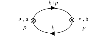
FIG. 3.1.: Two-point effective vertex generated by constituent quark one-loop, where $p$ is external momentum and $k$ is momentum of interal lines.

Employing the completeness relation of generators $\lambda^{a}(a=1,2,...,N^{2}-1)$ of SU(N) group

$$<\lambda^{a}A\lambda^{a}B>=-\frac{2}{N}<AB>+2<A><B>,$$ (3.8)

$$<\lambda^{a}A><\lambda^{a}B>=2<AB>-\frac{2}{N}<A><B>,$$ (3.9)

the two-point effective action is easily to obtain

$$S_{2} = \frac{f_{\pi}^{2}}{16}\int d^{4}x<\nabla_{\mu}U\nabla^{\mu}U^{{\dagger}}>$$ (3.11)

$$-\int\frac{d^{4}p}{(2\pi)^{4}}\frac{A(p^{2})}{4}(\delta_{\mu\nu}p^{2}-p_{\mu}p_{\nu})<(V^{\mu}(p)+i\Gamma^{\mu}(p))(V^{\nu}(-p)+i\Gamma^{\nu}(-p))>,$$

where

$$A(p^{2})\equiv g^{2}-\frac{N_{c}}{\pi^{2}}\int_{0}^{1}dx\cdot x(1-x)\ln{(1-\frac{x(1-x)p^{2}}{m^{2}})}.$$ (3.12)

From Eq.( 3.12) we can see that unitarity of the effective theory requires $4m^{2}>p^{2}$. This requirement also ensures that the momentum expansion is convergent. Here we must point out that we can not work in chiral limit simply if we want to study on-shell $K^{*}(892)$ physics or on-shell $\phi(1020)$ physics. The reason is that $4m^{2}>p^{2}\sim m_{\rho}^{2}$ can not ensure $4m^{2}>p^{2}\sim m_{K^{*}}^{2}$ or $4m^{2}>p^{2}\sim m_{\phi}^{2}$. If we set $m_{u}=m_{d}=0$ but $m_{s}\neq 0$, the unitarity and convergence of momentum expansion require that $4m(m+m_{s})>p^{2}$ for $p^{2}\simeq m_{K^{*}}^{2}$, and $4(m+m_{s})^{2}>p^{2}$ for $p^{2}\simeq m_{\phi}^{2}$. Those requirements are satisfied indeed for $4m^{2}>m_{\rho}^{2}$ and usual value of strange quark mass, i.e., $m_{s}\sim 150$MeV. Therefore, strange quark mass can not be omitted when we study chiral expansion in $m_{{}_{K^{*}}}$ or $m_{\phi}$ scale. In this paper, since we work in $\rho$-meson scale, chiral limit is a good approximation.

In the following, we derive those effective vertices from Eq.( 3.11) which relate to the purposes of this paper. The free field lagrangian of $\rho$-meson reads

$${\cal L}_{\rm kin}^{(\rho)}=-\frac{1}{4}\rho_{\mu\nu}^{i}\rho^{i\mu\nu}+\frac{1}{2}m_{\rho}^{2}\rho_{\mu}^{i}\rho^{i\mu}.$$ (3.13)

where $\rho_{\mu\nu}^{i}=(\partial_{\mu}\rho_{\nu}^{i}-\partial_{\nu}\rho_{\mu}^{i})$. The above lagrangian yields the classic equation of motion of $\rho$-meson in momentum space as follow

$$\frac{1}{2}(p^{2}\delta_{\mu\nu}-p_{\mu}p_{\nu}-m_{\rho}^{2}\delta_{\mu\nu})\rho^{\mu}=0$$ (3.14)

Since in the present paper, all $\rho$-fields are treated at tree level, they should obey the above equation of motion.

The two-point vertex $\rho$-meson reads

$${\cal L}_{\rho\rho}=-\frac{1}{4}[\frac{A(p^{2})}{g^{2}}-1]\rho_{\mu\nu}^{i}\rho^{i\mu\nu},$$ (3.15)

where $p^{2}$ defined by $p^{2}\rho_{\nu}=-\partial^{2}\rho_{\nu}$ is operator in coordinate space. Using this equation of motion in Eq.( 3.14), we have

$$m_{\rho}^{2}=\frac{m_{0}^{2}}{g^{2}}+\frac{N_{c}}{\pi^{2}g^{2}}m_{\rho}^{2}\int_{0}^{1}dx\cdot x(1-x)\ln{(1-\frac{x(1-x)m_{\rho}^{2}}{m^{2}})}.$$ (3.16)

The experimental data $m_{\rho}=770$MeV yields $m_{0}=288$MeV.

The effective vertex describing $\rho-\gamma$ coupling reads

$${\cal L}_{\rho\gamma}=-\frac{1}{8}A(p^{2})<\rho_{\mu\nu}(\xi\gamma^{\mu\nu}\xi^{{\dagger}}+\xi^{{\dagger}}\gamma^{\mu\nu}\xi)>,$$ (3.17)

where

$$\gamma_{\mu\nu}=e{\cal Q}(\partial_{\mu}{\cal A}_{\nu}-\partial_{\nu}{\cal A}_{\mu}),$$ (3.18)

with ${\cal Q}={\rm diag}\{2/3,-1/3,-1/3\}$ is charge operator of quark fields. Comparing effective vertices ( 3.17) with leading order effective lagrangian ( 2.44), we can see that the couplings in Eqs.( 3.17) is momentum-dependent.

B Contribution of triangle diagram

There are two triangle diagrams(figure (3.2)) which also concern the 4-pseudoscalar meson, $\gamma\rightarrow\varphi\varphi$ and $\rho\rightarrow\varphi\varphi$ vertices. The calculation on figure (3.2) is well-known,

$$\Pi_{3}(p,q)=-\frac{1}{2}g_{A}^{2}B(p^{2})p^{\mu}<(V_{\nu}(p)+i\Gamma_{\nu}(p))[\Delta_{\mu}(p-q),\Delta_{\nu}(q)]>,$$ (3.19)

where

$$B(p^{2})=-g^{2}+\frac{N_{c}}{2\pi^{2}}\int_{0}^{1}dx\cdot x\int_{0}^{1}dy(1-xy)[1+\frac{m^{2}}{m^{2}-f(p^{2})}+\ln{(1-\frac{f(p^{2})}{m^{2}})}],$$ (3.20)

where $g^{2}$ absorbes the logarithmic divergence from loop integral, and $f(p^{2})=x(1-x)(1-y)p^{2}$.

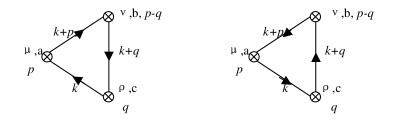
FIG. 3.2.: The triangle diagrams relate to $\gamma\rightarrow\varphi\varphi$ and $\rho\rightarrow\varphi\varphi$, where $p$ is external momentum of vector current, $q$ is external momentum of axial-vector current and $k$ is momentum of interal lines.

Since high order diagrams(e.g., box diagram) do not contribute to $\rho-\gamma$, $\gamma\rightarrow\varphi\varphi$ and $\rho\rightarrow\varphi\varphi$ vertices, we do not calculate them here. Then due to Eqs.( 3.11) and ( 3.19), the effective lagrangian describing vector-$\varphi\varphi$ vertices is follow

$${\cal L}_{V\pi\pi} = -\frac{i}{16}gf_{\pi}^{2}b(p^{2})<(\rho_{\mu\nu}(\xi\nabla^{\mu}U^{{\dagger}}\nabla^{\nu}U\xi^{{\dagger}}+\xi^{{\dagger}}\nabla^{\mu}U\nabla^{\nu}U^{{\dagger}}\xi)$$ (3.22)

$$+\gamma_{\mu\nu}(\nabla^{\mu}U^{{\dagger}}\nabla^{\nu}U+\nabla^{\mu}U\nabla^{\nu}U^{{\dagger}})>.$$

where

$$b(p^{2})=\frac{1}{gf_{\pi}^{2}}[A(p^{2})+g_{A}^{2}B(p^{2})].$$ (3.23)

Similarly, since

$$\Gamma_{\mu\nu}=-\frac{i}{2}(\xi\gamma_{\mu\nu}\xi^{{\dagger}}+\xi^{{\dagger}}\gamma_{\mu\nu}\xi)-[\Delta_{\mu},\Delta_{\nu}],$$

the quark-loop effects from figure(3.1) and (3.2) also contribute to four pseudoscalar meson vertex. The result is

$${\cal L}^{\prime}_{4P} = \frac{1}{16}f_{\pi}^{2}C(p^{2})<\Omega_{\mu\nu}(\xi\nabla^{\mu}U^{{\dagger}}\nabla^{\nu}U\xi^{{\dagger}}+\xi^{{\dagger}}\nabla^{\mu}U\nabla^{\nu}U^{{\dagger}}\xi)>$$ (3.24)

$$= \frac{1}{64}f_{\pi}^{2}C(p^{2})<\nabla_{\mu}U\nabla_{\nu}U^{{\dagger}}\nabla^{\mu}U\nabla^{\nu}U^{{\dagger}}-\nabla_{\mu}U\nabla^{\mu}U^{{\dagger}}\nabla_{\nu}U\nabla^{\nu}U^{{\dagger}}>,$$ (3.25)

where

$$C(p^{2}) = =\frac{1}{2f_{\pi}^{2}}[A(p^{2})+2g_{{}_{A}}^{2}B(p^{2})]$$ (3.26)

$$\Omega_{\mu} = \frac{1}{2}(\xi\partial_{\mu}\xi^{{\dagger}}+\xi^{{\dagger}}\partial_{\mu}\xi),$$ (3.27)

$$\Omega_{\mu\nu} = \partial_{\mu}\Omega_{\nu}-\partial_{\nu}\Omega_{\mu}=-[\Delta_{\mu},\Delta_{\nu}],$$ (3.28)

and $p$ is momentum operator of $\Omega$. In fact, the box diagram also contributes to four-pseudoscalar meson vertex. However, in Eq.( 2.60) the $L_{3}$ tell us that this contribution is suppressed by $g_{{}_{A}}^{4}/3\simeq 0.1$ at least. Thus here we omit the box diagram contribution. Then Eq.( 3.24) together with Eq.( 3.11) include all four-pseudoscalar vertices.

C What can break KSRF(I) sum rule

Now let us calculate $\rho\rightarrow e^{+}e^{-}$ decay and $\rho\rightarrow\pi\pi$ decay in which $\rho$-meson is on-shell($p^{2}=m_{\rho}^{2}$). Taking $m=480$MeV which is fitted by coupling constants of ChPT in sect. 2.4, we obtain $A(m_{\rho}^{2})=0.139$ and $B(m_{\rho}^{2})=-0.026$. Then we have $\Gamma(\rho\rightarrow\pi\pi)=182$MeV and $\Gamma(\rho\rightarrow e^{+}e^{-})=7.76$KeV. Recalling the leading order results in sect. 2.3, 125MeV and 4.32KeV respectively, we can see that the high order terms of the chiral expansion yield very important contribution at $m_{\rho}$-scale. It is not surprising since we have pointed out that the chiral expansion is slowly convergence in this energy region. However, those theoretical values are much larger than expertimental data 150MeV and 6.77KeV respectively. Thus how can we understand these results? In addition, since $g_{A}^{2}B(m_{\rho}^{2})$ is much smaller than $A(m_{\rho}^{2})$, the KSRF(I) sum rule is still kept well here. It is well-known that theoretcial predictions of $\Gamma(\rho\rightarrow\pi\pi)$ and $\Gamma(\rho\rightarrow e^{+}e^{-})$ can not match with data simultaneously if KSRF(I) sum rule is satisfied. Thus what can break KSRF(I) sum rule? In next two sections we will show that, contribution from meson loops also plays important role at this scale. It provides a nature mechanism to break KSRF(I) sum rule, and makes theoretical predicitions(on-shell decay of vertor mesons, form factor of $\pi$, etc.) agree with experimental data very well.

IV One-loop Graphs of Mesons

A natural agruement is that the contribution from meson loops is suppressed by $N_{c}^{-1}$ expansion[20]. However, for $N_{c}=3$ in real world, this suppression is not large enough so that we can not omit the contribution from meson loop. Moreover, the unitarity implies that the imaginary part of ${\cal T}$-matrix is large at vector meson mass scale, but the imaginary part of ${\cal T}$-matrix is generated by meson loops only in this formalism. Thus at energy scale of vector meson masses, the meson loop effects must be evaluated. Due to $N_{c}^{-1}$ expansion, the dominant contribution of meson loops is from one-loop graphs. Furthermore, since there is large gap between vector meson mass and pseudoscalar meson mass, the one-loop graphs of pseudoscalar mesons yield the most important contribution here. This point is also shown from that only the one-loop graphs of pseudoscalar mesons can yield the imaginary part of ${\cal T}$-matrix in this energy region. Therefore, in this section we will calculate one-loop effects of pseudoscalar mesons, which correct $\rho-\gamma$, $\gamma\rightarrow\pi\pi$ and $\rho\rightarrow\pi\pi$ vertices.

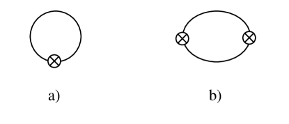
FIG. 4.1.: Two kinds of one-loop graphs generated by pseudoscalar mesons, which relate to calculation in this section. a) Tadpole diagram. b) Two-point corrector.

There are several remarks relating to our calculation, 1) Since $m_{\pi}^{2}\ll m_{{}_{K}}^{2}<m_{\rho}^{2}$, we treat pion as massless particle but $m_{{}_{K}}\neq 0$ in interal line. Moreover, since difference between $m_{\eta_{8}}$ and $m_{{}_{K}}$ is small, we set $m_{\eta_{8}}=m_{{}_{K}}$ in this section. 2) Since we focus our attention on $m_{\rho}$-energy scale, we set current quark masses are zero in the following. 3) There are only two diagrams relating to our calcuation on all potential irreducible one-loop graphs. They are tadpole diagram(figure 4.1-a) and diagram including one-loop with two external source(see figure(4.1-b), hereafter we call contribution generate by this kinds of diagrams as two-point corrector).

A Four pseudoscalar meson vertex

The four pseudoscalar meson vertex relates to our following calculation which can be obtained from Eqs.( 3.11) and ( 3.24). Recalling $m_{\pi}^{2}=0$ but $m_{\eta_{8}}^{2}=m_{{}_{K}}^{2}\neq 0$, we can see that only $K$ and $\eta_{8}$ mesons can yields non-zero contribution of tadpole diagram, since in dimensional regularization, $\int d^{D}k(k^{2}+i\epsilon)^{-1}\equiv 0$. Obviously, the tadpole diagram contributes a factor which is proportional to $m_{{}_{K}}^{2}$ and momentum-independent. Thus tadpole-loop correction generated by ${\cal L}_{2}$ is nothing other than renormalization of $f_{\pi}$. Here we calculate the tadpole-loop correction generated by ${\cal L}^{\prime}_{4P}$. The calculation on two-point corrector of four pseudoscalar meson vertex will be included in the following section so that we need not calculate it here.

It is convenient to calculate meson loops in terms of background field method. To expand pseudoscalar meson fields around their classic solution

$$U(x)=\bar{\xi}(x)e^{i\varphi}\bar{\xi}(x),\hskip 72.26999pt\bar{U}(x)=\bar{\xi}^{2}(\Phi),$$ (4.1)

where background $\bar{U}(x)$ is solution of classic motion of pseudoscalar mesons, $\delta{\cal L}/\delta U(x)=0$, $\varphi(x)$ is quantum fluctuation fields around this classic solution. Inserting Eq.( 4.1) into the effective lagrangian in sect. 3 and retain terms to quadratic form of quantum fields, the one-loop effects of pseudoscalar meson can be obtained via integrating over ths quantum fields.

Then tadpole-loop contribution to 4-pseudoscalar meson vertex can be obtained via the following intregral

$$\Pi_{\rm tad}^{(4P)}=i\int\frac{d^{4}k}{(2\pi)^{4}}\frac{i}{k^{2}-m_{{}_{K}}^{2}+i\epsilon}\frac{C(p^{2})}{4}{\cal H}^{aa},$$ (4.2)

where

$${\cal H}^{aa}[SU(3)/SU(2)]=\frac{11}{6}<\Omega_{\mu\nu}(\xi\nabla^{\mu}U^{{\dagger}}\nabla^{\nu}U\xi^{{\dagger}}+\xi^{{\dagger}}\nabla^{\mu}U\nabla^{\nu}U^{{\dagger}}\xi)>.$$ (4.3)

Substituenting Eq.( 4.3) into Eq.( 4.2), we obtain the tadpole-loop contribution to 4-pseudoscalar vertex as follow

$$\Pi_{\rm tad}^{(4P)}=-\frac{11}{24}\frac{\lambda}{(4\pi)^{2}}m_{{}_{K}}^{2}C(p^{2})<\Omega_{\mu\nu}(\xi\nabla^{\mu}U^{{\dagger}}\nabla^{\nu}U\xi^{{\dagger}}+\xi^{{\dagger}}\nabla^{\mu}U\nabla^{\nu}U^{{\dagger}}\xi)>.$$ (4.4)

where we define a parameter $\lambda$ to absorbe quadratic divergence from loop integral

$$\lambda=(\frac{4\pi\mu^{2}}{m_{{}_{K}}^{2}})^{\epsilon/2}\Gamma(1-\frac{D}{2}).$$ (4.5)

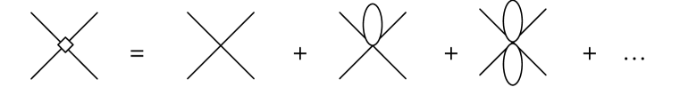
FIG. 4.2.: Four-pseudoscalar meson vertex with tadpole diagram correction. Here $``\diamond^{\prime\prime}$ denotes the vertex with correction of all tadpole diagrams.

For calculating all potential tadpole diagrams contribution, we need to sum over all diagrams in figure(4.2). Comparing Eq.( 4.4) with Eq.( 3.24), we can see every tadpole-loop in figure(4.2) contributes a factor

$$-\frac{11}{3}\zeta,\hskip 72.26999pt(\zeta=\frac{2\lambda}{(4\pi)^{2}}\frac{m_{{}_{K}}^{2}}{f_{\pi}^{2}}).$$ (4.6)

Then to sum over all diagrams in figure(4.2), we obtain

$${\cal L}^{\prime}_{4P}=\frac{1}{16}\frac{f_{\pi}^{2}C(p^{2})}{1+11\zeta/3}<\Omega_{\mu\nu}(\xi\nabla^{\mu}U^{{\dagger}}\nabla^{\nu}U\xi^{{\dagger}}+\xi^{{\dagger}}\nabla^{\mu}U\nabla^{\nu}U^{{\dagger}}\xi)>.$$ (4.7)

For the sake of convenience of calculation on two-point corrector in the following subsections, we like to divid quantum pseudoscalar fields from lagrangian ${\cal L}_{2}$ and ${\cal L}^{\prime}_{4P}$ in terms of background field method. Those quantum pseudoscalar fields contract to internal lines in figure(4.1-b).

Inserting Eq.( 4.1) in to lagrangian ${\cal L}_{2}$ and retaining terms to quadratic form of quantum fields we obtain

$${\cal L}_{2}=\bar{{\cal L}}_{2}+\frac{f_{\pi}^{2}}{16}<d_{\mu}\varphi d^{\mu}\varphi-[\Delta_{\mu},\varphi][\Delta^{\mu},\varphi]>.$$ (4.8)

Then interaction vertices including two quantum fields is

$$\delta{\cal L}_{2}=\frac{1}{4}<2\Gamma_{\mu}[\varphi,\partial^{\mu}\varphi]+[\Gamma_{\mu},\varphi][\Gamma^{\mu},\varphi]-[\Delta_{\mu},\varphi][\Delta^{\mu},\varphi]>,$$ (4.9)

where quantum field has been normalized, and only background fields are included in $\Gamma_{\mu}$ and $\Delta_{\mu}$,

$$\Gamma_{\mu}=-i\gamma_{\mu}+\Omega_{\mu}=-i\gamma_{\mu}+\frac{1}{8}[\Phi,\partial_{\mu}\Phi]+...,\hskip 72.26999pt\gamma_{\mu}=e{\cal Q}A_{\mu},$$ (4.10)

where $\Phi$ is background fields. In lagrangian( 4.9), only first term relates to our following calculation.

Inserting Eq.( 4.1) into Eq.( 4.7) and retaining terms to quadratic form of quantum fields we have

$$\delta{\cal L}^{\prime}_{4P}(p^{2})=\frac{1}{2}\frac{C(p^{2})}{1+11\zeta/3}<\Omega_{\mu\nu}[\partial^{\mu}\varphi,\partial^{\nu}\varphi]>,$$ (4.11)

where $p$ is momentum of $\Omega_{\mu}$ and independent of loop integral. This is only term which survives when coupled to conserved current or on-shell vector mesons. Eq.( 4.11) together with Eq.( 4.9) lead to all 4-pseudoscalar meson vertex which relates to our the following calculation,

$$\delta{\cal L}_{4P}=\frac{1}{2}[\delta_{\mu\nu}+\frac{C(p^{2})}{1+11\zeta/3}(p^{2}\delta_{\mu\nu}-p_{\mu}p_{\nu})]<\Omega^{\mu}[\varphi,\partial^{\nu}\varphi]>.$$ (4.12)

B Correction to $\gamma\rightarrow\pi\pi$ vertex

1 Tadpole diagram

The effective lagrangian can generate non-trivial tadpole-loop contribution, which corrects to $\gamma\rightarrow\varphi\varphi$ vertex(see figure(4.3)). Obviously, the correction of tadpole diagram is proportional to $m_{{}_{K}}^{2}$ and momentum-independent. Thus tadpole-loop correction generated by ${\cal L}_{2}$ is nothing other than renormalization of $f_{\pi}$. Here we calculate the tadpole-loop correction generated by ${\cal L}^{\prime}$. In terms of background method, we can insert Eq.( 4.1) into lagrangian ( 3.22) and retain terms to quadratic form of quantum fields. Then we obtain

$$\delta{\cal L}_{\rm tad} = \frac{i}{2}b(p^{2})<(\xi\gamma^{\mu\nu}\xi^{{\dagger}}+\xi^{{\dagger}}\gamma^{\mu\nu}\xi)(\Delta_{\mu}\varphi\Delta_{\nu}\varphi+\varphi\Delta_{\mu}\Delta_{\nu}\varphi+\varphi\Delta_{\mu}\varphi\Delta_{\nu}$$ (4.14)

$$\hskip 72.26999pt-\frac{3}{2}\Delta_{\mu}\Delta_{\nu}\{\varphi,\varphi\})>,$$

where $\varphi$ has been normailzed.

Due to completeness relation of generators of SU(N) group ( 3.8), we have

$$\Pi_{\rm tad}^{\gamma\varphi\varphi}=\frac{3i}{4}\frac{\lambda}{(8\pi)^{2}}m_{{}_{K}}^{2}gb(p^{2})<\gamma_{\mu\nu}(\nabla^{\mu}U^{{\dagger}}\nabla^{\nu}U+\nabla^{\mu}U\nabla^{\nu}U^{{\dagger}})>.$$ (4.15)

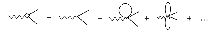
FIG. 4.3.: $\gamma\rightarrow\varphi\varphi$ vertex with correction of all tadpole diagrams.

Comparing Eq.( 4.15) with Eq.( 3.22), we can see that every tadpole-loop in figure(4.3) yields a factor $-3\zeta$. To sum over all diagrams in figure(4.3), we obtain the $\gamma\rightarrow\varphi\varphi$ vertex with tadpole diagram correction as follow

$${\cal L}^{(1)}_{\gamma\varphi\varphi}=-\frac{i}{2}<\gamma_{\mu}[\varphi,\partial^{\mu}\varphi]>-\frac{i}{4}\frac{gb(p^{2})}{1+3\zeta}<\gamma_{\mu\nu}[\partial^{\mu}\varphi,\partial^{\nu}\varphi]>,$$ (4.16)

where the quantum field $\varphi$ has been normalized.

2 Two-point corretor

  a.

$\gamma\rightarrow\varphi\varphi$ vertex generated by ${\cal L}_{2}$

In this case, the tree level $\gamma\rightarrow\varphi\varphi(\varphi=\pi,K)$ vertex reads from the first term of Eq.( 4.16), and 4-$\varphi$ vertices is given in Eq.( 4.12). The calculation is straightforward

$$G_{1}(p) = \frac{i}{4}<\gamma_{\mu}[\lambda^{a},\lambda^{b}]><\Omega^{\alpha}[\lambda^{a},\lambda^{b}]>[\delta_{\alpha\beta}+\frac{C(p^{2})}{1+11\zeta/3}(p^{2}\delta_{\alpha_{\beta}}-p_{\alpha}p_{\beta})]$$ (4.18)

$$\times\int\frac{d^{4}k}{(2\pi)^{4}}\frac{i}{k^{2}-m_{\varphi}^{2}+i\epsilon}\frac{i}{(k+p)^{2}-m_{\varphi}^{2}+i\epsilon}k^{\mu}(2k+p)^{\beta},$$

where $p$ is momentum of photon. Employing completeness relation of generators of SU(N) group ( 3.8), we obtain

$$<A[\lambda^{a},\lambda^{b}]><B[\lambda^{a},\lambda^{b}]>=-8N<AB>+8<A><B>.$$ (4.19)

Then recalling massless pion and U(1)_e.m. guage invariant, we obtain SU(2) correction of Eq.( 4.18) as follow

$$G_{1}[SU(2)] = \frac{i}{2}(p^{2}\delta_{\mu\nu}-p_{\mu}p_{\nu})<\gamma^{\mu}[\Phi,\partial^{\nu}\Phi]>\{[\frac{\lambda}{96\pi^{2}}+\frac{1}{16\pi^{2}}\int_{0}^{1}dx\cdot x(1-x)\ln{\frac{x(1-x)p^{2}}{m_{{}_{K}}^{2}}}$$ (4.22)

$$+\frac{i}{96\pi^{2}}Arg(-1)\theta(p^{2}-4m_{\pi}^{2})]-\frac{C(p^{2})}{1+11\zeta/3}\frac{p^{2}}{(4\pi)^{2}}[\frac{\lambda}{6}$$

$$+\int_{0}^{1}dx\cdot x(1-x)\ln{\frac{x(1-x)p^{2}}{m_{{}_{K}}^{2}}}+\frac{i}{6}Arg(-1)\theta(p^{2}-4m_{\pi}^{2})]\},$$

where

$$Arg(-1) = (1+2k)\pi,\hskip 72.26999ptk=0,\pm 1,\pm 2,...,$$ (4.23)

$$\theta(x-y) = \left\{{1;\hskip 57.81621ptx>y\atop 0.\hskip 57.81621ptx\leq y}\right.$$ (4.24)

We can see that one-loop of pion contributes to a large imaginary part of ${\cal T}$-matrix.

Since in this paper we pay our attention on energy scale $p^{2}<4m^{2}\simeq 4m_{{}_{K}}^{2}$, there is no imaginary part yielded by $K$-loop. Then we can obtain SU(3)/SU(2) correction of Eq.( 4.18) as follow

$$G_{1}[SU(3)/SU(2)]\hfill$$ (4.25)

$$= -\frac{i}{4}(p^{2}\delta_{\mu\nu}-p_{\mu}p_{\nu})<\gamma^{\mu}[\Phi,\partial^{\nu}\Phi]>\{[\frac{\lambda}{96\pi^{2}}-\frac{1}{16\pi^{2}}\int_{0}^{1}\cdot x(1-x)\ln{(1-\frac{x(1-x)p^{2}}{m_{{}_{K}}^{2}})}]$$ (4.27)

$$-\frac{C(p^{2})}{1+11\zeta/3}\frac{1}{(4\pi)^{2}}[\lambda(\frac{p^{2}}{6}-m_{{}_{K}}^{2})-\int_{0}^{1}dx\cdot[m_{{}_{K}}^{2}-x(1-x)p^{2}]\ln{(1-\frac{x(1-x)p^{2}}{m_{{}_{K}}^{2}})}]\}.$$

Defining

$$D(p^{2}) = \frac{1}{16\pi^{2}f_{\pi}^{2}}\{\lambda+\int_{0}^{1}dx\cdot x(1-x)\ln{[(1-\frac{x(1-x)p^{2}}{m_{{}_{K}}^{2}})(\frac{x(1-x)p^{2}}{m_{{}_{K}}^{2}})^{2}]}$$ (4.29)

$$\hskip 36.135pt+\frac{2}{3}Arg(-1)\theta(p^{2}-4m_{\pi}^{2}),$$

$$\Sigma_{0}(p^{2}) = \frac{1}{8\pi^{2}f_{\pi}^{2}}\{\lambda(\frac{p^{2}}{2}-m_{{}_{K}}^{2})-\int_{0}^{1}dx\cdot[m_{{}_{K}}^{2}-x(1-x)p^{2}]\ln{(1-\frac{x(1-x)p^{2}}{m_{{}_{K}}^{2}})}$$ (4.31)

$$+2p^{2}\int_{0}^{1}dx\cdot x(1-x)\ln{\frac{x(1-x)p^{2}}{m_{{}_{K}}^{2}}}+p^{2}\frac{i\pi}{3}Arg(-1)\theta(p^{2}-4m_{\pi}^{2})\},$$

we obtain that two-point corrector of $\gamma\rightarrow\varphi\varphi$ vertex which generated by ${\cal L}_{2}$ as follow

$$G_{1}^{\gamma\varphi\varphi} = \frac{i}{8}f_{\pi}^{2}[D(p^{2})+\frac{C(p^{2})\Sigma_{0}(p^{2})}{1+11\zeta/3}](p^{2}\delta_{\mu\nu}-p_{\mu}p_{\nu})<\gamma^{\mu}[\Phi,\partial^{\nu}\Phi]>$$ (4.32)

$$\rightarrow \frac{i}{8}f_{\pi}^{2}[D(p^{2})+\frac{C(p^{2})\Sigma_{0}(p^{2})}{1+11\zeta/3}]<\gamma_{\mu\nu}(\nabla^{\mu}U^{{\dagger}}\nabla^{\nu}U+\nabla^{\mu}U\nabla^{\nu}U^{{\dagger}})>.$$ (4.33)

This effective vertex is $O(p^{4})$ at least.

  b.

$\gamma\rightarrow\varphi\varphi$ vertex generated by high order lagrangian

Since Eq.( 4.32) and the second term of Eq.( 4.16) are same level in momentum expasion, we can calculate two-point corrector generated by them simultaneously. Combining Eqs.( 4.32) and the second term of ( 4.16), we have

$${\cal L}^{\prime}=-\frac{i}{2}b_{\gamma}(p^{2})<\gamma_{\mu\nu}[\partial^{\mu}\varphi,\partial^{\nu}\varphi]>,$$ (4.34)

where

$$b_{\gamma}(p^{2})=\frac{gb(p^{2})}{2(1+3\zeta)}-D(p^{2})-\frac{C(p^{2})\Sigma_{0}(p^{2})}{1+11\zeta/3}.$$ (4.35)

Then we obtain two-point corrector generated by ${\cal L}^{\prime}$ as follow

$$G_{2}^{\gamma\varphi\varphi}(p) = -\frac{N}{2}b_{\gamma}(p^{2})<\gamma_{\mu\nu}[\Phi,\partial^{\alpha}\Phi]>[\delta_{\alpha\beta}+\frac{C(p^{2})}{1+11\zeta/3}(p^{2}\delta_{\alpha_{\beta}}-p_{\alpha}p_{\beta})]$$ (4.37)

$$\times\int_{0}^{1}dx\int\frac{d^{4}k}{(2\pi)^{4}}\frac{p^{\mu}k^{\nu}k^{\beta}}{[k^{2}-m_{\varphi}^{2}+x(1-x)p^{2}+i\epsilon]^{2}}.$$

In case of SU(2), the above equation is rewritten as follow

$$G_{2}[SU(2)] = \frac{i}{2}b_{\gamma}(p^{2})[1+\frac{p^{2}C(p^{2})}{1+11\zeta/3}]<\gamma_{\mu\nu}[\partial^{\mu}\Phi,\partial^{\nu}\Phi]>\frac{p^{2}}{(4\pi)^{2}}$$ (4.39)

$$\times\{\frac{\lambda}{6}+\int_{0}^{1}dx\cdot x(1-x)\ln{\frac{x(1-x)p^{2}}{m_{{}_{K}}^{2}}}+\frac{i}{6}Arg(-1)\theta(p^{2}-4m_{\pi}^{2})\}.$$

For massive $K$-meson, two-point corrector in SU(3)/SU(2) sector reads

$$G_{2}[SU(3)/SU(2)] = \frac{i}{4}b_{\gamma}(p^{2})[1+\frac{p^{2}C(p^{2})}{1+11\zeta/3}]<\gamma_{\mu\nu}[\partial^{\mu}\Phi,\partial^{\nu}\Phi]>\frac{1}{(4\pi)^{2}}\{\lambda(\frac{p^{2}}{6}-m_{{}_{K}}^{2})$$ (4.41)

$$-\int_{0}^{1}dx\cdot[m_{{}_{K}}^{2}-x(1-x)p^{2}]\ln{(1-\frac{x(1-x)p^{2}}{m_{{}_{K}}^{2}})}\}.$$

Eqs.( 4.41) together with Eq.( 4.39) given one-loop correction to $\gamma\rightarrow\Phi\Phi$ vertex. Defining

$$\Sigma(p^{2})=(1+\frac{p^{2}C(p^{2})}{1+11\zeta/3})\Sigma_{0}(p^{2}),$$ (4.42)

we obtain

$$G_{2}^{\gamma\varphi\varphi}=\frac{i}{8}b_{\gamma}(p^{2})f_{\pi}^{2}\Sigma(p^{2})<\gamma_{\mu\nu}[\partial^{\mu}\Phi,\partial^{\nu}\Phi]>.$$ (4.43)

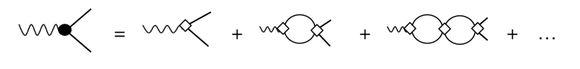
FIG. 4.4.: The chain approximation. To sum over all of those diagrams we can obtain complete $\gamma\rightarrow\pi\pi$ vertex up to one-loop level. Here $``\diamond^{\prime\prime}$ denotes every vertices have included tadpole-loop correction.

To sum over all diagrams in chain approximation(figure(4.4)), we can obtain the complete $\gamma\rightarrow\pi\pi$ vertex. Comparing Eq.( 4.43) with Eq.( 4.34), we can see that every one-loop in figure(4.4) yields a factor ($-\Sigma(p^{2})$). Thus to sum over all diagrams in figure(4.4) and together with the lowest order term, we can obtain the complete $\gamma\rightarrow\pi\pi$ vertex as follow

$${\cal L}_{\gamma\pi\pi}^{c}=-\frac{i}{2}<\gamma_{\mu}[\pi,\partial^{\mu}\pi]>-\frac{i}{2}\frac{b_{\gamma}(p^{2})}{1+\Sigma(p^{2})}<\gamma_{\mu\nu}[\partial^{\mu}\pi,\partial^{\nu}\pi]>,$$ (4.44)

where $\pi$ field has been normalized. The eq. (4.44) is important for studies on $\omega$ physics and pion form factor in elsewhere.

C Correction to $\rho\rightarrow\pi\pi$ vertex

In leading order of $N_{c}^{-1}$ expansion, the $\rho\rightarrow\varphi\varphi$ vertex read from(with physical $\rho$-field)

$${\cal L}_{\rho\varphi\varphi}=-\frac{i}{16}b(p^{2})f_{\pi}^{2}<\rho_{\mu\nu}(\xi\nabla^{\mu}U^{{\dagger}}\nabla^{\nu}U\xi^{{\dagger}}+\xi^{{\dagger}}\nabla^{\mu}U\nabla^{\nu}U^{{\dagger}}\xi)>.$$ (4.45)

Thus the calculation in this subsection is similar to one in section 4.2.2.

  a.

Tadpole diagram

In this case, $\xi$ and $\xi^{{\dagger}}$ in lagrangian ( 4.45) include quantum fields only, i.e., $\xi={\rm exp}\{i\varphi/2\}$. Then inserting Eq.( 4.1) and the above $\xi,\;\xi^{{\dagger}}$ into lagrangian ( 4.45), and retaining terms to quadratic form of quantum fields, we obtain

$$\delta{\cal L}_{\rm tad}==\frac{N}{4}ib(p^{2})\varphi^{a}\varphi^{a}<\rho_{\mu\nu}(\xi\nabla^{\mu}U^{{\dagger}}\nabla^{\nu}U\xi^{{\dagger}}+\xi^{{\dagger}}\nabla^{\mu}U\nabla^{\nu}U^{{\dagger}}\xi)>,$$ (4.46)

where quantum fields $\varphi^{a}$ have been normalized. From Eq.( 4.46), it is easily to obtain tadpole-loop contribution which is yielded by pseudoscalar mesons of SU(3)/SU(2) sector,

$$\Pi_{\rm tad}^{\rho\varphi\varphi}=\frac{i}{4}\frac{\lambda}{(4\pi)^{2}}m_{{}_{K}}^{2}b(p^{2})<\rho_{\mu\nu}(\xi\nabla^{\mu}U^{{\dagger}}\nabla^{\nu}U\xi^{{\dagger}}+\xi^{{\dagger}}\nabla^{\mu}U\nabla^{\nu}U^{{\dagger}}\xi)>.$$ (4.47)

Therefore, every tadpole-loop contributes a factor ($-2\zeta$) to $\rho\rightarrow\varphi\varphi$ vertex. To sum over all potential tadpole diagram correction, we obtain

$${\cal L}^{(1)}_{\rho\varphi\varphi}=\frac{i}{4}\frac{b(p^{2})}{1+2\zeta}<\rho_{\mu\nu}[\partial^{\mu}\varphi,\partial^{\nu}\varphi]>.$$ (4.48)

where $\varphi$ field has been normalized.

  b.

Two-point corrector

To replace $b(p^{2})/(1+2\zeta)$ in Eq.( 4.48) by $b_{\gamma}(p^{2})$ in Eq.( 4.34), we can see that the calculation on two-point corrector of $\rho\rightarrow\varphi\varphi$ vertex will be the same as one in section 4.2.2. The result can be obtained from Eq.( 4.43) directly,

$$G^{\rho\pi\pi}=\frac{i}{4}\frac{b(p^{2})}{1+2\zeta}\Sigma(p^{2})<\rho_{\mu\nu}[\partial^{\mu}\pi,\partial^{\nu}\pi]>.$$ (4.49)

To sum over all diagrams of chain approxiamtion in figure(4.4), we obtain the complete $\rho\rightarrow\pi\pi$ vertex,

$${\cal L}_{\rho\pi\pi}^{c}=-\frac{i}{4}g_{\rho\pi\pi}(p^{2})<\rho_{\mu\nu}[\partial^{\mu}\pi,\partial^{\nu}\pi]>,$$ (4.50)

where

$$g_{\rho\pi\pi}(p^{2})=\frac{b(p^{2})}{(1+2\zeta)(1+\Sigma(p^{2}))}.$$ (4.51)

D Correction to $\rho-\gamma$ vertex

The complete one-loop correction to $\rho-\gamma$ vertex contains two different ingrendients:

1) The effective lagrangian( 3.17) will generate tadpole diagram. For obtaining complete tadpole-loop correction, we need to sum over all tadpole-loop diagrams in figure(4.5).

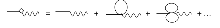
FIG. 4.5.: The $\rho-\gamma$ vertex with correction by all tadpole diagrams.

2) The chain approximation correction in figure(4.6). Here these loop graphs are generated by $\rho\rightarrow\varphi\varphi$, 4-pseudoscalar and $\gamma\rightarrow\varphi\varphi$ vertices. All vertices should include correction of all potential tadpole diagrams. These corrections have been obtained in section 4.1, 4.2 and 4.3.

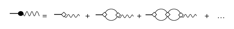
FIG. 4.6.: Chain approximation to $\rho-\gamma$ couping, which is generated by $\rho\rightarrow\varphi\varphi$, 4-pseudoscalar and $\gamma\rightarrow\varphi\varphi$ vertices. Here $``\diamond^{\prime\prime}$ denotes every vertices are with complete tadpole-loop correction.

Note that Only pseudoscalar mesons in SU(3)/SU(2) sector yield tadpole-loop contribution. Then fig.(4.5) and fig.(4.6) lead to complete $\rho-\gamma$ coupling vertex as follow

$${\cal L}_{\rho\gamma}^{c}=-\frac{b_{\rho\gamma}(p^{2})}{4}<\rho_{\mu\nu}\gamma^{\mu\nu}>,$$ (4.52)

where

$$b_{\rho\gamma}(p^{2})=\frac{A(p^{2})}{g(1+\zeta)}-f_{\pi}^{2}b(p^{2})\frac{\Sigma_{0}(p^{2})}{1+2\zeta}[1+\frac{p^{2}b_{\gamma}(p^{2})}{1+\Sigma(p^{2})}].$$ (4.53)

E Unitarity and propagator of $\rho$-meson

The unitarity must be staified for every reliable theory. In this subsection we will examine unitarity of this present formalism via forward scattering of $\rho$-meson. The examination on other processes can be performed similarly. We define $S$-matrix and ${\cal T}$-matrix as usual,

$$<\beta|S(=Te^{i\int d^{4}x{\cal L}(x)})|\alpha>=S_{\beta,\alpha}=\delta_{\beta,\alpha}+i\delta^{(4)}(p_{\beta}-p_{\alpha}){\cal T}_{\beta,\alpha}.$$ (4.54)

The unitarity requires

$${\rm Im}{\cal T}_{\beta,\alpha}=\frac{1}{2}\int d\Psi\delta^{(4)}(p_{\Psi}-p_{\alpha}){\cal T}_{\Psi,\alpha}^{*}{\cal T}_{\Psi,\beta},$$ (4.55)

where $\Psi$ is all potential physics states. For the case of $\alpha=\beta=\rho$, $<\Psi|=<\pi\pi|$ is dominant. Then for forward scattering of $\rho$-meson, Eq.( 4.45) becomes

$$\Gamma(\rho\rightarrow\pi\pi)=\frac{2}{(2\pi)^{4}}{\rm Im}{\cal T}_{\rho\rho}.$$ (4.56)

The width $\Gamma(\rho\rightarrow\pi\pi)$ can be obtained from the complete vertex( 4.50),

$$\Gamma(\rho\rightarrow\pi\pi)=\frac{|g_{\rho\pi\pi}(m_{\rho}^{2})|^{2}m_{\rho}^{5}}{48\pi}(1-\frac{4m_{\pi}^{2}}{m_{\rho}^{2}})^{3/2}.$$ (4.57)

For obtaining ${\rm Im}{\cal T}_{\rho\rho}$, we need to calculate chain-approximation correction of pseudoscalar loops for two-point vertex of $\rho$-meson. The calculation is similar to one in section 4.3. To use the equation of motion of $\rho$-meson, eq. (3.14), and renormalize the mass of $\rho$-meson, we have

$${\cal L}_{\rho\rho}^{1-{\rm loop}}=i{\rm Im}[\Sigma_{0}(m_{\rho}^{2})\frac{f_{\pi}^{2}m_{\rho}^{4}b^{2}(m_{\rho}^{2})}{g^{2}(1+2\zeta)^{2}(1+\Sigma(m_{\rho}^{2}))}]\rho_{\mu}^{i}\rho^{i\mu}.$$ (4.58)

where $\rho$-field has been normalized.

Since Im$(\Sigma_{0}\cdot\Sigma)\equiv 0$, we obtain

$$\frac{2}{(2\pi)^{4}}{\rm Im}{\cal T}_{\rho\rho}=-2[{\rm Im}\Sigma_{0}(m_{\rho}^{2})]\frac{f_{\pi}^{2}m_{\rho}^{3}g^{-2}b^{2}(m_{\rho}^{2})}{(1+2\zeta)^{2}|1+\Sigma(m_{\rho}^{2})|^{2}}.$$ (4.59)

Setting $Arg(-1)=-\pi$ in Eq.( 4.62), we have

$${\rm Im}\Sigma_{0}(m_{\rho}^{2})=-\frac{m_{\rho}^{2}}{24\pi f_{\pi}^{2}}\theta(m_{\rho}^{2}-4m_{\pi}^{2})\equiv-\frac{m_{\rho}^{2}}{24\pi f_{\pi}^{2}}.$$ (4.60)

Inserting Eq.( 4.60) into Eq.( 4.59) and comparing with Eq.( 4.57), we can see unitary condition (4.56) is satisfied at the limit of massless pion. In addition, the difference between Eqs.( 4.57) and (4.60) implies that we can perform the following replacement

$$\theta(m_{\rho}^{2}-4m_{\pi}^{2})\rightarrow(1-\frac{4m_{\pi}^{2}}{m_{\rho}^{2}})^{3/2}.$$ (4.61)

This replacement will compensate for the approximation of massless pion. In terms of similar method, we can also prove unitarity on $\rho^{0}\rightarrow\gamma\rightarrow e^{+}e^{-}$ decay.

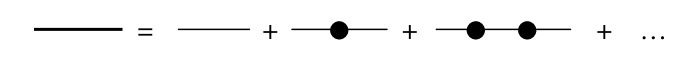
FIG. 4.7.: The complete propagator of $\rho$-meson. Here “$\bullet$” denotes the two-point vertex generated by meson-loop.

Finally, the complete propagator of $\rho$-meson can be obtained via chain approximation in figure(4.7), where every “$\bullet$” denotes a two-point vertex ( 4.58). The result is

$$\Delta_{\mu\nu}^{(\rho)}(p^{2})=\frac{-i}{p^{2}-m_{\rho}^{2}+im_{\rho}\Gamma_{\rho}}(\delta_{\mu\nu}-(\propto\frac{p_{\mu}p_{\nu}}{m_{\rho}^{2}})\;{\rm term}).$$ (4.62)

where the width $\Gamma_{\rho}\simeq\Gamma(\rho\rightarrow\pi\pi)$ which is given in Eq.( 4.57). In this paper since we treat $\rho$-meson at tree level, the $(\propto p_{\mu}p_{\nu}/m_{\rho}^{2})$ term in the propagator is unimportant. Then the propagator( 4.62) is just well-know Breit-Wigner formula for resonances.

F Cancellation of divergence

From the above calculations we can find that there is only quadratic divergence appears in one-loop contribution of pseudoscalar mesons. Since the present model is a non-renormalizable effective theory, these divergences have to be factorized, i.e., the parameter $\lambda$ has to be determined phenomenologically. Fortunately, this parameter can be fitted by Zweig rule.

The on-shell decay $\phi\rightarrow\pi\pi$ is forbidden by G parity conservation and Zweig rule. Experiment also show that branching ratios of this decay is very small, $B(\phi\rightarrow\pi\pi)=(8\;{+5\atop-4})\times 10^{-5}$. Theoretically, this decay can occur through photon-exchange or $K$-loop(figure(4.8)). The latter two diagrams yield non-zero imagnary part of decay amplitude. Thus the real part yielded by the latter two diagrams should be very small. We can determine $\lambda$ due to this requirement(the chiral expansion in powers of $\phi$-mass will be studied in other papers, but it do not affect us to fit $\lambda$ here). From the calculation in the above section, we see that the result yielded by the latter two diagrams is proportional to a factor

$$\lambda(\frac{p^{2}}{2}-m_{{}_{K}}^{2})-\int_{0}^{1}dx\cdot[m_{{}_{K}}^{2}-x(1-x)p^{2}]\ln{(1-\frac{x(1-x)p^{2}}{m_{{}_{K}}^{2}})}|_{p^{2}=m_{\phi}^{2}}.$$ (4.63)

Since we only focus our attention on real part of the above equation, $m_{\phi}^{2}=4m_{{}_{K}}^{2}$ is a enough approximation. Then Zweig rule requires that

$$\lambda(\frac{p^{2}}{2}-m_{{}_{K}}^{2})-Re\{-\int_{0}^{1}dx\cdot[m_{{}_{K}}^{2}-x(1-x)p^{2}]\ln{(1-\frac{x(1-x)p^{2}}{m_{{}_{K}}^{2}})}\}|_{p^{2}=4m_{{}_{K}}^{2}}\simeq 0.$$ (4.64)

Form the above equation, we obtain

$$\lambda\simeq\frac{2}{3}.$$ (4.65)

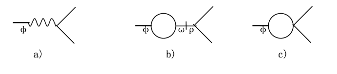
FIG. 4.8.: Some diagrams for $\phi\rightarrow\pi\pi$ decay. The one-loop in figure b) and c) is $K$-loop.

V Numerical Results and Discussion

In this section we will calculate on-shell $\rho\rightarrow\pi\pi$ and $\rho^{0}\rightarrow e^{+}e^{-}$ decay numerically. The following parameters will relate to our calculation: The constituent quark mass $m\simeq 480$MeV is fitted by chiral coupling constants of ChPT at $p^{4}$. The universal coupling constant $g=\pi^{-1}$ is determined by KSRF(I) sum rule and $\lambda\simeq\frac{2}{3}$ is determined by Zweig rule. Other parameters $f_{\pi}=185$MeV, $m_{\rho}=770$MeV and $m_{{}_{K}}=495$MeV are fitted by experimental data. The formula for $\rho\rightarrow\pi\pi$ decay width has been given in Eq.( 4.57), and the width of $\rho^{0}\rightarrow e^{+}e^{-}$ decay is given as follow

$$\Gamma(\rho^{0}\rightarrow e^{+}e^{-})=\frac{4\pi}{3m_{\rho}^{3}}|g_{\rho\gamma}(m_{\rho}^{2})|^{2}\alpha^{2},$$ (5.1)

with

$$g_{\rho\gamma}(p^{2})=\frac{b_{\rho\gamma}(p^{2})}{2g}p^{2},$$ (5.2)

where $b_{\rho\gamma}$ was given in Eq.( 4.53). Then we obtain $\Gamma(\rho\rightarrow\pi\pi)$=146MeV and $\Gamma(\rho^{0}\rightarrow e^{+}e^{-})$=7.0MeV. These value agree with data excellently.

	I)	II)	III)	Expertiment
$\Gamma(\rho\rightarrow\pi\pi)$(MeV)	125	182	146	150
$\Gamma(\rho^{0}\rightarrow e^{+}e^{-})$(KeV)	4.32	7.76	7.0	$6.77\pm 0.32$
$|f_{\rho\pi\pi}(m_{\rho}^{2})|$	5.51	6.62	5.94	-
$|g_{\rho\gamma}(m_{\rho}^{2})|$(GeV2)	0.094	0.126	0.12	-
$\frac{1}{2}|f_{\rho\pi\pi}(m_{\rho}^{2})|f_{\pi}^{2}$(GeV2)	0.094	$0.114^{a)}$	$0.1^{a)}$	-

TABLE II.: The widths of $\rho\rightarrow\pi\pi$ and $\rho\rightarrow e^{+}e^{-}$ decays. I) The values at leading order of momentum expansion and without meson-loop correction. II) The values with all order of momentum expansion but without meson-loop correction. III) The values with all order momentum expansion and with meson-loop correction. a) Comparing $\frac{1}{2}f_{\rho\pi\pi}(m_{\rho}^{2})f_{\pi}^{2}$ with $g_{\rho\gamma}(m_{\rho}^{2})$, we can obtain the broken of KSRF(I) sum rule.

In table 2 we compare the widths of $\rho\rightarrow\pi\pi$ and $\rho\rightarrow e^{+}e^{-}$ decays for three different cases. It clearly shows that, both of the high order terms of the momentum expansion and pseudoscalar meson-loop play very important role in chiral expansion at $m_{\rho}$-scale. The reason is obvious, that at this energy scale, the momentum expansion converge slowly, and it is not enough to merely consider the leading order terms of $N_{c}^{-1}$ expansion(or meson-loop expansion). Thus in a reliable and consistent field theory describing physics at vector meson energy scale, the leading order theoretical prediction must not agree with experimental data. Otherwise the important high order correction will become incomprehensible in logic and phenomenology. For example, from table 2 we can see that the correction of meson-loop is about $20\%$. It is agree with $N_{c}^{-1}$ expansion for $N_{c}=3$ very well. In particular, we can not understand the unitarity of this model at all if our studies are limited to capture merely the leading order effects of large $N_{c}$ expansion.

In table 2 we also show how KSRF(I) sum rule is broken. We can see that both of high power terms of momentum expansion and meson-loop break KSRF(I) sum rule. This mechanism is agree with experiment very well.

VI Summary

The physics on vector meson resonances has been studied continually by various chiral models during the last two decades. It is well known, however, that all past studies on this sort of chrial models suffer two difficulties: 1) The convergence of the chiral expansiom in the models is unclear. 2) There is no well-defined way to calculate the next to leading order. This makes the model’s calculations being not controlled approximations in that there is no well-defined way to put error bars on the predictions. In this present paper, we have provided a self-consistent pattern to overcome the difficuties mentioned above, that is the ChCQM formalism. The chiral constituent quark model with vector meson fields is formulated only by two basic ideas: One is transformation properties of relevant fields under SU(3)${}_{{}_{V}}$ and another one is to treat vector mesons as composited fields of constituent quarks. Employing ChCQM, we have provided a systematical method to investigate the chiral expansion up to all order, and to perform the calculation to the next leading order of $N_{c}^{-1}$ expansion. The results are factorized in $f_{\pi}$, $m_{0}(m_{\rho})$, $B_{0}$, $g_{A}(=0.75$, $\beta$ decay of neutron), $g(=\pi^{-1}$, KSRF(I) sum rule), $m(=480$MeV, chiral coupling constants at $p^{4}$) and $\lambda(=2/3$, Zweig rule). There are no adjustable parameters in the theoretical calculations presented in this formalism. By using this method, $\rho\rightarrow\pi\pi$ and $\rho\rightarrow e^{+}e^{-}$ decays are calculated. The predictions are in quite well agreement with the data.

Consequently, we conclude that, in ChCQM formalism we can derive a self-consistent effective field theory with the lowest vector meson resonances, and the calculation pattern presented in this paper is legitimat.

The investigation of this paper reveals the following important features of effective field theory with the lowest vector meson resonances:

i) The chiral expansion at this energy scale is convergent. The convergence of chiral expansion is the most important criterion to examine whether a chiral model including meson resonances can construct a consistent effective field theory. From this point, many approachs can only be thought of phenomenological models available at the leading order of the chiral expansion, since in those models it is diffcult to yield convergent chiral expansion at vector mesom energy scale.

ii) The chiral expansion at this energy scale converge slowly. Theoretically, it has been shown by agurement in ChPT, that the chiral expansion at energy scale $\mu$ should be in powers of $\mu^{2}/\Lambda^{2}_{\rm CSSB}$. Therefore, at $\mu\sim m_{\rho}$, complete theoretical predictions have to include high order terms of the chiral expansion, and the method of ChPT becomes impratical. Thus in this paper, we studied the chiral expansion in powers of $m_{\rho}$ systematically by means of the approach of the chiral constituent quark model. The advantage of this approach is that we can study the chiral expansion up to all orders but without extra free parameters. Although the number of parameters is even less than $O(p^{4})$ ChPT, this theory’s prediction potential is quite powerful.

iii) The large $N_{c}$ expansion argues that both of width of meson resonances and loop effects of mesons are suppressed[20]. For example, in those processes relating to $\rho$-resonance, the contribution from meson loops is about $\Gamma_{\rho}/m_{\rho}\sim 20\%$. This arguement is comfirmed by unitarity of the chiral theory(e.g., see Eq.( 4.56)). Thus the loop effects of mesons also play important role in a chiral effective theory. In this paper, we study one-loop effects of pseudoscalar mesons systematically. The logarithmic divergence and quadratic divergence from meson loops are cancelled by $O(p^{4})$ coupling constants of ChPT and Zweig rule respectively. The contribution from meson loops is about $20\%-30\%$, which agree with large $N_{c}$ arguement very well. More important, unitarity of this chiral effective theory is examined explicitly, and the one-loop correction of pseudoscalar mesons make theoretical predition close to experiment. It shows that calculation on one-loop graphs of mesons is self-consistent. All of these imply that precise prediction of a chiral meson effective theory must include the contribution from meson loops.

iv) The low energy limit of this model agree with ChPT very well. It means that at very low energy, this effective model will return to ChPT.

v) Those phenomenological successful ideas, such as VMD and universal coupling for vector meson resonances, can be predicted by this effective theory. It is quite nature in the formalism of ChCQM.

Finally, the calculation on $\rho$-meson in this paper can be easily extend to cases including $K^{*}(892)$ and $\phi(1020)$. The difference is that the strange quark mass play important role in the chiral expansion at $m_{{}_{K^{*}}}$ or $m_{\phi}$-scale. These studies will be found elsewhere.

ACKNOWLEDGMENTS

We would like to thank Prof. D.N. Gao and Dr. J.J. Zhu for their helpful discussion. This work is partially supported by NSF of China through C. N. Yang and the Grant LWTZ-1298 of Chinese Academy of Science.

REFERENCES

- [1] J.Gasser and H.Leutwyler,Ann. Phys. 158(1984) 142; Nucl. Phys. B250(1985) 465.
- [2] M. Bando, T. Kugo and K. Yamawaki, Nucl. Phys. B259 (1985) 493; ibid., Prog. Theor. Phys. 79 (1988) 1140;ibid., Phys. Rep. 164 (1988) 217; N. Kaiser and U.G. Meissner, Nucl. Phys. A519 (1990) 671.
- [3] G.Ecker, J.Gasser, A.Pich and E.de Rafel, Nucl.Phys., B321(1989) 311; G.Ecker, H.Leutwyer, J.Gasser, A.Pich and E.de Rafel, Phys.Lett.223(1989) 425.
- [4] M. Brise, Z. Phys., 355 (1996) 231.
- [5] J. Bijnens, P. Gosdzinsky and P. Talavera, Nucl.Phys. B501 (1997) 495.
- [6] S.Weinberg, Physica A96 (1979) 327.
- [7] A. Manohar and H. Georgi, Nucl.Phys. B234 (1984) 189; H. Georgi, Weak Interactions and Modern Particle Theory (Benjamin/Cimmings, Menlo Park, CA, 1984) sect. 6.
- [8] Y.Nambu and G.Jona-Lasinio, Phys. Rev. 122 (1961) 345.
- [9] J. Bijnens, Phys. Rep. 265 (1996) 369.
- [10] T. Hatsuda and T. Kunihiro, Phys. Rep. 247 (1994) 221.
- [11] L.H.Chan, Phys. Rev. Lett. 55 (1985) 21.
- [12] B.A.Li, Phys.Rev.D52 (1995) 5165.
- [13] X.J. Wang and M.L. Yan, Jour. Phys. G24(1998) 1077.
- [14] X.-J. Wang and M.-L. Yan, hep-ph/9907321.
- [15] S. Weinberg, Phys. Rev. 166(1968) 1568.
- [16] S. Coleman, J. Wess and B. Zumino, Phys. Rev. 177(1969) 2239;C.G. Callan, S. Coleman, J. Wess and B. Zumino, ibid. 2247.
- [17] U.-G. Merissner, Phys. Rep., 161(1988) 213.
- [18] J.J.Sakurai, Currents and mesons, University of Chicago press, Chicago,(1969).
- [19] V. de Alfaro, S. Fubini, G. Furlan and C. Rossetti, Currents in hadron physics, North Holland, Amsterdam, (1973).
- [20] G. ’t Hooft, Nucl. Phys. B75 (1974) 461.
- [21] D.Espriu, E.de Rafael and J.Taron, Nucl. Phys. B345 (1990) 22.
- [22] I.Aitchson and C.M.Fraser, Phys. Rev. D31 (1985) 2605.
- [23] B.A. Li and M.L. Yan, Phys. Lett. B282 (1992) 435.
- [24] R.D. Ball, Phys. Rep. 182 (1989) 1.
- [25] J. Schwenger, Phys. Rev. 93 (1954) 615.
- [26] K. Kawarabayasi and M. Suzuki, Phys. Rev. Lett. 16 (1966) 255; Riazuddin and Fayyazuddin, Phys. Rev. 147 (1966) 1507.
- [27] M. Benayoun, S. Eidelman, K. Maltman, H.B. O’Connell, B Shwartz and A.G. Williams, Europ. Phys. J.,C2(1998) 269.