LYCEN 99132

DFTT 65/99

Of DIPS, STRUCTURES and EIKONALIZATION

P. Desgrolard(), M. Giffon(), E. Martynov(), E. Predazzi().

^1,2)Institut de Physique Nucléaire de Lyon, IN2P3-CNRS et Université
Claude Bernard,
43 boulevard du 11 novembre 1918, F-69622 Villeurbanne Cedex, France

(³)Bogoliubov Institute for Theoretical Physics, National Academy of Sciences of Ukraine, 03143, Kiev-143, Metrologicheskaja 14b, Ukraine

(⁴)Dipartimento di Fisica Teorica - Università di Torino and Sezione INFN di Torino, Italy

Abstract

We have investigated several models of Pomeron and Odderon contributions to high energy elastic $pp$ and $\bar{p}p$ scattering. The questions we address concern their role in this field, the behavior of the scattering amplitude (or of the total cross-section) at high energy, and how to fit all high energy elastic data. The data are extremely well reproduced by our approach at all momenta and for sufficiently high energies. The relative virtues of Born amplitudes and of different kinds of eikonalizations are considered. An important point in this respect is that secondary structures are predicted in the differential cross-sections at increasing energies and these phenomena appear quite directly related to the procedure of eikonalizing the various Born amplitudes. We conclude that these secondary structures arise naturally within the eikonalized procedure (although their precise localization turns out to be model dependent). The fitting procedure naturally predicts the appearance of a zero at small $|t|$ in the real part of the even amplitude as anticipated by general theorems. We would like to stress, once again, how important it would be to have at LHC both $pp$ and $p\bar{p}$ options for many questions connected to the general properties of high energy hadronic physics and for a check of our predictions.

1 Introduction

Few years ago [1], combining several of the currently used philosophies, a high quality description of existing high energy elastic $pp$ and $\bar{p}p$ scattering data was obtained. The main lessons of this study performed at the Born level were:

(1) an Odderon contribution is absolutely necessary to reproduce quantitatively well the data; while its presence is not explicitly needed at $t=0$, its inclusion is necessary to have a good fit of the other $|t|$ data, specially in the dip region and in the high-$|t|$ domain

(2) hints are found that secondary structures (diffraction-like) develop in angular distributions with increasing energies at intermediate $|t|$ values in both $pp$ and $p\bar{p}$ angular distributions.

In particular, it was suggested that such structure effects should be well visible at LHC while only extremely precise data could perhaps show the effect at RHIC energies.

However, answers to some important points are still incomplete. In particular, what is a good model for the Pomeron ? What is the behavior of the scattering amplitude at high (”asymptotic”) energy ? Are large-$|t|$ data dominated by the Odderon ? Better, does a special criterium exist proving the Odderon presence ? Can one settle the question about the sign of $\alpha_{O}(0)-1\equiv\delta_{O}$ concerning the intercept of the Odderon ? Are secondary structures always predicted at large-$|t|$ when $s$ increases, i.e. do they arise ”naturally” and are they model dependent ? What is the rôle of eikonalization ? Does an amplitude that fits well the data exhibit automatically a zero in the real part of the even component of the amplitude as required by general theorems [6]?

Only partial answers presently exist (see [7] and references therein).

The Pomeron remains a most mysterious entity in spite of its resurgence from Diffractive Deep Inelastic Scattering (DDIS) data. Many models, however, exist and we are going to probe a few. Even at low-$|t|$ (first diffraction cone), it has been shown [10] that existing data do not allow to select among Pomeron models. The present data are, very likely, not yet asymptotic; this (see [11] and references therein) makes it very difficult with the existing data to establish a definite asymptotic behavior for the amplitude.

The rôle of eikonalization has not been fully clarified in spite of having been investigated by many authors [12] but many results have been obtained recently [13, 4].

The Odderon is instrumental in reproducing the large-$|t|$ data. While $t=0$ data are presumably dominated by the Pomeron, which in this region hides the Odderon, very precise data could be useful to shed light on its existence [14].

Predictions of secondary structures have appeared many times in the past [15]. The large spectrum of predictions in the position of these secondary dips shows that things are actually more complicated than anticipated long ago [16]. It is not enough that a given scheme inherently generates oscillations (like the Bessel function of an impact parameter representation); interference effects are very important in determining their position. The model dependence of these predictions, however, is not so important; it is the prediction itself of the existence of secondary structures which matters.

In this paper, four of the above points are taken into special considerations. The first is the investigation of the rôle and properties of the different varieties of eikonalization procedures one can devise. The second concerns the appearance of secondary dips and structures. These two points are strictly interconnected, being the second, to some extent, the physical counterpart of the other. The third is devoted to the behavior of the real part of the even amplitude close to zero. The fourth concerns the rôle of the Odderon in the construction of the amplitude and in the reproduction of the data.

The eikonalization procedure and its consequences is one of the principal subjects we discuss in this paper. We briefly revise (in Sec. 3) the Ordinary Eikonalization (OE) and, after (re)discovering its limits, we proceed to discuss a one-parameter generalization called Quasi Eikonalization (QE) [12] and to propose a three-parameter extension which we term Generalized Eikonalization (GE) (see [4]). Although a useful tool to alleviate the violations of $s$-channel unitarity at some level (as emphasized in [13]), eikonalization does not mean unitarization.

The effects of Ordinary Eikonalization as compared to the use of the Born amplitude have been studied within a pure Pomeron model (without aiming at quantitatively reproducing the data), and also in a ”more realistic” model including Pomeron, Odderon and secondary Reggeons, fitted to the high energy data for $pp$ and $\bar{p}p$ elastic scattering [17]. The somewhat surprising results of this ”realistic” approach were:

(i) a failure to find within the eikonalized model as high quality a fit as within its Born approximation [18], even when readjusting the parameters and even when confining oneself to the ISR data, limited to low-$|t|$ ;

(ii) a rapid numerical convergence of the rescattering series: a limited number of rescatterings (4, in addition to the Born term) is sufficient to obtain a very good approximation at present energies ;

(iii) when rescattering corrections were taken into account, a second break in the slope revealed around $|t|\sim$ 4 GeV² in the angular distribution at 300-500 GeV, creating the seed of a diffraction-type pattern at higher energies ; this break becomes a shoulder and then a true dip moving down to $|t|\sim$ 3 GeV² when $\sqrt{s}$ increases up to 14 TeV. This substructure should be seen at LHC but might even be detected at RHIC [19] if the data are very precise.

Going one step further, the one-parameter extension (QE) and much more, the three-parameters generalization (GE) prove very useful to improve the agreement with the data and, therefore, in removing the conflict found in (i) above. In addition, it helps in understanding the appearance of secondary structures, which stirred considerable interest and which is intriguing enough that we should reconsider further both their origin and their model dependence. The variety of descriptions giving rise to these diffraction-like multiple structures may suggest them to be essentially model independent; on the other hand, this is not established in an unambiguous way and deserves further theoretical analysis. In the light of this, we have undertaken a most careful analysis of several models both eikonalized and in the Born approximation, trying to ascertain whether or not the predictions of secondary structures could be related to some general pattern. By-products of our investigation turn out to be the verification that the Odderon intercept $\alpha_{O}(0)-1\equiv\delta_{O}$ obtained in the various fits is invariably non-positive and, empirically, very close to zero and that the real part of the even amplitude has the zero predicted by general theorems [6] near $|t|=0$.

In Sec. 2, we report about several non-eikonalized models with some details on their specific Pomeron and Odderon components. In Sec. 3, we do the same about OE, QE and GE. The results are presented in Sec. 4, some general conclusions are given in Sec. 5.

2 The input Born

We focus on the (dimensionless) crossing-even and -odd amplitudes $a_{\pm}(s,t)$ of the $pp$ and $\bar{p}p$ reactions

$$a_{pp}^{\bar{p}p}(s,t)=a_{+}(s,t)\ \pm a_{-}(s,t)\ ,$$ (1)

for which we have data on :

i) total cross-sections

$$\sigma_{t}={4\pi\over s}\Im{\rm m}A(s,t=0)\ ,$$ (2)

ii) differential cross-sections

$${d\sigma\over dt}={\pi\over s^{2}}\big{|}A(s,t)\big{|}^{2}\ ,$$ (3)

iii) ratio of the real to the imaginary forward amplitudes

$$\rho={\Re{\rm e}A(s,t=0)\over\Im{\rm m}A(s,t=0)}\ .$$ (4)

The crossing even part in the Born amplitude is a Pomeron (to which a $f-$Reggeon is added) while the crossing odd part is an Odderon (plus an $\omega-$Reggeon)

$$a_{+}(s,t)=\ a_{P}(s,t)+\ a_{f}(s,t)\ ,\quad a_{-}(s,t)=\ a_{O}(s,t)+\ a_{\omega}(s,t)\ .$$ (5)

For simplicity the two Reggeons have been taken in the standard form

$$a_{R}(s,t)=a_{R}\tilde{s}^{\alpha_{R}(t)}\ e^{b_{R}t},\quad\alpha_{R}(t)=\alpha_{R}(0)+\alpha^{\prime}_{R}t\ ,\quad(R=f\,{\rm and}\,\omega)\ ,$$ (6)

where $a_{f}$ ($a_{\omega}$) is real (imaginary). We begin with trajectories whose parameters are fixed as in previous works (for example [1]) $\alpha_{f}(t)=0.69+0.84\,t$, and $\alpha_{\omega}(t)=0.47+0.93\,t$ (with $t$ in GeV²), close to the values obtained in other recent fits (e.g.  [20]). As it turns out, however, a best fit requires some variation of these parameters. Thus, at the price of economy in the parameters, we end up letting them vary.

We have investigated wide classes of choices where the input amplitude (”Born term”) for the Pomeron $a_{P}(s,t)$ and for the Odderon $a_{O}(s,t)$ is either a monopole (i.e. a simple pole in the angular momentum $J-$plane) or a ”dipole” (i.e. a linear combination of a simple pole with a double pole).

The forms of $a_{P}(s,t)$ in the case of a monopole $(M)$ and of a dipole ($D$) are

$$a_{P}^{(M)}(s,t)=a_{P}\ \tilde{s}^{\alpha_{P}(t)}e^{b_{P}t}\ ,$$ (7)

and

$$a_{P}^{(D)}(s,t)=a_{P}\ \tilde{s}^{\alpha_{P}(t)}\left[e^{b_{P}(\alpha_{P}(t)-1)}(b_{P}+\ell n{\tilde{s}})\ +\ d_{P}\ell n{\tilde{s}}\right]\ ,$$ (8)

where $a_{P}$ is real.

The difference between a monopole and a dipole results in an amplitude for the second that grows with an additional power of $\ell ns$.

The Odderon may be constructed with the same requirements. It is, however, known that the rôle of the Odderon at $t=0$ is negligible but no theoretical prescription is known as how to cut it. A simple way out is to multiply the monopole or dipole form by a convenient damping factor. We choose

$$a_{O}(s,t)=(1-\exp{\gamma t})a_{O}^{(M)}(s,t)\ ,$$ (9)

or

$$a_{O}(s,t)=(1-\exp{\gamma t})a_{O}^{(D)}(s,t)\ .$$ (10)

In (9) (or (10)), the amplitude on the r.h.s. is constructed along the same lines as in (7) (or (8)) for $a_{P}^{(M,D)}(s,t)$. $a_{P}$, however, is real while $a_{O}$ is imaginary. As usual,

$$\tilde{s}\ =\ {s\over s_{0}}\ e^{-i{\pi\over 2}}\ ,\quad(s_{0}=1\ {\rm GeV}^{2})\ ,$$ (11)

enforces $s-u$ crossing and $\alpha_{i}(t)$ are the trajectories taken, for simplicity, of the linear form

$$\alpha_{i}(t)=1+\delta_{i}+\alpha_{i}^{\prime}t\ ,(i=P,O)\ .$$ (12)

It appears impossible to discriminate between (D) or (M), on general grounds; only the phenomenological results seem to prefer (D) over (M). For the sake of economy we confine our presentation to the dipole case, which gives somewhat better phenomenological results.

Some authors maintain that a perturbative (a large-$|t|$) term behaving like $|t|^{-4}$ (and complying with perturbative QCD requirements according to [21] ) is to be added to the Odderon. When the Born amplitude is eikonalized, however, all rescattering corrections implied by eikonalization are, in principle, already taken into account. Adding another large-$|t|$ term at the Born level would mimic further rescattering corrections and would lead to double counting in the eikonalized models. We shall not consider this option.

We remark that most good fits require $\delta_{P}>0$ implying what is known as a supercritical Born Pomeron i.e. a Born amplitude which, taken at face value, will eventually exceed the Froissart-Martin [22] unitarity bound even though at extremely high energies (other kinds of troubles would arise much earlier [23]). This special violation of unitarity is removed by all kinds of eikonalization. Nevertheless, one must verify that the unitarity constraints

$$\delta_{P}\geq\delta_{O}\ ,\quad{\rm and}\quad\alpha^{\prime}_{P}\geq\alpha^{\prime}_{O}\ \ .$$ (13)

are satisfied (see [13, 24]). The slope parameter for the Pomeron, finally, is expected to be in the vicinity of its ”world” value $\alpha^{\prime}_{P}\simeq 0.25$ GeV^-2 and this turns out to be, indeed, the result of the fit (see Section 4.2).

As the last comment, we recall that, in the context of the choice of the eikonalization procedure, a singular solution is, in principle, possible, whereby the Odderon dominates over the Pomeron [13]. For the sake of completeness, we have also tried this option, unphysical as this appears but, as expected, such possibility is ruled out by the results of the fits; the fit with an Odderon dominating over the Pomeron is rather poor and unacceptable.

3 Eikonalization procedures

In eikonal models, the scattering amplitudes are expressed in the impact parameter (”$b$”) representation. First, one defines the Fourier-Bessel’s (F-B) transform of the Born amplitude

$$h^{\bar{p}p}_{pp}(s,b)={1\over 2s}\int_{0}^{\infty}a^{\bar{p}p}_{pp}(s,-q^{2})J_{0}(bq)q\,dq\quad{\rm with}\quad q=\sqrt{-t}\ .$$ (14)

This is related to the eikonal function (”eikonal” for brevity) by

$$\chi^{\bar{p}p}_{pp}(s,b)\ =\ 2\ h^{\bar{p}p}_{pp}(s,b)\ .$$ (15)

The (complete) analytical forms of the Born amplitudes (both (M) and (D)) in $b$-space are given in Appendix A.

In all eikonalization procedures, one first derives the eikonalized amplitude $H^{\bar{p}p}_{pp}(s,b)$ in the $b$-representation; the inverse F-B transform leads then to the usual eikonalized amplitude in the $s-t$ space

$$A^{\bar{p}p}_{pp}(s,t)=2s\ \int_{0}^{\infty}H^{\bar{p}p}_{pp}(s,b)J_{0}(b\sqrt{-t})b\,db\ .$$ (16)

The main technical problem of eikonalization is the derivation of $H^{\bar{p}p}_{pp}(s,b)$ once $h^{\bar{p}p}_{pp}(s,b)$ are given. In what follows we make explicit this step in, we believe, the most general form so far derived.

3.1 Ordinary and Quasi Eikonalization

In the ordinary eikonal (OE) formalism, $H^{\bar{p}p}_{pp}(s,b)$ is the sum over all rescattering diagrams in the approximation when there are only two nucleons on the mass shell in any intermediate state

$$H^{\bar{p}p}_{pp,QE}(s,b)\ =\ {1\over 2i}\left(\sum\limits_{n=1}^{\infty}{\big{[}2ih^{\bar{p}p}_{pp}(s,b)\big{]}^{n}\over n!}\right)\ .$$ (17)

This limitation neglects the possibility to take into account multiparticle states. In the quasi eikonal (QE) procedure [12], the effect of these multiparticle states in the various exchange diagrams is realized introducing one additional ”weight” parameter $\lambda$ and the eikonalized amplitude in the $b$-representation (17) is replaced by

$$H^{\bar{p}p}_{pp,QE}(s,b)\ =\ {1\over 2i}\sum\limits_{n=1}^{\infty}\lambda^{n-1}{\big{[}2ih^{\bar{p}p}_{pp}(s,b)\big{]}^{n}\over n!}\ .$$ (18)

The above series is meant to represent the sum of all possible multiple exchanges of Pomerons, Odderons and secondary Reggeons ($n=1$ corresponds to the Born approximation, $n=2$ to double exchanges, etc… ). Its explicit analytical form is

$$H^{\bar{p}p}_{pp,QE}(s,b)\ =\ {1\over 2i\lambda}\left(\exp\big{[}i\lambda\chi^{\bar{p}p}_{pp}(s,b)\ \big{]}-1\right)\ .$$ (19)

As it is obvious, the value $\lambda=1$ corresponds to OE, which appears, therefore, as a particular case of QE.

However, it is not clear why all intermediate states between the exchanges of two Pomerons or two Odderons (or between one Pomeron and one Odderon) could be described by just one and the same parameter $\lambda$ or, differently stated that all the weights for the various intermediate internal couplings (two Pomerons, two Odderons or one Pomeron and one Odderon) should be the same. It would appear more ”natural” that the various exchanges should require different weights. Differently rephrased, in the QE procedure, we do not distinguish intermediate states between $P-P,\,O-O$ and $P-O$ exchanges. Giving up this assumption gives rise to a new kind of generalized eikonal (GE) procedure where all these intermediate states may have different weights.

3.2 Generalized Eikonalization

3.2.1 with 3 $\lambda:\ \lambda_{\pm},\ \lambda_{0}.$

Consider again the separate form of the amplitude (1), and let the crossing-even and crossing-odd input in the $b$-representation be

$$h_{\pm}\equiv h_{\pm}(s,b)=\ {1\over 2s}\int_{0}^{\infty}\ dq\ q\,J_{0}(bq)\,a_{\pm}(s,-q^{2})\ ,\quad(q^{2}=-t)\ .$$ (20)

Here, postponing for a moment the consideration of the most general scheme (5) when secondary Reggeons are included, we temporarily simplify the notation for the crossing even- and the crossing odd-part as if they were made by just the Pomeron and the Odderon respectively (later, we will reinstate the complete contribution)

$$a_{+}(s,t)=\ a_{P}(s,t),\quad a_{-}(s,t)=\ a_{O}(s,t)\ .$$ (21)

A priori, we have three different configurations of exchanges in the intermediate states which we show diagrammatically in Fig. 1 and where the various possibilities, $P-P,\,O-O$ and $P-O$ are described, phenomenologically, by three constants $\lambda_{+},\,\lambda_{-},\ \lambda_{0}$.

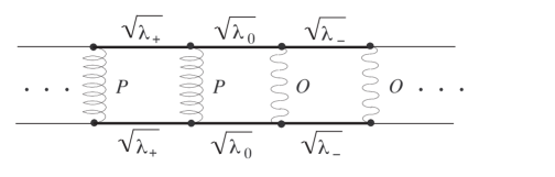
Figure 1: An example of a rescattering diagram containing the possible intermediate states with Pomeron and Odderon exchanges.

With this notation, we can deduce

$$H^{\bar{p}p}(s,b)\ =\ h_{+}\ +\ h_{-}\ +\ H[PP]+H[OO]+\ H[PO]\ +H[OP]\ .$$ (22)

where (see [4] for the details of the derivation)

$$\begin{array}[]{rll}2i\lambda_{+}H[PP]&=\sum\limits_{n=2}^{\infty}\sum\limits_{m=1}^{n-1}\sum\limits_{i=1}^{m}{1\over(m+n)!}{n-1\choose i}{m-1\choose i-1}z^{i}x^{n}y^{m}\\ \displaystyle\hfil&+\sum\limits_{n=2}^{\infty}\sum\limits_{m=n}^{\infty}\sum\limits_{i=1}^{n-1}{1\over(m+n)!}{n-1\choose i}{m-1\choose i-1}z^{i}x^{n}y^{m}+\sum\limits_{n=2}^{\infty}{1\over n!}x^{n}\\ &=z\ \sum\limits_{n=2}^{\infty}\sum\limits_{m=1}^{\infty}{x^{n}y^{m}\over(n+m)!}\ (n-1)\ _{2}F_{1}(1-m,2-n;2;z)\\ &+e^{x}-x-1\ ,\end{array}$$ (23)

$$\begin{array}[]{rll}2i\lambda_{0}H[PO]&=\sum\limits_{n=1}^{\infty}\sum\limits_{m=1}^{n}\sum\limits_{i=1}^{m}{1\over(m+n)!}{n-1\choose i-1}{m-1\choose i-1}z^{i}x^{n}y^{m}\\ &+\sum\limits_{n=1}^{\infty}\sum\limits_{m=n+1}^{\infty}\sum\limits_{i=1}^{n}{1\over(m+n)!}{n-1\choose i-1}{m-1\choose i-1}z^{i}x^{n}y^{m}\\ &=z\ \sum\limits_{n=1}^{\infty}\sum\limits_{m=1}^{\infty}{x^{n}y^{m}\over(n+m)!}\ _{2}F_{1}(1-m,1-n;1;z)\end{array}$$ (24)

with

$$x=2i\lambda_{+}h_{+}\ ,\quad y=2i\lambda_{-}h_{-}\,\quad z={\lambda_{0}^{2}\over\lambda_{+}\lambda_{-}}.$$

$H[OO]$ is obtained from $H[PP]$ with the replacement $h_{+}\longleftrightarrow h_{-}$ and $\lambda_{+}\longleftrightarrow\lambda_{-}$, and $H[OP]=H[PO]$.

The amplitude $H_{pp}(s,b)$ has the same form as $H^{\bar{p}p}(s,b)$ with the replacement $h_{-}\longleftrightarrow-h_{-}$.

Unexpectedly, one can obtain a compact analytical form from (22). Omitting all details of calculations, which can be found in [4], the final expression for the three-parameters eikonalized amplitudes are

$$\begin{array}[]{rll}H^{\bar{p}p}_{pp,GE}(s,b)&=\displaystyle{{i\over 2(\lambda_{0}^{2}-\lambda_{+}\lambda_{-})}}\bigg{\{}a+e^{\displaystyle i(\lambda_{+}h_{+}\pm\lambda_{-}h_{-})}\\ &\times\displaystyle\big{[}-a\cos{\phi_{\pm}}+i{c_{+}h_{+}\pm c_{-}h_{-}\over\phi_{\pm}}\sin{\phi_{\pm}}\big{]}\bigg{\}}\ ,\end{array}$$ (25)

where we have introduced three constants $a$ and $c_{\pm}$ defined as

$$a=2\lambda_{0}-\lambda_{+}-\lambda_{-}\ ,$$ (26)

$$c_{\pm}=\lambda_{+}\lambda_{-}-2\lambda_{0}^{2}-\lambda_{\pm}^{2}+2\lambda_{0}\lambda_{\pm}\ ,$$ (27)

in terms of the parameters of the model and the functions (of $s$ and $b$)

$$\phi_{\pm}=\sqrt{(\lambda_{+}h_{+}\mp\lambda_{-}h_{-})^{2}\ \pm 4\lambda_{0}^{2}h_{+}h_{-}}\ .$$ (28)

Considering a general case, when there are no any special relations between $\lambda_{i}$, we have found in [4] that the unitarity inequality

$$|H^{\bar{p}p}_{pp,GE}(s,b)|\leq 1$$

can be satisfied, in general, only if $\delta_{O}\leq 0$ . Two special cases, namely, $\lambda_{0}^{2}=\lambda_{-}\lambda_{+}$ (see below) and $\lambda_{+}=\lambda_{0}$ allow $\delta_{O}$ to be positive. However in all cases unitarity requires the following restrictions

$$\delta_{O}\leq\delta_{P},\qquad\alpha^{\prime}_{O}(0)\leq\alpha^{\prime}_{P}(0),\qquad\lambda_{+}\geq 1/2.$$ (29)

As anticipated above, it is easy to prove that these results, obtained in the case of 2 Reggeons (P and O), hold in the case where 4 Reggeons are grouped 2 by 2 to form a crossing even ($P+f$) and a crossing odd ($O+\omega$) contribution with the original definitions (5).

3.2.2 with 2 $\lambda:\ \lambda_{\pm}.$

A considerable simplification is brought if the factorization $\lambda_{0}=\sqrt{\lambda_{+}\lambda_{-}}$ is assumed (this is also treated in great details in [4]). In practice, the main advantage of this particular case are simplified expressions for the required amplitudes resulting in a significant gain in computer time when fitting the data. In this case, the eikonalized amplitude has the form

$$\begin{array}[]{rll}H^{\bar{p}p}_{pp,GE}(s,b)&=\ h_{+}\pm h_{-}+\ \left({h_{+}\sqrt{\lambda_{+}}\pm h_{-}\sqrt{\lambda_{-}}\over h_{+}\lambda_{+}\pm h_{-}\lambda_{-}}\right)^{2}\\ &\times\displaystyle\left({e^{2i(h_{+}\lambda_{+}\pm h_{-}\lambda_{-})}-1\over 2i}-(h_{+}{\lambda_{+}}\pm h_{-}{\lambda_{-}})\right)\ .\end{array}$$ (30)

From unitarity, either

$$\delta_{O}\leq 0,\qquad\lambda_{+}\geq 1/2\qquad\mbox{\rm with}\quad\lambda_{-}\quad\mbox{\rm arbitrary}$$ (31)

or

$$\lambda_{-}=\lambda_{+}\geq 1/2\qquad\mbox{\rm with}\qquad 0\leq\delta_{O}\leq\delta_{P}\ .$$ (32)

The second case (Eq.(32)) coincides with the previously considered QE method.

3.3 Rescattering series (in $s-t$ space).

The fact that the eikonalization procedures discussed previously lead to close analytical forms ((19) or (25)) for the amplitudes $H(s,b)$, allows us, in principle, to use them in the F-B transform (16) in order to derive the completely eikonalized physical amplitudes $A(s,t)$. The compact analytical expressions ((19) or (25)), however, require a very time-consuming numerical integration. The infinite expansions ((18) or (23),(24)), on the other hand, can be more convenient if one has a rapid convergence of the rescattering series. Fortunately, this condition is fulfilled by both the monopole and the dipole. These models are, therefore, interesting candidates to test the number and quality of exchanges necessary to give a final good accuracy in the calculation of the observables.

To be specific, we rewrite the QE amplitude isolating the Born term

$${A^{\bar{p}p}_{pp,QE}}(s,t)\ =\ {a^{\bar{p}p}_{pp}}(s,t)\ +\sum_{n=2}^{\infty}\lambda^{n-1}\ a^{\bar{p}p}_{pp;n}(s,t)\ ,$$ (33)

where from (14) and (16)

$$a^{\bar{p}p}_{pp;n}(s,t)\ =\ {-i\over n!}s\int_{0}^{\infty}\left[2i\ h^{\bar{p}p}_{pp}(s,b)\right]^{n}J_{0}(b\sqrt{-t})b\,db\ .$$ (34)

Each rescattering term can be calculated analytically only in some specific cases, for example again in the monopole or dipole models (see e.g. [17] for the dipole, the monopole calculations are less involved). In practice, we find that a finite number of $\sim 4$ terms is sufficient to insure proper convergence of the rescattering series ($n\in[2,5]$).

In the GE case, we rewrite the amplitude as

$${A^{\bar{p}p}_{pp,GE}}(s,t)\ =\ {a^{\bar{p}p}_{pp}}(s,t)\ +\sum_{n_{+}=0}^{\infty}\sum_{n_{-}=0}^{\infty}a^{\bar{p}p}_{pp;n_{+},n_{-}}(s,t)\ ,$$ (35)

where, we have to compare (35) with (23), (24) to obtain the identification. The analytical expressions for evaluating the double series are given in Appendix B in the (most involved) case of the dipole model (Pomeron + Odderon + Reggeons).

In agreement with what we found for QE, the convergence of the rescattering series for GE is obtained by keeping only the four first terms ($n_{\pm}\in[0,1]$).

4 Results

As already mentioned, only the results for the dipole model are shown in what follows.

4.1 Born input amplitude

We have satisfied ourselves that the general pattern remains always the same [1]: a wisely chosen ”Born” amplitude can reproduce the data very well but, depending on this choice, the Pomeron (and the Odderon) become supercritical and the Froissart-Martin bound is, in principle, exceeded. At the Born level, secondary structures may or may not appear; when they do, they are generally due to an additive contribution to the simple (monopole and dipole) models. For completeness, given the simplicity of the approach, we give in Table 1 the parameters of the fit. Surprisingly, the Odderon intercept equals 1, as recently claimed [5]. The reader, however, should keep in mind that this Born approach and its parameters should not be considered as anything fundamental; they can be used as a shortcut for giving a reasonable account of the existing data but hardly to derive general properties.

	Pomeron	Odderon
$\delta_{i}$	0.071	0.0
$\alpha^{\prime}_{i}$ (GeV${}^{-2})$	0.28	0.12
$b_{i}$	14.56	28.1
$a_{i}$	-0.066	0.10
$d_{i}$	0.07	-0.06
$\gamma$(GeV${}^{-2})$	-	1.56
	$f$-Reggeon	$\omega$-Reggeon
$a_{R}$	-14.0	9.0
$b_{R}$ (GeV${}^{-2})$	1.64	0.38
$\alpha_{R}(0)$	0.72	0.46
$\alpha^{\prime}_{R}$ (GeV${}^{-2})$	0.50	0.50

Table 1. Parameters of the dipole model fitted at the Born level (dipole Pomeron $i=P$, dipole Odderon $i=O$ vanishing at $t=0$, secondary Reggeons $R=f,\,\omega$).

4.2 Eikonalized models

A general feature of all eikonalizations models is that, even when the original Born amplitude exceeds the unitarity limit (remind a good fit generally requires $\delta_{P}>0$), this violation is removed upon eikonalizing.

We remark that the OE procedure does not change the number of parameters chosen at the Born level; one parameter ($\lambda$) is added within the QE procedure and two ($\lambda_{\pm}$) or three ($\lambda_{\pm},\lambda_{0}$) within the GE procedure. Furthermore, we may easily reduce the GE model to the QE model by setting $\lambda_{+}=\lambda_{-}=\lambda_{0}\equiv\lambda$ and the QE model to the OE model by setting $\lambda=1$.

We tested all procedures of eikonalization, either complete or partial. In the latter case, typically, one may choose not to eikonalize the Reggeons because they do not induce a unitarity violation. Whatever the procedure for eikonalizing, we find that the parameters obtained and the conclusions are qualitatively the same.

From the best fit view point some comments help the reader :

(i) the set of experimental data which are very difficult to reproduce with non vanishing eikonalized dipole Odderon are the ratios $\rho^{\bar{p}p}_{pp}(s,t=0)$. This justifies our choice (9-10) of a Born Odderon input vanishing at $t=0$;

(ii) leaving the secondary Reggeons parameters free to be adjusted improves considerably the quality of the fit to the dip in the ISR energy domain.

4.2.1 Results of the OE and QE fits

Invariably (and surprisingly), ordinary eikonalization (OE) leads to a fit which is poorer than in the Born case but secondary structures emerge.

The QE version of the dipole model improved with respect to OE case is still poorer than the one obtained at the Born level but one finds a good reproduction of the data up to and including the dip for $pp$ and the shoulder for $\bar{p}p$.

In the QE version with fixed trajectories for the secondary Reggeons, we find a ”supercritical” Pomeron with $\delta_{P}\simeq 0.06$ (i.e. lower than the value found in [21]) and a ”critical” Odderon $\delta_{O}\simeq-0.03$ as expected. The slope parameter for the Pomeron $\alpha^{\prime}_{P}\simeq 0.25$ GeV^-2 agrees with the ”world” value, and for the Odderon we find $\alpha^{\prime}_{O}\simeq 0.11$ GeV^-2. The single parameter characterizing the method of quasi eikonalization with respect to the ordinary one is found closed to its lower unitarity limit $\lambda\sim 0.5$. This, in practice, tends to reduce the effect of high multiple exchanges.

Concerning the shape of the diffraction like-structures, we find significant modifications due to QE with respect to previous work [17] in which the OE method had been used. Specifically, the dip-bump secondary structure shifts towards somewhat lower-$|t|$ and delays its appearance till higher energies are reached. More precisely, in the QE (i) the first dip moves down from $|t|\sim$ 1.2 GeV² to 0.5 GeV² when $\sqrt{s}$ goes up from 60 GeV to 14 TeV; (ii) a break in the slope appears around $|t|\sim$ 4.0 GeV² when the energy is around 500 GeV, becoming a shoulder and then a true dip which recedes to $|t|\sim$ 1.5 GeV² when $\sqrt{s}$ increases to 14 TeV.

It is very instructive to compare the relative virtues of OE and QE. Generally speaking, as repeatedly stated, both eliminate conflicts with the unitarity limit and the convergence of the rescattering series is comparable (see above), but the QE method appears to cure some undesirable features of the OE, regarding the quality of the fit.

4.2.2 Results of the GE fits

Following the same motivations as above for comparing the QE /OE versions, we discuss now the implications of generalizing the eikonalization with the two or three parameters $\lambda_{\pm},\lambda_{0}$ (instead of a unique parameter $\lambda$ for the QE case), using the same Born amplitude; again, we report only the dipole results.

The GE version with two $\lambda$-parameters (and with fixed Reggeon trajectories) leads to a good reproduction of the data with well structured secondary dips. The various values of the parameters are slightly different from the version with one $\lambda$, in particular $\lambda_{+}\simeq 0.5$ and $\lambda_{-}\simeq 0.44$.

$\lambda_{+}$	0.5
$\lambda_{-}$	0.55
$\lambda_{0}$	1.24
	Pomeron	Odderon
$\delta_{i}$	0.073	-.0.005
$\alpha^{\prime}_{i}$ (GeV${}^{-2})$ 0.27	0.054
$b_{i}$	9.0	26.6
$a_{i}$	-0.114	-0.019
$d_{i}$	0.165	-0.09
$\gamma$(GeV${}^{-2})$	$-$	1.37
	$f$-Reggeon	$\omega$-Reggeon
$a_{R}$ -12.95	16.44
$b_{R}$ (GeV${}^{-2})$	1.24	3.50
$\alpha_{R}(0)$	0.81	0.47
$\alpha^{\prime}_{R}$ (GeV${}^{-2})$	1.07	0.57

Table 2. Parameters of the dipole model fitted with the more sophisticated GE procedure (see also Table 1).

The version with three $\lambda$-parameters and fixed trajectories for the secondary Reggeons gives also a good reproduction of the data. The situation about the diffractive structures is partially different, now the break around $|t|\simeq 4$ GeV² becomes a dip which moves to $|t|\simeq 3$ GeV² at TeV energies. The various parameters are close to those of the previous case (for two $\lambda$-parameters); the value of $\delta_{O}$ remains negative and moves closer to zero. For the $\lambda$-s we find $\lambda_{+}\simeq 0.5,\,\lambda_{-}\simeq 0.1,\,\lambda_{0}\simeq 0.86$.

The best fit is obtained if we allow some variation for the intercepts and slopes of the Reggeon trajectories. The values of free parameters are given in Table 2.

Three points are worth emphasizing:

i) the Odderon intercept $\alpha_{O}(0)-1\equiv\delta_{O}$ consistently turns out to be negative in agreement with general arguments [3]; however in practice such a small value is obtained that we do not contradict the most recent QCD value [5]

ii) the real part of the even amplitude automatically exhibits a zero at small $|t|$ values (typically, $|t|\simeq.30$ GeV² at $\sqrt{s}=546$ GeV) and this value recedes towards zero as $\sqrt{s}$ increases (typically $|t|\simeq.27$ GeV² at $\sqrt{s}=1800$ GeV) and we predict it at $|t|\simeq.23$ at $\sqrt{s}=14$ TeV. This result is in agreement with a general theorem by A. Martin [6]. Also, a second zero appears for $|t|\sim 1.5$ GeV² at $\sqrt{s}=546$ GeV which moves to $|t|\sim 1.25$ GeV² at $\sqrt{s}=1.8$ TeV (see Table 3);

iii) the eikonalized Odderon contributes to reproduce perfectly the large-$|t|$ region.

energy	1st zero	2d zero
	(GeV2)	(GeV2)
546 GeV	0.30	1.5
1800 GeV	0.27	1.25
14 TeV	0.23	0.95
40 TeV	0.17	0.85

Table 3. Positions ($|t|$ values) of the first two zeros of the real part of the even eikonalized amplitude.

We observe the same evolution of the structures as in the previous case.

Concerning the values of the GE parameters, collected in Table 2, we find a ”supercritical” Born Pomeron with $\delta_{P}\simeq 0.073$ (i.e. greater than the QE value), while the slope parameter for the Pomeron is $\alpha^{\prime}_{P}\simeq 0.27$ GeV^-2 and for the Odderon $\alpha^{\prime}_{O}\simeq 0.05$ GeV^-2. The tree parameters characterizing the effect of the generalized method of eikonalization are $\lambda_{+}\sim 0.5$, $\lambda_{-}=0.55$ and $\lambda_{0}=1.24$.

Thus, the generalized eikonalization procedure gives better results than the quasi eikonalization and a fortiori than the ordinary eikonalization.

That the $\chi^{2}/d.o.f.\ (\simeq 7.0)$ remains pretty large is the consequence of not having made any ”wise selection” of the data. The resulting curves, however, are quite satisfactory as it is shown in Figs. 2 - 5 (the results are given for the complete set of parameters in Table 2).

The extrapolations of the total cross section and of the $\rho$-ratio are shown in Fig. 6. The angular distributions for the energies to be reached in the near future [19] exhibit the secondary structure especially at LHC in Fig. 7.

Figure 2. Comparison with the data of the fit to total cross-sections for $\bar{p}p$ (full dots) and $pp$ (hollow triangles) processesfor the most sophisticated generalized eikonalization (GE) procedure.

Figure 3. Same as Fig.2 for $\rho$-ratios.

Figure 4. Comparison with the data of the fit to differential cross-sections for $pp$ process for the most sophisticated generalized eikonalization (GE) procedure. A $10^{-2}$ factor between each successive curve is omitted.

Figure 5. Same as Fig.4 for $\bar{p}p$ process. The Tevatron data are not fitted.

Figure 6. Calculated observables within the GE dipole model, versus the energy and compared to the data (cf [1]) : total cross-section $\sigma_{tot}$ (the cosmic ray data are not fitted) and $\rho$-ratio.

Figure 7. Extrapolations to RHIC and LHC energies of the calculated $pp$ differential cross-sections.

5 Concluding remarks

Let us try to answer some of the questions raised in the Introduction. Of course, we do not have the final prescription for the Pomeron. Many of the forms discussed above give a good reproduction of the data; several of them (and many others in the literature) seem to work well both at the Born and at the eikonalized level (in particular, the Dipole Pomeron).

Often, the Born Pomeron is found to be supercritical ($\delta_{P}>0$) which implies an intrinsic problem with unitarity; this is removed by (all kinds of) eikonalization. Thus, the rôle of eikonalization is very important for the asymptotic behavior of all physical quantities. In all cases the eikonalization restores the correct high energy behavior of the supercritical Pomeron. While the data for total cross-sections do not contradict the $\ell n^{2}s$ behavior resulting from the eikonalization of a supercritical Born Pomeron, they are not incompatible with a $\ell ns$ form. The inclusion in the fit of the data at $t\neq 0$ is absolutely necessary to get an unambiguous conclusion on the behavior of all physical quantities.

The presence of the Odderon contribution, as repeatedly emphasized, is necessary to reproduce well the angular distributions data in the dip-region and for large-$|t|$ values but its contribution is required by the fit to be negligibl in the forward domain.

The problem of the Odderon intercept remains very complicated but the general agreement, in LLA, is now [2, 3] that the Odderon intercept is closed to 1 with $\delta_{O}<0$ or $\delta_{O}=0$ [5]. This agrees with our findings (see also [4]).

A burning question concerns whether or not it is possible to get a definite prediction about the existing of secondary structures. At the Born level, the presence or absence of secondary structures rests on the specific properties of the Born amplitude (like an oscillatory component in the Pomeron amplitude). In this case, therefore, the prediction of secondary structures appear quite model dependent. The rôle of eikonalization is very important in this context. In the dipole case, structures appear in the angular distribution as soon as a double Pomeron exchange is taken into account; the trend consolidates when the number of rescattering corrections $n$ increases and takes a definite form when several exchanges are included. This appears to be the case in all eikonalization procedures. We conclude that secondary structures are unambiguously predicted by any eikonalization process. This reinforces previous conclusions by other authors [15]. In fact, as emphasized by Horn and Zachariasen [16], oscillations in $t$ should be expected from the properties of Bessel functions in the F-B transforms unless some special feature of the eikonal destroys them.

Of all eikonalization procedures discussed, GE with 3 parameters leads to the best account of the data.

Finally, we emphasize that the real part of the even amplitude at high energy has a zero in the small-$t$ region, as anticipated by a general theorem [6].

In conclusion, while we believe that LHC will definitely prove (or disprove) the validity of our predictions of secondary structures and about the zero of the real part of the even amplitude, we insist on how valuable it would be to have both $pp$ and $p\bar{p}$ options available, at the same machine and at the highest energies in order to check not only our predictions but a whole host of theoretical high energy theorems.

Acknowledgements. We would like to thank G. Lamot for his help with the fortran code in particular for the hypergeometric functions. Two of us (EM and EP) would like to thank the Institut de Physique Nucléaire de Lyon for the hospitality and two of us (MG and EM) would like to thank the Theory Physics Department of the University of Torino for the hospitality. Financial support by the INFN and the MURST of Italy and from th IN2P3 of France is gratefully acknowledged.

APPENDIX A

Analytical Born amplitude in the $b$-space

We have now to define the analytical expressions of the Born amplitudes in b-space

$$h^{\bar{p}p}_{pp}(s,b)\ =\ h_{f}(s,b)+h_{P}(s,b)\ \pm\ \left[h_{O}(s,b)+h_{\omega}(s,b)\right]\ \equiv h_{+}\pm h_{-}\$$

from which we will derive the eikonalized amplitude. With our choices of Born (s,t) amplitudes, all the analytical F-B’s transforms are readily obtained; for the secondary Reggeons

$$h_{R}(s,b)={1\over 2}a_{R}{\tilde{s}^{\alpha_{R}(0)}\over s}\ {\exp({-{b^{2}}\over 4B_{R}})\over 2B_{R}};\quad B_{R}=\alpha^{\prime}_{R}\ell n\tilde{s}+b_{R}\ ,\quad R=(f,\omega)\ ,$$

where we have defined $B_{R}$ in terms of the slopes $b_{R}$ introduced earlier in (6)). The Pomeron part depends on our choice (7 or 8): for the monopole we would have

$$h_{P}^{(M)}(s,b)={1\over 2}a_{P}{\tilde{s}^{\alpha_{P}(0)}\over s}\ {\exp({-{b^{2}}\over 4B_{P}})\over 2B_{P}};\quad B_{P}=\alpha_{B}^{\prime}\ell n\tilde{s}+b_{P}\ ,$$

while for the dipole

$$h_{P}^{(D)}(s,b)={-i\ a_{P}\over 4\alpha^{\prime}_{P}s_{0}}\ \big{(}e^{r_{1,P}\delta_{P}-{{b^{2}}\over 4B_{1,P}}}\ +\ d_{P}\ e^{r_{2,P}\delta_{P}-{{b^{2}}\over 4B_{2,P}}}\big{)}\ .$$

For our Odderon monopole (9) we have

$$h_{O}^{(M)}(s,b)={1\over 2}a_{O}{\tilde{s}^{\alpha_{O}(0)}\over s}\ \left[{\exp({-{b^{2}}\over 4B_{O}})\over 2B_{O}}-{\exp({-{b^{2}}\over 4\widetilde{B}_{O}})\over 2\widetilde{B}_{O}}\right],$$

where $B_{O}=\alpha_{O}^{\prime}\ell n\tilde{s}+b_{O}$ and $\widetilde{B}_{O}=\alpha_{O}^{\prime}\ell n\tilde{s}+b_{O}+\gamma$. Finally, for our Odderon dipole (10)

$$\begin{array}[]{lll}h_{O}^{(D)}(s,b)&=&\displaystyle{-i\ a_{O}\over 4s_{0}}\ \Bigg{(}e^{r_{1,O}\delta_{O}-{{b^{2}}\over 4D_{1,O}}}{r_{1,O}\over D_{1,O}}\ -e^{r_{1,O}\delta_{O}-{{b^{2}}\over 4\widetilde{D}_{1,O}}}{r_{1,O}\over\widetilde{D}_{1,O}}\\ &+&\displaystyle d_{O}\ e^{r_{2,O}\delta_{O}-{{b^{2}}\over 4D_{2,O}}}{r_{2,O}\over D_{2,O}}-d_{O}\ e^{r_{2,O}\delta_{O}-{{b^{2}}\over 4\widetilde{D}_{2,O}}}{r_{2,O}\over\widetilde{D}_{2,O}}\Bigg{)}\ .\end{array}$$

We have defined

$$r_{1,i}=\ell n\tilde{s}+b_{i}\ ,r_{2,i}=\ell n\tilde{s}\ ,(i=P,O)\ ,$$

and

$$B_{i,P}=\alpha^{\prime}_{P}r_{i,P}\ ,\quad D_{i,O}=\alpha^{\prime}_{O}r_{i,O}\ ,\quad\widetilde{D}_{i,O}=\alpha^{\prime}_{O}r_{i,O}+\gamma\ ,(i=1,2)\ .$$

APPENDIX B

GE Dipole Model and Rescattering series in $s-t$ space

As mentioned in the text, the monopole and the dipole model are useful to study various properties, such as convergence of the rescattering series expansion, together with the effect of generalizing the eikonalization since each rescattering term is tractable analytically. Here, we consider only the dipole case as an example.

The OE dipole model has been investigated in [17]. The extension to the QE case is straightforward. We rewrite the GE amplitude as

$$A^{\bar{p}p}_{pp}(s,t)=2s\ \int_{0}^{\infty}H^{\bar{p}p}_{pp}(s,b)J_{0}(b\sqrt{-t})b\,db\ ,$$

with

$$H^{\bar{p}p}_{pp}(s,b)=h_{+}\pm h_{-}+H[PP]+H[OO]+2H[PO]\ ;$$

the rescattering contributions $H[PP,OO,PO]$ are given in (23),(24). We split the Born contribution and the rescattering series of the GE dipole model (with 3 $\lambda$’s) which runs over the two indexes $n_{\pm}$ from 0 to infinity

$${A^{\bar{p}p}_{pp,GE}}(s,t)\ =\ {a^{\bar{p}p}_{pp}}(s,t)\ +\sum_{n_{+}=0}^{\infty}\sum_{n_{-}=0}^{\infty}a^{\bar{p}p}_{pp;n_{+},n_{-}}(s,t)\ .$$

Introducing the 4 partial contributions of the eikonal function $\chi(s,b)$

$$h_{+}=\ {1\over 2}\ \left(\chi_{P}(s,b)+\chi_{f}(s,b)\right)\quad h_{-}=\ {1\over 2}\ \left(\chi_{O}(s,b)+\chi_{\omega}(s,b)\right)\ ,$$

known analytically from Appendix A and separating the three contributions, we obtain in the GE dipole case

$$a^{\bar{p}p}_{pp;n_{+},n_{-}}(s,t)=\ i\ s\ {(\pm i)^{n_{+}+n_{-}}(\lambda_{+})^{n_{+}}\ (\lambda_{-})^{n_{-}}\over(n_{+}+n_{-}+2)!}$$

$$\times\ \left(F_{n_{+},n_{-}}.\displaystyle{I}+F_{n_{-},n_{+}}.\displaystyle{II}+G_{n_{+},n_{-}}.\displaystyle{III}\right)\ ,$$

where we have introduced the hypergeometric functions ${}_{2}F_{1}$ (with the real argument $z={\lambda_{0}^{2}\over\lambda_{+}\lambda_{-}}$)

$$F_{n_{\pm},n_{\mp}}=z(n_{\pm}+1)._{2}F_{1}(1-n_{\mp},-n_{\pm};2;z).(1-\delta_{n_{\mp},0})+\delta_{n_{\mp},0}\ ,$$

$$G_{n_{+},n_{-}}=_{2}F_{1}(-n_{-},-n_{+};1;z)\ .$$

In (B5) we have also defined the inverse F-B’s transforms

$$I=\ \lambda_{+}\sum_{\ell=0}^{n_{+}+2}\sum_{m=0}^{n_{-}}\pmatrix{n_{+}+2\cr\ell\cr}\pmatrix{n_{-}\cr m\cr}{\rm Int}_{n_{+}+2-\ell,n_{-}-m,\ell,m}(s,t)\ ,$$

$$II=\ \lambda_{-}\sum_{\ell=0}^{n_{+}}\sum_{m=0}^{n_{-}+2}\pmatrix{n_{+}\cr\ell\cr}\pmatrix{n_{-}+2\cr m\cr}{\rm Int}_{n_{+}-\ell,n_{-}+2-m,\ell,m}(s,t)\ ,$$

$$III=\ \pm 2{\lambda_{+}\lambda_{-}\over\lambda_{0}}\sum_{\ell=0}^{n_{+}+1}\sum_{m=0}^{n_{-}+1}\pmatrix{n_{+}+1\cr\ell\cr}\pmatrix{n_{-}+1\cr m\cr}{\rm Int}_{n_{+}+1-\ell,n_{-}+1-m,\ell,m}(s,t)\ .$$

Once again, in these expressions $+(-)$ corresponds to $\bar{p}p$ ($pp$); $\pmatrix{n\cr k\cr}$ is the binomial cœfficient and Int $(s,t)$ is the following integral over the 4 components of the eikonal function

$${\rm Int}_{\lambda,\mu,l,m}\ (s,t)=\int_{0}^{\infty}\chi_{P}^{\lambda}(s,b)\,\chi_{O}^{\mu}(s,b)\,\chi_{f}^{l}(s,b)\,\chi_{\omega}^{m}(s,b)\;J_{0}(b\sqrt{-t})b\,db.$$

An analytic expression for this integral has been written [17] in the case when the Odderon does not contain a killing factor at $t=0$. It is a straightforward exercise to derive the complete analytical form from (B9).

References

- [1] P. Desgrolard, M. Giffon, E. Predazzi, Z. Phys. C 63 (1994) 241
- [2] P. Gauron, L.N. Lipatov, B. Nicolescu, Z. Phys. C 63 (1994) 253
- [3] J. Wosiek, R.A. Janick, Phys. Rev. Lett. 79 (1997) 2935; M.A. Braun, P. Gauron, B. Nicolescu, Nucl. Phys. B 542 (1999) 329; M.A. Braun, Odderon and QCD, hep-ph/9805394, and references therein; B. Nicolescu, Odderon in theory and Experiment, Talk at the Int. Conf. on Elastic and Diffractive Scattering (VIII ”Blois Workshop”), 28 june-2 july 1999, Protvino, Russia
- [4] P. Desgrolard, M. Giffon, E. Martynov, E. Predazzi, Eikonalization and unitarity constraints, DFFT 30/99, LYCEN 9962, hep-ph/9907451
- [5] J. Bartels, L.N. Lipatov, G.P. Vacca, A new odderon solution in perturbative QCD, DESY 99-195, ISSN 0418-9833, hep-ph/9912423
- [6] A. Martin, Phys. Lett. B 404 (1997) 137
- [7] Proceedings of VIIth Blois Workshop on Elastic and Diffractive Scattering, Chateau de Blois, France - June 1995, Edited by P.Chiappetta, M. Haguenauer, J. Tran Thanh Van (Editions Frontières, 1996)
- [8] E. Levin, An introduction to Pomerons, DESY 98-120, TAUP 2522/98, hep-ph/9808486, and references therein
- [9] E. Predazzi, Diffraction : past, present and future, Lectures given at Hadrons VI, Florianopolis, Brazil - March 1998, DFTT 57/98, hep-ph/9809454
- [10] P. Desgrolard, A.I. Lengyel, E.S. Martynov, Nuovo Cim. A 110 (1997) 251
- [11] P. Desgrolard, M. Giffon, A.I. Lengyel, E.S. Martynov, Nuovo Cim. A 107 (1994) 637; P. Desgrolard, M. Giffon, E.S. Martynov, Nuovo Cim. A 110 (1997) 537
- [12] K. A. Ter-Martirosyan, Sov. ZhETF Pisma 15 (1972) 519; A. Capella, J. Kaplan, J. Tran Thanh Van, Nucl. Phys. B 97 (1975) 493; S.M. Troshin, N.E. Tyurin, Sov. J. Part. Nucl. 15 (1984) 25; A. B. Kaidalov, L. A. Ponomarev, K. A. Ter-Martirosyan, Sov. Journ. Part. Nucl. 44 (1986) 468
- [13] For a summary on the relationship between eikonalization and unitarization, see : M. Giffon, E. Martynov, E. Predazzi, Z. Phys. C 76 (1997) 155
- [14] M.Giffon, E. Predazzi, A. Samokhin, Phys. Lett. B 375 (1997) 315
- [15] Earlier predictions of secondary structures are : (a) T.T. Chou, C.N. Yang, in ”High Energy Physics and Nuclear Structure”, edited by G. Alexander (Horth Holland, Amsterdam, 1967) p.348; T.T. Chou, C.N. Yang, Phys. Rev. 170 (1968) 1591; T.T. Chou, C.N. Yang, Phys. Rev. Lett. 20 (1968) 1213; T.T. Chou, C.N. Yang, Phys. Rev. D 17 (1978) 1889 (b) L.Durand III, R.Lipes, Phys. Rev. Lett. 20 (1968) 637 (c) C. Bourrely, J. Soffer, T.T. Wu, Phys. Rev. D19 (1979) 3249; C. Bourrely, J. Soffer, T.T. Wu, Nucl. Phys. B247 (1984) 15; C. Bourrely, in Elastic and Diffractive Scattering at the Collider and beyond, 1st International Conference on Elastic and Diffractive Scattering, Chateau de Blois, France (1st ”Blois workshop”) - June 1985, edited by B. Nicolescu and J. Tran Thanh Van (Editions Frontières, 1986) p.239 (d) M.J. Menon, Nucl. Phys. B (Proc. Suppl.) 25 (1992) 94, and references therein
- [16] D. Horn, F. Zachariasen in ”Hadron Physics at very high Energies” (W.A. Benjamin inc., 1973)
- [17] P. Desgrolard, L. Jenkovszky, Ukr. J. Phys. 41-4 (1996) 396; P. Desgrolard, Ukr. J. Phys. 42-3 (1997) 261
- [18] P. Desgrolard, M. Giffon, L. Jenkovszky, Z. Phys. C 55 (1992) 637
- [19] (a) W. Guryn et al., in Frontiers in Strong Interactions, VIIth Blois Workshop on Elastic and Diffractive Scattering, Chateau de Blois, France - June 1995, edited by P. Chiappetta, M. Haguenauer and J. Tran Thanh Van (Editions Frontières, 1996) p.419; S.B. Nurushev, talk at International Conference on Elastic and Diffractive Scattering (VIIIth EDS Blois Workshop). Protvino, Russia. June 28-July 2, 1999 ( to be published in the Proceedings of this conference) (b) M. Buenerd et al., in Frontiers in Strong Interactions, VIIth Blois Workshop on Elastic and Diffractive Scattering, Chateau de Blois, France - June 1995, edited by P. Chiappetta, M. Haguenauer and J. Tran Thanh Van (Editions Frontières, 1996) p.437; The TOTEM Collaboration, Total Cross-section, Elastic Scattering and Diffraction Dissociation at the LHC, CERN/LHC 97-49 LHCC/I 11 (August 1997); S. Weisz, talk at International Conference on Elastic and Diffractive Scattering (VIIIth EDS Blois Workshop). Protvino, Russia. June 28-July 2, 1999 ( to be published in the Proceedings of this conference)
- [20] R.J.M. Covolan, J. Montanha, K. Goulianos, Phys. Lett. B 389 (1996) 176
- [21] A. Donnachie, P.V. Landshoff, Z. Phys. C 2 (1977) 55; Nucl. Phys. B 231 (1984) 189; ibid 244 (1984) 322; ibid 267 (1986) 406
- [22] M. Froissart, Phys. Rev. 123 (1961) 1053; A. Martin, Nuovo Cim. 42 (1966) 930
- [23] B. Kopeliovich, B. Povh, E. Predazzi, Phys. Lett. B 405 (1997) 361
- [24] J. Finkelstein, H.M. Fried , K. Kang, C.-I. Tan, Phys. Lett. B 232 (1989) 257; E.S. Martynov, Phys. Lett. B 232 (1989) 367; H.M. Fried, in ”Functional Methods and Eikonal Models” (Editions Frontières, 1990) p.214