Strategy for discovering a low-mass Higgs boson
at the Fermilab Tevatron
Abstract
We have studied the potential of the CDF and DØ experiments to
discover a low-mass Standard Model Higgs boson, during Run II, via
the processes ,
and . We show that a multivariate
analysis using neural networks, that exploits all the information
contained within a set
of event variables, leads to a significant reduction, with respect
to any equivalent conventional analysis, in the integrated
luminosity required to find a Standard Model Higgs boson in the
mass range 90 GeV/c2 130 GeV/c2. The luminosity
reduction is sufficient to bring the discovery of the Higgs boson
within reach of the Fermilab Tevatron experiments, given the anticipated
integrated luminosities of Run II, whose scope has recently been
expanded.
PACS Numbers: 14.80.Bn, 13.85.Qk
I Introduction
The success of the Standard Model (SM) of particle physics, which provides an accurate description of almost all particle phenomena observed so far[1, 2, 3], has been spectacular. However, one crucial aspect of it remains mysterious: the fundamental mechanism that underlies electro-weak symmetry breaking (EWSB) and the origin of fermion mass. Elucidating the nature of EWSB is the next major challenge of particle physics and will be the focus of upcoming experiments at the Fermilab Tevatron and the CERN Large Hadron Collider (LHC) during the early years of the twenty-first century.
In many theories, EWSB occurs through the interaction of one or more doublets of scalar (Higgs) fields with the initially massless fields of the theory. An important goal over the next decade is to determine whether or not, in broad outline, this picture of EWSB is correct. In the Standard Model there is a single scalar doublet. The EWSB endows the weak bosons () with masses and gives rise to a single physical neutral scalar particle called the Higgs boson (). In minimal supersymmetric (SUSY) extensions of the SM, two Higgs doublets are required resulting in five physical Higgs bosons: two neutral CP-even scalars (), a neutral CP-odd pseudo-scalar () and two charged scalars (). Non-minimal SUSY theories generally posit more than two scalar doublets.
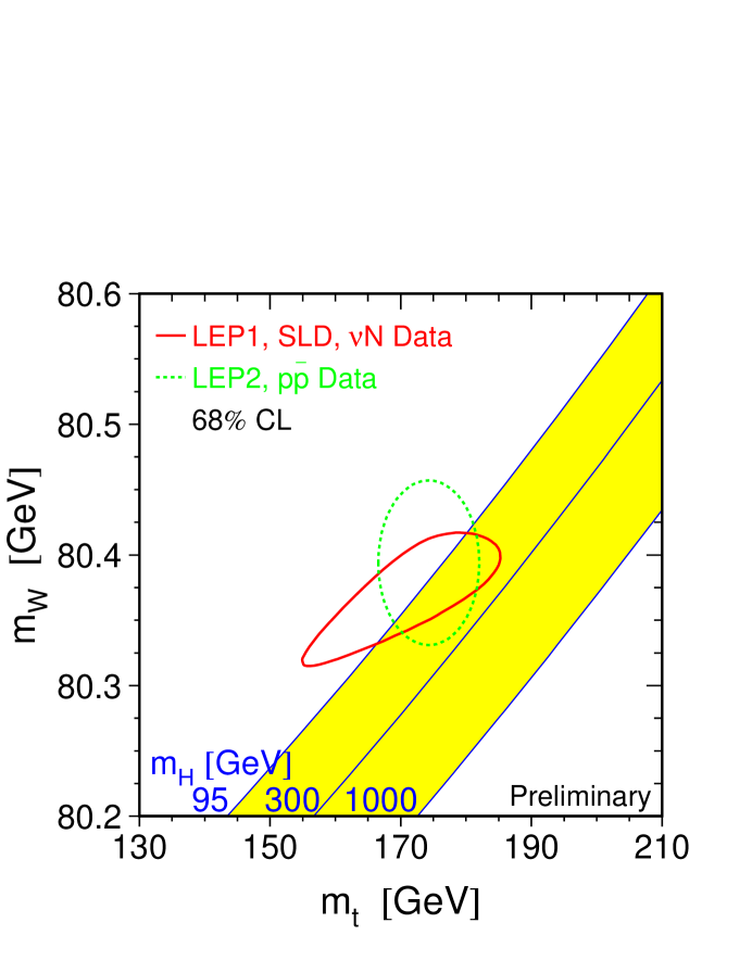
Given this picture of EWSB, the direct and indirect measurements of the top quark and boson masses constrain the mass of the SM Higgs boson (), as indicated in Fig 1. A global fit to all electroweak precision data, including the top quark mass, gives a central value of GeV/c2 and a 95% confidence level upper limit of 225 GeV/c2[1]. In broad classes of SUSY theories the mass of the lightest CP-even neutral Higgs boson, , is constrained to be less than 150 GeV/c2[5]. In the minimal supersymmetric SM (MSSM), the upper bound on is lowered to about 130 GeV/c2[6, 7]. This bound is reasonably robust with respect to changes in the parameters of the theory. Furthermore, in the limit of large pseudo-scalar Higgs boson mass, , where is the mass of the boson, the properties of the lightest MSSM Higgs boson are indistinguishable from those of the SM Higgs boson, . These intriguing indications of a low-mass Higgs boson motivate the study of strategies that maximize the potential for its discovery at the upgraded Tevatron[8]. This paper describes a strategy that achieves this goal.
The current 95% CL lower limit on the Higgs boson mass, from the CERN collider LEP, is 107.9 GeV/c2[9] and is expected to reach close to 114 GeV/c2[7] in the near future. We have therefore studied the mass range 90 GeV/c2 130 GeV/c2, where , hereafter, denotes the SM Higgs boson, . The cross sections for SM Higgs boson production at the Fermilab Tevatron are shown in Fig 2. At TeV, the dominant process for the production of Higgs bosons in collisions is . The Higgs boson decays to a pair about 85% of the time. Unfortunately, even with maximally efficient -tagging this channel is swamped by QCD di-jet production. The more promising channels are , and , which are the ones we have studied.
In events the lepton can be lost because of deficiencies in the detector or the event reconstruction or the lepton energy being below the selection threshold. For such events the reconstructed final state would be indistinguishable from that arising from the process . We have therefore studied these processes in terms of the channels: single lepton ( + + from ), di-lepton ( from ) and missing transverse energy ( + from and ), where denotes the missing transverse energy from all sources, including neutrinos. For each of these channels, we have carried out a comparative study of multivariate and conventional analyses of these channels in which we compare signal significance and the integrated luminosity needed for discovery.
II Optimal Event Selection
In conventional analyses a cut is applied to each event variable, usually one variable at a time, after a visual examination of the signal and background distributions. Although analyses done this way are sometimes described as “optimized,” in practice, unless the signal and background distributions are well separated, the traditional procedure for choosing cuts is rarely optimal in the sense of minimizing the probability to mis-classify events. Since we wish to maximize the chance of discovering the Higgs boson we need to achieve the optimal separation between signal and background, while maximizing the signal significance. Given any set of event variables, optimal separation can always be achieved if one treats the variables in a fully multivariate manner.
Given a set of event variables, it is useful to construct the discriminant function given by
| (1) |
where is the vector of variables that characterize the events and and , respectively, are the dimensional probability densities describing the signal and background distributions. The discriminant function is related to the Bayes discriminant function which is proportional to the likelihood ratio . Working with , instead of directly with , brings two important advantages: 1) it reduces a difficult dimensional optimization problem to a trivial one in a single dimension and 2) a cut on can be shown to be optimal in the sense defined above.
There is, however, a practical difficulty in calculating the discriminant . We usually do not have analytical expressions for the distributions and . What is normally available are large discrete sets of points , generated by Monte Carlo simulations. Fortunately, however, there are several methods available to approximate the discriminant from a set of points , the most convenient of which uses feed-forward neural networks. Neural networks are ideal in this regard because they approximate directly[11, 12].
Many neural network packages are available, any one of which can be used to calculate . We have used the JETNET package[13] to train three-layer (that is, input, hidden and output) feed-forward neural networks (NN). The training was done using the back-propagation algorithm, with the target output for the signal set to one and that for the background set to zero. In this paper we use the terms “neural network output” and “discriminant” interchangeably. However, the distinction between the exact discriminant , as we have defined it above, and the network output, which provides an estimate of , should be borne in mind.
III Single Lepton Channel
We have considered final states with a high electron (e) or muon () and a neutrino from decay and a pair from the decay of the Higgs boson. The events were simulated using the PYTHIA program[14] for Higgs boson masses of = 90, 100, 110, 120 and 130 GeV/c2. In Table I we list the cross section branching ratio (BR) we have used for the process where , .
The processes , , , single top production— and , which have the same signature, , as the signal, are the most important sources of background. They have all been included in our study. The sample was generated using CompHEP[15], a parton level Monte Carlo program based on exact leading order (LO) matrix elements. The parton fragmentation was done using PYTHIA. The single top, and events were simulated using PYTHIA. To generate the s-channel process, , we forced the to be produced off-shell, with , and then selected the final state in which . The cross sections used for the background processes are given in Table I.
To model the expected response of the CDF and DØ Run II detectors at Fermilab we used the SHW program[16], which provides a fast (approximate) simulation of the trigger, tracking, calorimeter clustering, event reconstruction and -tagging. The SHW simulation predicts a di-jet mass resolution of about 14% at = 100 GeV/c2, varying only slightly over the mass range of interest. However, to allow for comparisons with the other and studies at the Physics at Run II SUSY/Higgs workshop[8], some of which do not use SHW, we have re-scaled the di-jet mass variables for all signal and background events so that the resolution is 10% at each Higgs boson mass. The consensus of Run II workshop is that such a mass resolution can be achieved, albeit with considerable effort.
In principle, multivariate methods can be applied at all stages of an analysis. However, in practice, experimental considerations, such as trigger thresholds and the need to restrict data to the phase space in which the detector response is well understood, dictate a set of loose cuts on the event variables. These cuts define a base sample of events. In our case, the base sample was determined by the following cuts:
-
the transverse momentum of the isolated lepton GeV/c
-
the pseudo-rapidity of the lepton
-
the missing transverse energy in the event GeV
-
two or more jets in the event with GeV and .
Since the Higgs decays into a pair we impose the requirement that two jets be -tagged. This of course does little to reduce the dominant background, due to the presence of the pair, but it becomes powerful when the invariant mass, , of the -tagged jets is used as an event variable. The di-jet mass distributions for the signal is expected to peak at the Higgs boson mass, whereas one expects a broad distribution for the background, with the exception of the background which peaks at the boson mass.
One of the -tags was required to be tight and the other loose[16]. A tight -tag is defined by an algorithm that uses the silicon vertex detector, while a loose -tag is defined by the same algorithm with looser cuts or by a soft lepton tag[16]. The mean double -tagging efficiency in SHW is about 45%.
We searched for variables that discriminate between the signal and the backgrounds and arrived at the following set:
-
– transverse energies of the -tagged jets
-
– invariant mass of the -tagged jets
-
– sum of the transverse energies of all selected jets
-
– transverse energy of the lepton
-
– pseudo-rapidity of the lepton
-
– missing transverse energy
-
– sphericity ( where are the eigenvalues obtained by diagonalizing the normalized momentum tensor where the sums are over the final state particle momenta and the subscripts and refer to the spatial components of the momenta
-
– the distance, in the -plane, between the two -tagged jets, where and is the azimuthal angle
-
– the distance between the lepton and the first -tagged jet.
Most of the variables used are directly measured (reconstructed) kinematic quantities while some are deduced variables. The choice of as a discriminating variable is obvious, as discussed earlier. The variable is a measure of the “temperature” of the interaction; a large is a sign of the decay of massive objects. For example, events would have larger (increasing with ) than the background, but smaller than the background. The events are also more spherical than the events and have larger values of sphericity. The is smaller for background where the -jets come mainly from than in events where the -jets come from the heavy object decay .
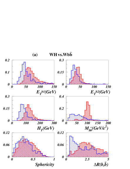
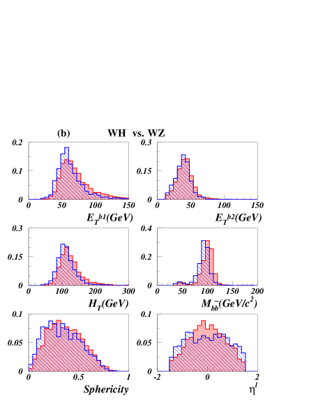
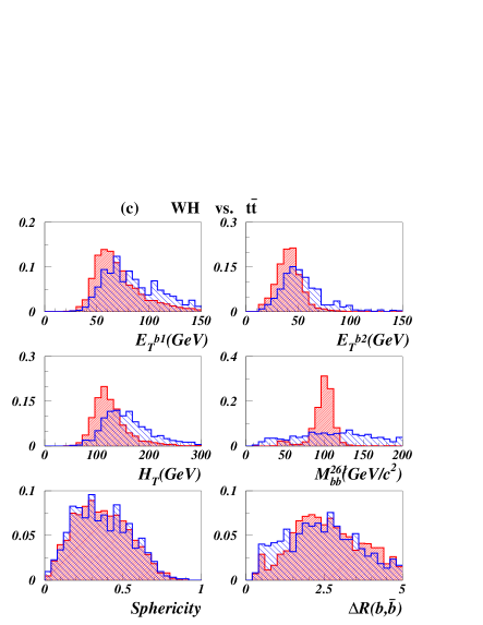
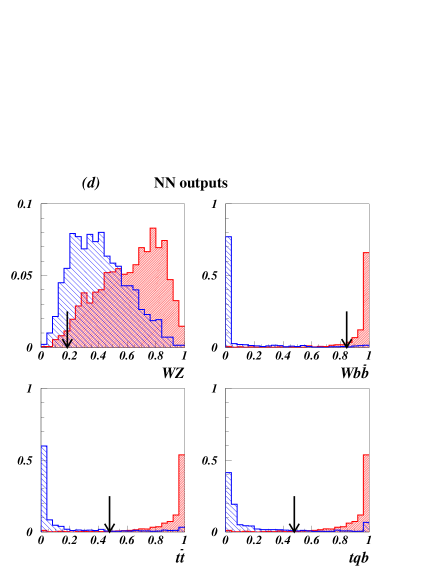
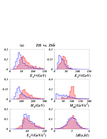
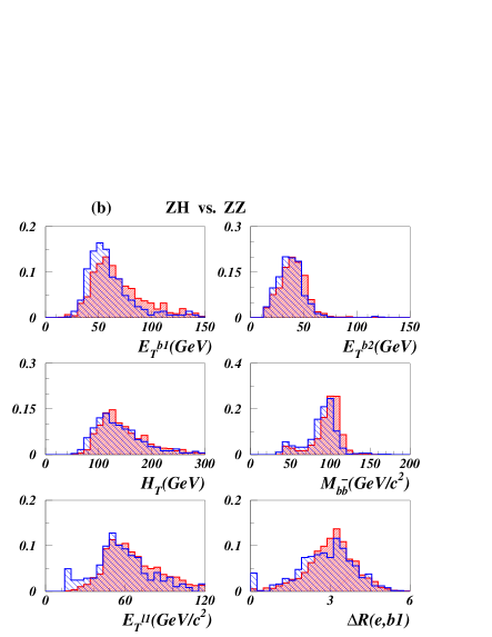
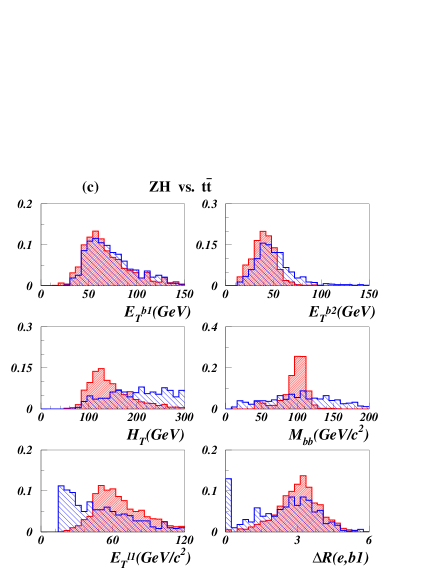
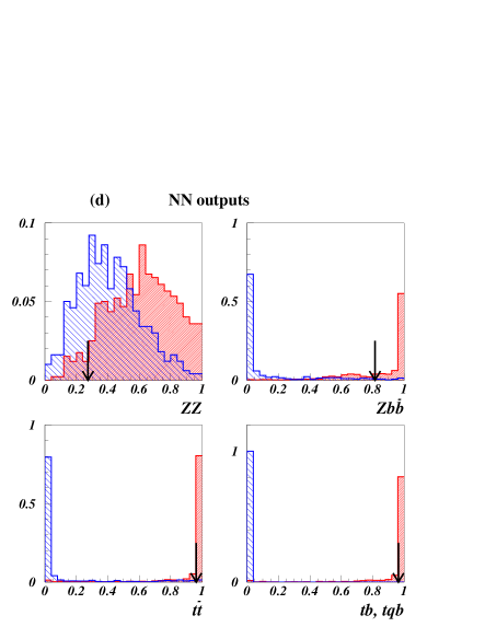
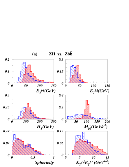
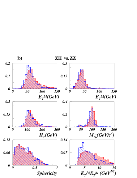
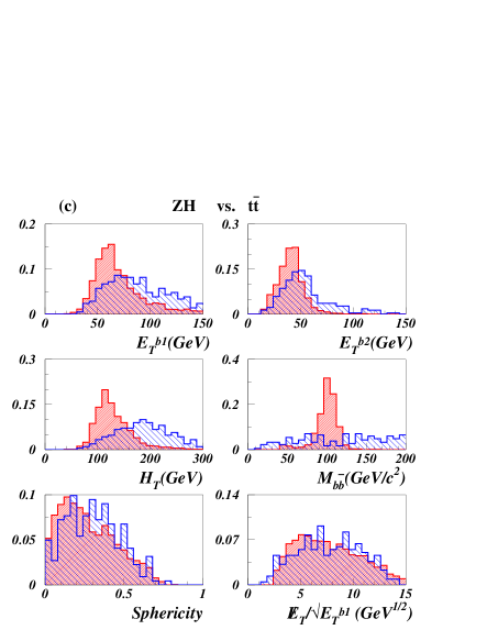
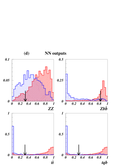
For each Higgs boson mass we trained three networks to discriminate against the main backgrounds , and . The subsets of variables used to train the networks are listed in Table II while in Fig 3(a-c) we show the distributions of some of these variables. Each network has 7 input variables, 9 hidden nodes and one output node. We calcuated three discriminants for every signal and background event and for every Higgs boson mass. Figure 3(d) shows the distributions of the discriminants for signal and background calculated using the network trained to discriminate between signal events, with = 100 GeV/c2, and the specified background. We note that all backgrounds, with the exception of , are well separated from the signal. For Higgs boson masses close to the mass the background is kinematically identical to the signal and therefore difficult to deal with. But for Higgs boson masses well above the mass the discrimination between and improves, as does that between and the other backgrounds. (In all figures, the signal histograms are shaded dark while the background histograms are shaded light.) The arrows in Fig. 3(d) indicate the cuts applied to the discriminants. The cuts were chosen to maximize , where and are the signal and background counts, respectively. The cuts to suppress the background vary from 0.18 to 0.80, increasing for higher Higgs boson masses; the cuts to suppress are generally about 0.8, while those for top events are in the range 0.35 to 0.75.
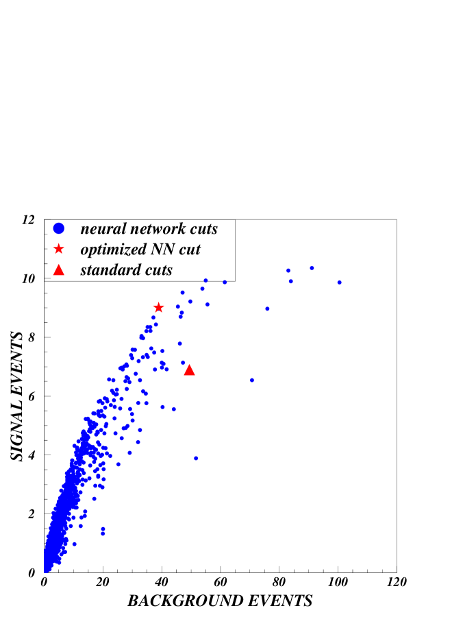
At this stage it is instructive to compare the conventional and multivariate approaches, to assess what has been gained by using the latter approach. In Fig. 4 we compare the signal efficiency vs. background efficiency (given in terms of the number of events for 1 fb-1) for an ensemble of possible cuts on the three discriminants (using the random grid search technique[17]) with the efficiencies obtained using the standard cuts defined by the Run II Higgs Workshop[8]. Each dot corresponds to a particular set of cuts on the three discriminants; the triangular marker indicates what is achieved using the standard cuts, while the star indicates the results obtained from an optimal choice of cuts (which maximizes ) on the three network outputs. Table III shows results for the channel.
IV Di-Lepton Channel
For the di-lepton channel we followed a strategy similar to that described for the single lepton channel. The final state signature considered is: two high same flavor leptons ( or ) from boson decay and two b-jets (from ).
The events were generated using PYTHIA for Higgs boson masses of 90, 100, 110, 120 and 130 GeV/c2. The principal backgrounds are due to , , single top and production. The background sample was generated using CompHEP, with fragmentation done using PYTHIA, while all other samples were generated using PYTHIA. As before, the SHW program was used to simulate the detector response and we assumed that two jets are -tagged (one tight and one loose). The cross sections for signal and background are shown in Table I. The base sample was determined by the following cuts:
-
GeV/c
-
-
GeV
-
at least two jets with GeV and .
A network was trained for each Higgs boson mass and for each of the three backgrounds with the following variables
-
-
of the two leptons
-
-
– invariant mass of the leptons
-
-
between the first lepton and the first -tagged jet.
Distributions of these variables, as well as those of the network output, are shown in Fig 5(a-d). The signal distributions are for =100 GeV/c2. Our results after applying cuts on the three network outputs, for the di-lepton channels are summarized in Table IV.
V Missing Transverse Energy Channel
This channel has contributions from both and where denotes the lepton that is lost. The event generation and detector simulation were carried out as described in the single lepton and di-lepton channel studies. The base sample was defined by the cuts
-
-
GeV/c
-
no isolated lepton with GeV/c
-
GeV
-
at least two jets with GeV and .
The three networks were trained with events as signal and , and as the three backgrounds, respectively. The same networks were used to evaluate contributions from and the relevant backgrounds. We used the following variables to train the networks:
-
-
-
-
-
-
– centrality (, with GeV)
-
-
minimum .
The centrality, , has larger mean value (as is the case with ) for signal events than for backgrounds. The variable is a measure of the significance of the missing transverse energy. The smallest of azimuthal angles between and the jets in the event is expected to be smaller for , as well as high multiplicity events than in signal events. We show the distributions of the variables and neural network outputs in Figs. 6(a-d). Again the signal distributions are for =100 GeV/c2. The results for this channel, after optimized cuts on network outputs, are listed in Table V.
VI Discussion and Summary
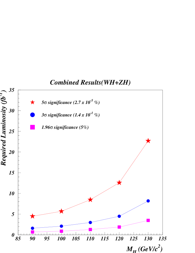
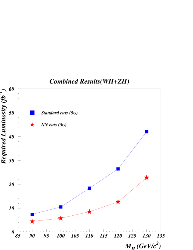
In Table VI we compare the results of our multivariate analysis with those based on the standard cuts, while Table VII and Figs. 7 and 8 show our final results, where we have combined all channels. The striking feature of these results is the substantial reduction in integrated luminosity required to make a discovery of the Higgs boson if one adopts a multivariate approach instead of the traditional method based on univariate cuts. In each of the three channels, the signal significance, which we define as , is seen to be 20-60% higher from our multivariate analysis as compared to an optimal conventional analysis. For example, at GeV/c2 we find that the required integrated luminosity for a observation decreases from 18.3 fb-1 to 8.5 fb-1. The results in Table VII include statistical errors only. The dominant systematic error will likely be due to background modeling. However, given the large data-sets expected by the end of Run II we can anticipate that a thorough experimental study of the relevant backgrounds will have been undertaken. Therefore, it is possible that systematic errors could, eventually, be reduced to well under %. We can estimate the effect of systematic error by adding it in quadrature to the statistical error. If we assume a 10% systematic error on the total background the required integrated luminosity for a observation increases from 8.5 fb-1 to 12.8 fb-1.
Run II at the Tevatron with the CDF and DØ detectors will begin in early 2001. Recently the scope of Run II has been expanded. The goal (hope) is to collect about 15-20 fb-1 per experiment in the period up to and including the start of the LHC. After 5 years of running, each experiment could see a 3-5 signal of a neutral Higgs boson with 130 GeV/c2. This exciting possibility for the Tevatron is the principal motivation for the recent important decision to expand the scope of Run II in order to accumulate as much data as possible. However, even with the expanded scope a discovery may be possible only if these data are analyzed with the most efficient methods available, such as the one we have described in this paper. It is important to note that the results we have presented are for a single experiment. That is, our conclusion is that each experiment has the potential of making an independent discovery. If the experiments combine their results the discovery of a low-mass Higgs boson at the Tevatron might be at hand a lot sooner.
Acknowledgements.
We thank the members of the Run II Higgs Working Group and, in particular, Ela Barberis, Alexander Belyaev, John Conway, John Hobbs, Rick Jesik, Maria Roco and Weiming Yao for useful discussions and for help with the event simulation. The research was supported in part by the U.S. Department of Energy under contract numbers DE-AC02-76CHO3000 and DE-FG02-97ER41022. This work was carried out by the authors as part of the Higgs Working Group***Run II Higgs Working Group (Run II SUSY/Higgs workshop).http://fnth37.fnal.gov/higgs.html. study at Fermilab.
REFERENCES
- [1] J. Erler and P. Langacker, in Proceedings of the 5th International WEIN Symposium: A Conference on Physics Beyond the Standard Model, Santa Fe, NM, 1998; e-print hep-ph/9809352.
- [2] G. Altarelli, CERN report, CERN-TH/97-278; e-print hep-ph/9710434.
- [3] P. C. Bhat, H. B. Prosper and S. S. Snyder, Int. J. Mod. Phys. A13, 5113 (1998).
- [4] LEP Electroweak Group, http://www.cern.ch/LEPEWWG/plots/summer99.
- [5] See for example, S. Martin, in Perspectives on Supersymmetry, edited by G. L. Kane (World Scientific, Singapore, 1998); e-print hep-ph/9709356 v3, 1999.
- [6] M. Carena, M. Quiros, C. E. M. Wagner, Nucl. Phys. B461, 407 (1996).
- [7] B.C. Alanach, et al., Report of the Beyond the Standard Model Working Group of the 1999 UK Phenomenology Workshop on Collider Physics (Durham); e-print hep-ph/9912302.
-
[8]
Run II Higgs Working Group of the Run II SUSY/Higgs workshop.
http://fnth37.fnal.gov/higgs.html; T. Han, A. S. Turcot, and R. Zhang, Phys. Rev. D 59, 093001 (1999). -
[9]
A. Sopczak, e-print hep-ph/0004015, IEKP-KA/2000-06.
See also, http://l3www.cern.ch/conferences/talks99.html. - [10] M. Spira, e-print hep-ph/9810289, A. Djouadi, J. Kalinowski, and M. Spira, e-print hep-ph/9808312.
- [11] P.C. Bhat (for the DØ collaboration), in Proceedings of the 10th Topical Workshop on proton-antiproton Collider Physics, Batavia, IL (AIP, Woodbury, NY, 1995), p. 308; C. M. Bishop, Neural Networks for Pattern Recognition, (Clarendon Press, Oxford, 1998); R. Beale and T. Jackson, Neural Computing: An Introduction, (Adam Hilger, New York, 1991).
- [12] D.W. Ruck et al., IEEE Trans. Neural Networks 1 (4), 296 (1990); E.A. Wan, IEEE Trans. ibid. 1 (4), 303 (1990); E.K. Blum and L.K. Li, Neural Networks, 4, 511 (1991).
- [13] JETNET, C. Peterson, J. Rögnvaldsson, and L. Lönnblad, Comput. Phys. Commun. 81, 185 (1994). We used JETNET version 3.0.
- [14] PYTHIA, T. Sjöstrand, Comput. Phys. Commun. 82, 74 (1994).
- [15] CompHEP, A. S. Belyaev, A.V. Gladyshev and A.V. Semenov, e-print hep-ph/9712303; E.E. Boos et al., e-print hep-ph/9503280.
-
[16]
SHW 2.0,
J. Conway, available at
http://www.physics.rutgers.edu/jconway/soft/shw/shw.html (unpublished). - [17] H. B. Prosper et al., (for the DØ Collaboration), in Proceedings of the International Conference on Computing in High Energy Physics ’95 (Rio de Janeiro, Brazil) (World Scientific, River Edge, NJ, 1996).
| (GeV/c2) | (GeV/c2) | (GeV/c2) | |||
| 90 | 119.0 | 90 | 20.3 | 90 | 40.6 |
| 100 | 85.4 | 100 | 14.8 | 100 | 29.6 |
| 110 | 62.3 | 110 | 10.9 | 110 | 21.8 |
| 120 | 45.3 | 120 | 8.22 | 120 | 16.4 |
| 130 | 34.1 | 130 | 6.25 | 130 | 12.5 |
| Backgrounds | |||||
| 3500.0 | 350.0 | 700.0 | |||
| 164.8 | |||||
| 800.0 | 800.0 | 800.0 | |||
| (fb) | (fb) | (fb) | |||
| 1235.0 | 1235.0 | ||||
| 1000.0 | 1000.0 | 1000.0 | |||
| 7500.0 | 7500.0 | 7500.0 | |||
| GeV/c2 | 90 | 100 | 110 | 120 | 130 |
|---|---|---|---|---|---|
| Number of events(1 fb-1) | |||||
| 8.65 | 8.97 | 4.81 | 4.41 | 3.71 | |
| 12.28 | 12.48 | 5.84 | 9.66 | 20.12 | |
| 7.52 | 10.32 | 1.72 | 1.00 | 0.97 | |
| 0.51 | 0.95 | 0.58 | 0.71 | 0.96 | |
| 2.46 | 5.40 | 3.44 | 5.89 | 9.33 | |
| 5.63 | 9.89 | 7.24 | 8.39 | 14.49 | |
| Total background | 28.40 | 39.04 | 18.81 | 25.67 | 45.87 |
| Signal significance | |||||
| S/B | 0.31 | 0.23 | 0.26 | 0.17 | 0.081 |
| S/ (1 fb-1) | 1.62 | 1.44 | 1.11 | 0.87 | 0.55 |
| S/ (2 fb-1) | 2.29 | 2.04 | 1.57 | 1.23 | 0.78 |
| S/ (30 fb-1) | 8.87 | 7.89 | 6.08 | 4.77 | 3.01 |
| Required luminosity (fb-1) | |||||
| 9.5 | 12.1 | 20.3 | 33.0 | 82.6 | |
| 3.4 | 4.3 | 7.3 | 11.9 | 29.8 | |
| (95% CL) | 1.5 | 1.9 | 3.1 | 5.1 | 12.7 |
| (GeV/c2) | 90 | 100 | 110 | 120 | 130 |
|---|---|---|---|---|---|
| Number of events | |||||
| 1.26 | 0.87 | 0.79 | 0.80 | 0.58 | |
| 0.61 | 0.45 | 0.61 | 1.50 | 1.42 | |
| 2.04 | 1.44 | 1.42 | 0.83 | 0.31 | |
| 0.28 | 0.05 | 0.23 | 0.44 | 0.18 | |
| Total background | 2.93 | 1.94 | 2.26 | 2.77 | 1.91 |
| 0.43 | 0.45 | 0.35 | 0.29 | 0.31 | |
| 0.74 | 0.63 | 0.54 | 0.48 | 0.42 |
| (GeV/c2) | 90 | 100 | 110 | 120 | 130 |
|---|---|---|---|---|---|
| Number of events | |||||
| 6.66 | 4.37 | 3.53 | 2.76 | 2.16 | |
| 5.59 | 3.75 | 2.79 | 1.98 | 1.70 | |
| Total signal | 12.25 | 8.12 | 6.32 | 4.74 | 3.86 |
| 8.12 | 4.97 | 4.83 | 3.85 | 3.92 | |
| 21.70 | 13.12 | 10.68 | 8.22 | 7.53 | |
| 11.24 | 6.14 | 2.59 | 1.05 | 0.59 | |
| 7.95 | 4.49 | 1.99 | 0.90 | 0.54 | |
| 0.63 | 0.27 | 0.37 | 0.24 | 0.29 | |
| 6.83 | 2.99 | 4.27 | 5.12 | 6.40 | |
| 5.10 | 2.70 | 3.00 | 3.00 | 4.35 | |
| Total background | 61.57 | 34.8 | 27.73 | 22.38 | 23.62 |
| 0.20 | 0.23 | 0.23 | 0.21 | 0.16 | |
| 1.56 | 1.38 | 1.20 | 1.00 | 0.79 |
| channel | mass | standard | neural | / |
|---|---|---|---|---|
| (GeV) | cuts | net | (for obsv.) | |
| 100 | 0.98 | 1.44 | 0.46 | |
| 110 | 0.69 | 1.11 | 0.39 | |
| 120 | 0.58 | 0.87 | 0.44 | |
| 130 | 0.44 | 0.55 | 0.64 | |
| 100 | 1.09 | 1.38 | 0.62 | |
| 110 | 0.85 | 1.20 | 0.50 | |
| 120 | 0.67 | 1.00 | 0.49 | |
| 130 | 0.54 | 0.78 | 0.47 | |
| 100 | 0.48 | 0.63 | 0.58 | |
| 110 | 0.40 | 0.52 | 0.59 | |
| 120 | 0.40 | 0.48 | 0.69 | |
| 130 | 0.33 | 0.42 | 0.61 |
| (GeV/c2) | 90 | 100 | 110 | 120 | 130 |
|---|---|---|---|---|---|
| (1 fb-1) | 2.4 | 2.1 | 1.7 | 1.4 | 1.0 |
| (2 fb-1) | 3.3 | 3.0 | 2.4 | 2.0 | 1.5 |
| (30 fb-1) | 12.9 | 11.5 | 9.4 | 7.7 | 5.7 |
| Required luminosity | |||||
| (Conventional) | 7.5 | 10.5 | 18.3 | 26.6 | 42.2 |
| (NN) | 4.5 | 5.7 | 8.5 | 12.6 | 22.7 |
| (NN) | 1.6 | 2.1 | 3.0 | 4.5 | 8.2 |
| 95% CL (NN) | 0.7 | 0.9 | 1.3 | 1.9 | 3.5 |