Chiral Gauge Theory on Lattice with Domain Wall Fermions

Abstract

We investigate a $U(1)$ lattice chiral gauge theory ($L\chi GT$) with domain wall fermions and compact gauge fixing. In the reduced model limit, our perturbative and numerical investigations show that there exist no extra mirror chiral modes. The longitudinal gauge degrees of freedom have no effect on the free domain wall fermion spectrum consisting of opposite chiral modes at the domain wall and at the anti-domain wall which have an exponentially damped overlap.

I Introduction

Lattice regularization of chiral gauge theories has remained a long standing problem of nonperturbative investigation of quantum field theory. Lack of chiral gauge invariance in $L\chi GT$ proposals is responsible for the longitudinal gauge degrees of freedom (dof) coupling to fermionic dof and eventually spoiling the chiral nature of the theory. The well-known example is the Smit-Swift proposal of $L\chi GT$ [2]. Although in a recent development using a Dirac operator that satisfies the Ginsparg-Wilson relation, it was possible to formulate a $L\chi GT$ without violating gauge-invariance or locality [3], an explicit model for nonperturbative numerical studies is still not available.

In this paper, we follow the gauge fixing approach to $L\chi GT$ [4]. The obvious remedy to control the longitudinal gauge dof is to gauge fix with a target theory in mind. The Roma proposal [5] involving gauge fixing passed perturbative tests but does not address the problem of gauge fixing of compact gauge fields and the associated problem of lattice artifact Gribov copies. The formal problem is that for compact gauge fixing a BRST-invariant partition function as well as (unnormalized) expectation values of BRST invariant operators vanish as a consequence of lattice Gribov copies [6]. Shamir and Golterman [4] have proposed to keep the gauge fixing part of the action BRST noninvariant and tune counterterms to recover BRST in the continuum. In their formalism, the continuum limit is to be taken from within the broken ferromagnetic (FM) phase approaching another broken phase which is called ferromagnetic directional (FMD) phase, with the mass of the gauge field vanishing at the FM-FMD transition. This was tried out in a $U(1)$ Smit-Swift model and so far the results show that in the pure gauge sector, QED is recovered in the continuum limit [7] and in the reduced model limit (to be defined below) free chiral fermions in the appropriate chiral representation are obtained [8]. Tuning with counterterms has also not posed any practical problem, actually very little tuning is necessary. Efforts are currently underway to extend this gauge fixing proposal to include nonabelian gauge groups [9].

Without gauge fixing the longitudinal gauge dof, which are radially frozen scalar fields, are rough and nonperturbative even if the transverse gauge coupling may be weak (this is because with the standard lattice measure, each point on the gauge orbit has equal weight). The theory in the continuum limit, taken at the transition between the broken symmetry ferromagnetic (FM) phase and the symmetric paramagnetic (PM) phase, displays undesired nonperturbative effects of the scalar-fermion coupling that usually spells disaster for the chiral theory. The job of the gauge fixing is to introduce a new continuous phase transition, from the FM phase to a new broken symmetry phase (FMD), at which the gauge symmetry is recovered and at the same time the gauge fields become smooth.

The problem can be cleanly studied in the reduced model as explained in the following. When one gauge transforms a gauge non-invariant theory, one picks up the longitudinal gauge degrees of freedom (radially frozen scalars) explicitly in the action. The reduced model is then obtained by making the lattice gauge field unity for all links, i.e., by switching off the transverse gauge coupling. The action becomes that of a chiral Yukawa theory with interaction between the fermions and the longitudinal gauge dof. The reduced model would have a phase structure similar to the full theory, e.g., the gauge fixed theory in the reduced limit will have a FM-FMD transition in addition to the FM-PM transition. Now for the gauge fixing proposal to work, the scalars need to decouple from the fermions at the FM-FMD transition leaving the fermions free in the appropriate chiral representation. Passing the reduced model test is an important first step for any $L\chi GT$ proposal that breaks gauge invariance.

In the reduced model derived from the gauge fixed theory the scalar fields become smooth and expandable in a perturbative series as $1+{\cal O}(\mbox{coupling constant})$ at the FM-FMD transition. If continuum limit can be taken near the point in the coupling parameter space around which this perturbative expansion is defined, the scalar fields will decouple from the theory. The parameterization of the gauge fixing action turns out to be a good one, because this continuum limit can be taken ($i$) very easily by approaching the FM-FMD transition almost perpendicularly by tuning essentially one counterterm, and ($ii$) at a point on this transition line which is reasonably far away from the expansion point. This has been possible in [8] and again in the present work.

A central claim of the gauge fixing proposal is that it is universal, i.e., it should work with any lattice fermion action that has the correct classical continuum limit. This is because the central idea as discussed above is independent of the particular lattice fermion regularization. In the present paper we want to confirm the universality claim by applying the proposal to domain wall fermions [10] with $U(1)$ gauge group. For this purpose we have chosen the waveguide formulation [11] of the domain wall fermion and investigate in the reduced model. This model was investigated before without gauge fixing and the free domain wall spectrum was not obtained in the reduced limit [12]. Mirror chiral modes were found at the waveguide boundaries in addition to the chiral modes at the domain wall or anti-domain wall.

In section II we present the gauge-fixed domain wall fermion action for a $U(1)$ chiral gauge theory and then go to the so-called reduced model by switching off the transverse gauge coupling. In section III we perform a weak coupling perturbation theory in the reduced model for the fermion propagators and mass matrix to 1-loop. However, in sections III C and III D we have used special boundary conditions (instead of the actual Kaplan boundary conditions) to arrive at explicit expressions for the overlap of the opposite chiral modes. Our numerical results for the quenched phase diagram and chiral fermion propagators at the domain wall and anti-domain wall and at the waveguide boundaries are presented and compared with the perturbative results in section IV. We summarize in the concluding section V. In Appendix A, we describe the special boundary conditions used in sections III C and III D. In Appendix B we schematically discuss how using Kaplan boundary conditions one can arrive at the same qualitative conclusion about the 1-loop overlap of the opposite chiral modes.

II Gauge-fixed Domain Wall Action

Kaplan’s free domain wall fermion action [10] on a $4+1$-dimensional lattice is given by (lattice constant is taken to be unity throughout this paper),

$$S_{F}=\sum_{XY}\overline{\psi}_{X}\left[\partial\!\!\!/_{5}-w_{5}+{\bf M}\right]_{XY}\psi_{Y}$$ (1)

where $\overline{\psi}$ and $\psi$ are the fermion fields, and $\partial\!\!\!/_{5}$ and $w_{5}$ are respectively the 5-dimensional Dirac operator and the Wilson term,

$$(\partial\!\!\!/_{5})_{XY} = \frac{1}{2}\sum_{\alpha=1}^{5}\gamma_{\alpha}\left(\delta_{X+\hat{\alpha},Y}-\delta_{X-\hat{\alpha},Y}\right),$$ (2)

$$(w_{5})_{XY} = \frac{r}{2}\sum_{\alpha=1}^{5}\left(\delta_{X+\hat{\alpha},Y}+\delta_{X-\hat{\alpha},Y}-2\delta_{XY}\right),$$ (3)

The $\gamma_{\alpha}$’s are the five hermitian euclidean gamma matrices, $r$ is the Wilson parameter, $X=(x,s),~{}Y=(y,t)$ label the sites of the $L^{4}L_{s}$ lattice and $L_{s}$ is the extent of the 5th dimension: $0\leq s,t\leq L_{s}-1$. We are interested in taking the continuum limit in the 4 space-time dimensions only. It is convenient to look at the 5-th dimension as a flavor space.

With periodic boundary conditions in the 5th or $s$-direction ($s,t=L_{s}\Rightarrow s,t=0$) and the domain wall mass ${\bf M}$ taken as

$${\bf M}_{XY}=m(s)\delta_{XY},\;\;{\rm where},$$ (4)

$$m(s)=\begin{array}[]{rl}-m_{0},&0<s<L_{s}/2\\ 0,&s=0,L_{s}/2\\ m_{0},&L_{s}/2<s<L_{s}\end{array}$$ (5)

the model possesses a lefthanded (LH) chiral mode bound to the domain wall at $s=0$ and a righthanded (RH) chiral mode bound to the anti-domain wall at $s=L_{s}/2$. For $m_{0}L_{s}\gg 1$, these modes have exponentially small overlap. The chiral modes exist for momenta $p$ below a critical momentum $p_{c}$, i.e. $|\hat{p}|<p_{c}$, where $\hat{p}^{2}=2\sum_{\mu}[1-\cos(p_{\mu})]$ and $p_{c}^{2}=4-2m_{0}/r$. Taking the Wilson parameter $r=1$ the choice of $m_{0}$ is then restricted to $0<m_{0}<2$.

A 4-dimensional gauge field which is same for all $s$-slices can be coupled to fermions only for a restricted number of $s$-slices around the anti-domain wall [12] with a view to coupling only to the RH mode at the anti-domain wall. The gauge field is thus confined within a waveguide,

$$WG = (s:s_{0}<s\leq s_{1})$$ (6)

$${\rm with}\hskip 14.22636pts_{0} = \frac{L_{s}+2}{4}-1,\hskip 19.91684pts_{1}=\frac{3L_{s}+2}{4}-1.$$ (7)

With this choice, $(L_{s}-2)$ has to be a multiple of 4. For convenience, the boundaries at ($s_{0},s_{0}+1$) and ($s_{1},s_{1}+1$) are denoted waveguide boundary $I$ and $II$ respectively.

The gauge transformations on the fermion fields are defined as follows:

$$\psi_{x}^{s}\rightarrow g_{x}\psi_{x}^{s},\hskip 22.76228pt \overline{\psi}_{x}^{s} \rightarrow\overline{\psi}_{x}^{s}g_{x}^{\dagger}\hskip 22.76228pts\in WG$$ (8)

$$\psi_{x}^{s}\rightarrow\psi_{x}^{s},\hskip 22.76228pt \overline{\psi}_{x}^{s} \rightarrow\overline{\psi}_{x}^{s}\hskip 32.72049pts\in\!\!\!\!\!/\;WG$$ (9)

where $g_{x}\in G$, the gauge group. Other symmetries of the model remain the same as in [12].

Obviously, the hopping terms from $s_{0}$ to $s_{0}+1$ and that from $s_{1}$ to $s_{1}+1$ would break the local gauge invariance of the action. This is taken care of by gauge transforming the action and thereby picking up the pure gauge dof or a radially frozen scalar field $\varphi$ (Stückelberg field) at the waveguide boundary, leading to the gauge-invariant action (with $\varphi_{x}\rightarrow g_{x}\varphi_{x}$ and (9)) :

$$S_{F} = \sum_{s\in WG}\overline{\psi}^{s}\left(D\!\!\!\!/\,(U)-W(U)+m(s)\right)\psi^{s}+\sum_{s\not\in WG}\overline{\psi}^{s}\left(\partial\!\!\!/-w+m(s)\right)\psi^{s}$$ (10)

$$+ \;\sum_{s}\overline{\psi}^{s}\psi^{s}-\sum_{s\neq s_{0},s_{1}}\left(\overline{\psi}^{s}P_{L}\psi^{s+1}+\overline{\psi}^{s+1}P_{R}\psi^{s}\right)$$ (11)

$$- \;y\left(\overline{\psi}^{s_{0}}\varphi^{\dagger}P_{L}\psi^{s_{0}+1}+\overline{\psi}^{s_{0}+1}\varphi P_{R}\psi^{s_{0}}\right)-y\left(\overline{\psi}^{s_{1}}\varphi P_{L}\psi^{s_{1}+1}+\overline{\psi}^{s_{1}+1}\varphi^{\dagger}P_{R}\psi^{s_{1}}\right)$$ (12)

where we have taken the Wilson parameter $r=1$ and have suppressed all indices other than $s$. The projector $P_{L(R)}$ is $(1\mp\gamma_{5})/2$ and $y$ is the Yukawa coupling introduced by hand at the waveguide boundaries. $D\!\!\!\!/\;(U)$ and $W(U)$ are respectively the gauge covariant Dirac operator and the Wilson term in 4 space-time dimensions. $\partial\!\!\!/$ and $w$ are the 4-dimensional versions of (3).

The gauge-fixed pure gauge action for $U(1)$, where the ghosts are free and decoupled, is:

$$S_{B}(U)=S_{g}(U)+S_{gf}(U)+S_{ct}(U)$$ (13)

where, $S_{g}$ is the usual Wilson plaquette action; the gauge fixing term $S_{gf}$ (as proposed by Shamir and Golterman) and the gauge field mass counter term $S_{ct}$ are given by (for a discussion of relevant counterterms see [4, 13]),

$$S_{gf}(U) = \tilde{\kappa}\left(\sum_{xyz}\Box(U)_{xy}\Box(U)_{yz}-\sum_{x}B_{x}^{2}\right),$$ (14)

$$S_{ct}(U) = -\kappa\sum_{x\mu}\left(U_{\mu x}+U_{\mu x}^{\dagger}\right),$$ (15)

where $\Box(U)$ is the covariant lattice laplacian and

$$B_{x}=\sum_{\mu}\left(\frac{V_{\mu x-\hat{\mu}}+V_{\mu x}}{2}\right)^{2}$$ (16)

with $V_{\mu x}=\frac{1}{2i}\left(U_{\mu x}-U_{\mu x}^{\dagger}\right)$ and $\tilde{\kappa}=1/(2\xi g^{2})$.

$S_{gf}$ is not just a naive lattice transcription of the continuum covariant gauge fixing term, it has in addition appropriate irrelevant terms. As a result, $S_{gf}$ has a unique absolute minimum at $U_{\mu x}=1$, validating weak coupling perturbation theory (WCPT) around $g=0$ or $\tilde{\kappa}=\infty$ and in the naive continuum limit it reduces to $\frac{1}{2\xi}\int d^{4}x(\partial_{\mu}A_{\mu})^{2}$.

Obviously, the action $S_{B}(U)$ is not gauge invariant. By giving it a gauge transformation the resulting action $S_{B}(\varphi^{\dagger}_{x}U_{\mu x}\varphi_{x+\hat{\mu}})$ is gauge-invariant with $U_{\mu x}\rightarrow g_{x}U_{\mu x}g^{\dagger}_{x+\hat{\mu}}$ and $\varphi_{x}\rightarrow g_{x}\varphi_{x}$, $g_{x}\in U(1)$. By restricting to the trivial orbit, we arrive at the so-called reduced model action

$$S_{reduced}=S_{F}(U=1)+S_{B}(\varphi^{\dagger}_{x}\;1\;\;\varphi_{x+\hat{\mu}})$$ (17)

where $S_{F}(U=1)$ is obtained quite easily from eq.(12) and

$$S_{B}(\varphi^{\dagger}_{x}\;1\;\;\varphi_{x+\hat{\mu}})=-\kappa\sum_{x}\varphi^{\dagger}_{x}(\Box\varphi)_{x}+\tilde{\kappa}\sum_{x}\left[\varphi^{\dagger}_{x}(\Box^{2}\varphi)_{x}-B^{2}_{x}\right]$$ (18)

now is a higher-derivative scalar field theory action. $B_{x}$ in (18) is same as in (16) with

$$V_{\mu x}=\frac{1}{2i}\left(\varphi^{\dagger}_{x}\varphi_{x+\hat{\mu}}-\varphi^{\dagger}_{x+\hat{\mu}}\varphi_{x}\right).$$ (19)

In the following, we investigate the action (17) at $y=1$ by analytical and numerical methods. Some numerical results with other values of $y$ have been presented in [14]. The waveguide model strictly at $y=0$ would give rise to opposite chiral modes at the waveguide boundaries as can be seen from fermion current considerations [12] (and also from numerical simulation) and would thereby spoil the chiral nature of the theory. It is an interesting question to investigate the model for $0<y<1$. Analysis of the results for small values of $y(<1)$ is tricky and will be discussed in a separate article [15].

III Weak Coupling Perturbation Theory in the Reduced Model

At $y=1$, we carry out a WCPT in the coupling $1/\tilde{\kappa}$ for the fermion propagators to 1-loop. In order to develop perturbation theory, in reduced model, we expand,

$$\varphi_{x}=\exp(ib\theta_{x})=1+ib\theta_{x}-\frac{1}{2}b^{2}\theta_{x}^{2}+{\cal O}(b^{3})$$ (20)

where, $b=1/\sqrt{2\tilde{\kappa}}$ and $\theta_{x}$ is dimensionless, leading to

$$S=S_{F}^{(0)}(\psi,\overline{\psi};y)+S_{B}^{(0)}(\theta)+S^{({\rm int})}(\psi,\overline{\psi},\theta;y)$$ (21)

where $S^{(0)}$’s are free actions and $S^{({\rm int})}$ is the interaction part.

A Scalar propagator at tree level

From $S_{B}^{(0)}(\theta)$ one gets the free propagator for the compact scalar $\theta$ [13],

$${\cal G}(k)=\frac{1}{\hat{k^{2}}(\hat{k^{2}}+\omega^{2})},\hskip 28.45274pt\omega^{2}=\frac{\kappa}{\tilde{\kappa}}$$ (22)

where, $\hat{k}_{\mu}=2\sin(k_{\mu}/2)$.

B $LL$ and $RR$ fermion propagators at tree level and at 1-loop

1 Tree level

With $y=1$, $S_{F}^{(0)}(\psi,\overline{\psi};y=1)$ is the free domain wall action (1). Free fermion propagators at $y=1$ are obtained in momentum space for 4-spacetime dimensions while staying in the coordinate space for the 5th dimension following [16] (results in [16, 17, 18] cannot be directly used because of difference in implementation of the domain wall (5)). The free action is written as,

$$S_{F}^{(0)}(y=1)=\sum_{p,s,t}\overline{\widetilde{\psi_{p}^{s}}}\left[i\overline{p\!\!\!/}\delta_{s,t}+M_{st}P_{L}+M^{\dagger}_{st}P_{R}\right]\widetilde{\psi_{p}^{t}}$$ (23)

where, $M_{st}=F(p)\delta_{s,t}+(M_{0})_{st}$, $(M_{0})_{st}=[1+m(s)]\delta_{s,t}-\delta_{s+1,t}$, $F(p)=\sum_{\mu}(1-\cos(p_{\mu}))$, $\overline{p}_{\mu}=\sin(p_{\mu})$ and $\overline{p\!\!\!/}=\gamma_{\mu}\overline{p}_{\mu}$. The free fermion propagator can formally be written as,

$$\Delta(p) = \left[i\overline{p\!\!\!/}+MP_{L}+M^{\dagger}P_{R}\right]^{-1}$$ (24)

$$= (-i\overline{p\!\!\!/}+M^{\dagger})P_{L}G_{L}(p)+(-i\overline{p\!\!\!/}+M)P_{R}G_{R}(p)$$ (25)

where,

$$G_{L}(p) = \frac{1}{\sum_{\mu}\overline{p}_{\mu}^{2}+MM^{\dagger}}$$ (26)

$$G_{R}(p) = \frac{1}{\sum_{\mu}\overline{p}_{\mu}^{2}+M^{\dagger}M}.$$ (27)

Solution of $G_{L}$ is obtained by writing (26) explicitly:

$$\left[\overline{p}^{2}+1+B(s)^{2}\right](G_{L})_{s,t}-B(s+1)(G_{L})_{s+1,t}-B(s)(G_{L})_{s-1,t}=\delta_{s,t}$$ (28)

and similarly for $G_{R}$. In (28), $B(s)=F(p)+1+m(s)$. We show only the calculations for obtaining $G_{L}$ and henceforth drop the subscript $L$.

Setting the notation as follows:

$$G = G^{-},\;\;\;\;B(s)=F(p)+1-m_{0}=a_{-}\hskip 22.76228pt{\rm for}\;\;\;\;0<s\leq L_{s}/2-1$$ (29)

$${\rm and}\hskip 11.38092ptG = G^{+},\;\;\;\;B(s)=F(p)+1+m_{0}=a_{+}\hskip 22.76228pt{\rm for}\;\;\;\;L_{s}/2<s\leq L_{s}-1,$$ (30)

the equations for $G^{\pm}$ are given by,

$$\left(\overline{p}^{2}+1+a^{2}_{-}\right)G^{-}_{s,t}-a_{-}G^{-}_{s+1,t}-a_{-}G^{-}_{s-1,t} = \delta_{s,t},$$ (31)

$$\left(\overline{p}^{2}+1+a^{2}_{+}\right)G^{+}_{s,t}-a_{+}G^{+}_{s+1,t}-a_{+}G^{+}_{s-1,t} = \delta_{s,t}.$$ (32)

The ranges of $s$ in eqs.(29, 30) for which $G^{-}$ and $G^{+}$ are defined, are applicable only to the translationally invariant eqs.(31, 32). In general for the translationally noninvariant eq.(28) we also define $G^{-}$ and $G^{+}$ at $s=0$ and $L_{s}/2$, the ones excluded by (31, 32). The $\pm$ superscript to $G$ at $s=0,\;L_{s}/2$ is decided by the translationally invariant $s$-sector from which $s=0$ or $L_{s}/2$ is approached in eq.(28). We have used this notation for the boundary conditions eq.(38) below.

The solutions of the eqs.(31, 32) are expressed as sum of homogeneous and inhomogeneous solutions:

$$G^{\pm}_{s,t}(p)=g_{\pm}^{(1)}(t)e^{-\alpha_{\pm}(p)s}+g_{\pm}^{(2)}(t)e^{\alpha_{\pm}(p)s}+\frac{\cosh[\alpha_{\pm}(p)(|s-t|-l/2)]}{2a_{\pm}\sinh(\alpha_{\pm}(p))\sinh(\alpha_{\pm}(p)l/2)},$$ (33)

where, $l=L_{s}/2$ and

$$\cosh(\alpha_{\pm}(p))=\frac{1}{2}\left(a_{\pm}+\frac{1+\overline{p}^{2}}{a_{\pm}}\right).$$ (34)

The third term in (33) is the inhomogeneous solution. To avoid singularities in $\alpha_{\pm}(p)$ when $a_{\pm}$ is zero further restricts the allowed range of $m_{0}$ to $0<m_{0}<1$. In this paper we have taken $m_{0}=0.5$.

In order to get the complete solution we need to determine the unknown functions $g_{\pm}^{(1)}(t)$ and $g_{\pm}^{(2)}(t)$ in (33), which are obtained by considering boundary conditions from eqs.(31, 32) at $s=0,\;1,\;L_{s}/2-1,\;L_{s}/2,\;L_{s}/2+1,\;L_{s}-1$,

$$a_{0}G^{-}_{0,t}(p) = a_{+}G^{+}_{L_{s},t}(p),$$ (35)

$$a_{0}G^{+}_{L_{s}/2,t}(p) = a_{-}G^{-}_{L_{s}/2,t}(p),$$ (36)

$$(\overline{p}^{2}+1+a_{0}^{2})G^{-}_{0,t}(p)-a_{-}G^{-}_{1,t}(p) = \delta_{0,t}+a_{0}G^{+}_{L_{s}-1,t}(p),$$ (37)

$$(\overline{p}^{2}+1+a_{0}^{2})G^{+}_{L_{s}/2,t}(p)-a_{+}G^{+}_{L_{s}/2+1,t} = \delta_{L_{s}/2,t}+a_{0}G^{-}_{L_{s}/2-1,t}.$$ (38)

with $B(s)=F(p)+1=a_{0}$ at $s=0,L_{s}/2$. It is to be noted that these boundary conditions are significantly different from the ones given in [16] because of the difference in implementation of the domain wall. $G^{-}_{0,t}$ and $G^{+}_{L_{s}/2,t}$ (and the corresponding ones from $G_{R}$) are used to determine the free chiral propagators at the domain wall and anti-domain wall for comparison with numerical data in Fig.4. We will see later that these chiral propagators do not receive any 1-loop self-energy corrections.

Substituting $\overline{p}^{2}+1+a_{0}^{2}=F_{0}$ and $2a_{\pm}\sinh(\alpha_{\pm}(p))\sinh(\alpha_{\pm}(p)l/2)=X_{\pm}$ and using the boundary conditions, eqs.(38), we arrive at an equation of the form,

$${\bf A}\cdot{\bf g}(t)={\bf X}(t),$$ (39)

where, ${\bf g}(t)=(g_{-}^{(1)}\;\;\;g_{-}^{(2)}\;\;\;g_{+}^{(1)}\;\;\;g_{+}^{(2)})$ is a 4-component vector, ${\bf X}(t)$ is another 4-component vector and ${\bf A}$ is a $4\times 4$ matrix as given below,

$\displaystyle{\bf A}=\left(\begin{array}[]{cccc}a_{0}&a_{0}&-a_{+}e^{-\alpha_{+}L_{s}}&-a_{+}e^{\alpha_{+}L_{s}}\\ a_{-}e^{-\alpha_{-}L_{s}/2}&a_{-}e^{\alpha_{-}L_{s}/2}&-a_{0}e^{-\alpha_{+}L_{s}/2}&-a_{0}e^{\alpha_{+}L_{s}/2}\\ F_{0}-a_{-}e^{-\alpha_{-}}&F_{0}-a_{-}e^{\alpha_{-}}&-a_{0}e^{-\alpha_{+}(L_{s}-1)}&-a_{0}e^{\alpha_{+}(L_{s}-1)}\\ -a_{0}e^{-\alpha_{-}(L_{s}/2-1)}&-a_{0}e^{\alpha_{-}(L_{s}/2-1)}&(F_{0}-a_{+}e^{-\alpha_{+}})e^{-\alpha_{+}L_{s}/2}&(F_{0}-a_{+}e^{\alpha_{+}})e^{\alpha_{+}L_{s}/2}\end{array}\right)$

and

$\displaystyle{\bf X}(t)=\left(\begin{array}[]{ll}a_{+}X_{+}\cosh[\alpha_{+}(|L_{s}-t|-l/2)]&-\,a_{0}X_{-}\cosh[\alpha_{-}(|-t|-l/2)]\\ &\\ a_{0}X_{+}\cosh[\alpha_{+}(|L_{s}/2-t|-l/2)]&-\,a_{-}X_{-}\cosh[\alpha_{-}(|L_{s}/2-t|-l/2)]\\ &\\ \delta_{0,t}+a_{0}X_{+}\cosh[\alpha_{+}(|L_{s}-1-t|\,-&l/2)]-F_{0}X_{-}\cosh[\alpha_{-}(|-t|-l/2)]+\\ &\hskip 99.58464pta_{-}X_{-}\cosh[\alpha_{-}(|1-t|-l/2)]\\ &\\ \delta_{L_{s}/2,t}+a_{+}X_{+}\cosh[\alpha_{+}(|L_{s}/2+1-&\!\!t|-l/2)]-F_{0}X_{+}\cosh[\alpha_{+}(|L_{s}/2-t|-l/2)]+\\ &\hskip 68.28644pta_{0}X_{-}\cosh[\alpha_{-}(|L_{s}/2-1-t|-l/2)]\end{array}\right).$

The explicit expressions for ${\bf A}$ and ${\bf X}(t)$ are obviously different from similar expressions given in [16, 17, 18] because of the differences in domain wall implementation as already discussed earlier.

The solution to the eqs.(39) is very complicated in general, particularly for finite $L_{s}$. However, $g_{\pm}(t)$ can be obtained for finite $L_{s}$ by solving the above equations numerically for different $t$ values. This way we can easily construct the free fermion propagators at any given $s$-slice, including the zero mode propagators at $s=t=0,L_{s}/2$.

The solutions for $(G_{R})_{s,t}$ and the resulting propagators are obtained in exactly the same way. However, in this case the explicit forms for (28), (33), (38) and matrices ${\bf A}$ and ${\bf X}(t)$ in (39) are obviously different.

2 1-loop

Next we calculate the chiral fermion propagators to 1-loop. Half-circle diagrams which are diagonal in flavor space contributes to $LL$ and $RR$ propagator self-energies. However, the self-energies are nonzero only at the waveguide boundaries $I$ and $II$.

Retaining up to ${\cal O}(b^{2})$ in the interaction term $S^{({\rm int})}(\psi,\overline{\psi},\theta;y=1)$ in (21), we find the vertices necessary to calculate the self-energies to 1-loop.

FIG. 1.: 1-loop self-energy contribution to $LL$ propagator at $WG$ boundary $I$.

The $LL$ propagator on the $(s_{0}+1)$-th slice at the waveguide boundary $I$ receives a nonzero self-energy contribution from the half-circle diagram,

$$-\left(\Sigma_{LL}^{I}(p)\right)_{st} = \int_{BZ}\frac{d^{4}k}{(2\pi)^{4}}b^{2}\left[-i\gamma_{\mu}(\overline{p-k})_{\mu}P_{L}G_{L}(p-k)\right]_{s_{0},s_{0}}{\cal G}(k)\;\delta_{s,s_{0}+1}\delta_{t,s_{0}+1}$$ (40)

$$\rightarrow \frac{b^{2}}{L^{4}}\sum_{k}\left[{\cal S}^{(0)}_{RR}(p-k)\right]_{s_{0},s_{0}}\;\;\frac{1}{\hat{k}^{2}(\hat{k}^{2}+\omega^{2})}\;\delta_{s,s_{0}+1}\delta_{t,s_{0}+1}$$ (41)

where the expression in the square bracket in (40) is the free $RR$ propagator $[{\cal S}^{(0)}_{RR}]_{s_{0},s_{0}}$ on the $s_{0}$-slice. Eq.(40) assumes infinite 4 space-time volume while in eq.(41) a finite space-time volume $L^{4}$ is considered.

Using (41) we numerically evaluate the analytic 1-loop propagator on a given finite lattice, using

$${\cal S}_{LL}={\cal S}^{(0)}_{LL}+{\cal S}^{(0)}_{LL}\left[-\Sigma^{I,II}_{LL}\right]{\cal S}^{(0)}_{LL},$$ (42)

and in the section $IV$ compare with nonperturbative numerical results. To avoid the infra-red problem in the scalar propagator, we use anti-periodic boundary condition in one of the space-time directions in evaluating (41).

In a similar way, 1-loop corrected $RR$ or $LL$ propagators are obtained at all the $s$-slices of the waveguide boundaries $I$ and $II$, i.e., at the slices $s_{0}$, $s_{0}+1$, $s_{1}$ and $s_{1}+1$.

C Fermion mass matrix at tree level and 1-loop

Another issue of interest is the spread of the wavefunctions of the two chiral zero mode solutions along the discrete $s$-direction and their possible overlap. A finite overlap would mean an induced Dirac mass. The extra dimension, as already pointed out in the discussion following (3), can be interpreted as a flavor space with one LH chiral fermion, one RH chiral fermion and $(L_{s}/2-1)$ heavy fermions on each sector of $1\leq s\leq L_{s}/2-1$ and $L_{s}/2+1\leq s\leq L_{s}-1$.

1 Tree level

For the spread of the zero modes at the tree level, one needs only to solve $M_{0}u_{L}=0$ and $M_{0}^{\dagger}u_{R}=0$ [10, 19] where $M_{0}=M(p=0)$ (keeping the momentum $p$ non-zero is unnecessary in this discussion). However, for radiative correction on the domain wall mass $m(s)$, the heavy mode spreads are also needed. Accordingly we consider flavor diagonalization of $M^{\dagger}_{0}M_{0}$ ($M_{0}$ is not hermitian) as in [17, 18]:

$$\left(M^{\dagger}_{0}M_{0}\right)_{st}\left(\phi^{(0)}_{j}\right)_{t} = \left[\lambda_{j}^{(0)}\right]^{2}\left(\phi^{(0)}_{j}\right)_{s}$$ (43)

$$\left(M_{0}M^{\dagger}_{0}\right)_{st}\left(\Phi^{(0)}_{j}\right)_{t} = \left[\lambda_{j}^{(0)}\right]^{2}\left(\Phi^{(0)}_{j}\right)_{s}.$$ (44)

The index $j$ for the eigenvalues and the eigenvectors is basically a flavor index, but unlike $s$ and $t$ which vary from $0$ to $L_{s}-1$, it is taken symmetric around the domain wall $j=0$. Index $j$ varies from $-L_{s}/2$ to $L_{s}/2$. From periodic boundary condition, $L_{s}/2$ and $-L_{s}/2$ are the same point in flavor space corresponding to the anti-domain wall. It is to be noted that $j$ appears explicitly in the heavy mode solutions below. However, it may be pointed out that the index $j$ need not be chosen this way. One could also define $j$ in the same way as the flavor indices $s$ and $t$, only in that case the explicit solutions below would have a different appearance and to our taste less tractable.

To solve the above tree level eigenequations (later also at 1-loop), we should ideally use the Kaplan boundary conditions because we used in our action the Kaplan way of implementing the domain wall. However, that would make an explicit calculation of the heavy eigenmodes quite complicated and almost intractable. We have hence devised a special set of boundary conditions (look at Appendix A for details on the boundary conditions) with the property that no information can be passed through the wall and the antiwall. This makes the calculation less cumbersome and explicit expressions can be obtained in manageable forms. We stress that these are not the actual boundary conditions in the particular domain wall implementation we have taken. However, we show in Appendix B that using the correct boundary conditions (i.e., the Kaplan boundary conditions) also would lead to the same qualitative conclusions about the nature of 1-loop corrections to the eigenvalues, stability of the zero modes, and particularly the 1-loop overlap of the opposite chiral zero modes.

With our special boundary conditions (used only in sections III C and III D), the explicit form of the eigenfunctions are obviously different from [17, 18] and are obtained as,

Zero ($L$-handed) mode:

$$(j=0)\hskip 56.9055pt\left(\phi^{(0)}_{j}\right)_{s} = {\cal A}\;\exp(-\tilde{\alpha}s)\hskip 54.06006pt0\leq s\leq L_{s}/2$$ (45)

$$(j=L_{s}/2)\hskip 76.82234pt = {\cal A}\;\exp\left[-\tilde{\alpha}(L_{s}-s)\right]\hskip 22.76228ptL_{s}/2\leq s\leq L_{s}$$ (46)

$${\cal A} = \left(\frac{1-\exp(-2\tilde{\alpha})}{1-\exp(-\tilde{\alpha}L_{s})}\right)^{1/2}$$ (47)

$${\rm with},\hskip 56.9055pt\exp(-\tilde{\alpha}) = 1-m_{0}$$ (48)

Heavy mode $(|j|\neq 0,\,L_{s}/2)$:

$$(0<j<L_{s}/2)\hskip 28.45274pt\left(\phi^{(0)}_{j}\right)_{s} = \sqrt{\frac{4}{L_{s}}}\,\sin\beta_{j}(s-1)\hskip 59.75095pt0\leq s\leq L_{s}/2$$ (49)

$$(-L_{s}/2<j<0)\hskip 56.9055pt = \sqrt{\frac{4}{L_{s}}}\,\sin\beta_{-j}(L_{s}/2-s+1)\hskip 19.91684ptL_{s}/2\leq s\leq L_{s}.$$ (50)

The parameters involved are as follows:

$$\left(\lambda^{(0)}_{j}\right)^{2} = 1+\tilde{a}(s)^{2}-2\tilde{a}(s)\cos\beta_{j},$$ (51)

$$\tilde{a}(s) = 1+m(s)$$ (52)

and for nontrivial heavy mode solutions, $\beta_{j}=2\pi j/L_{s}$ with $|j|\neq 0,\,L_{s}/2$.

Solutions to (44) for all $j$ and $s$ easily follow:

$$\left(\Phi^{(0)}_{j}\right)_{s}=\left(\phi^{(0)}_{j}\right)_{L_{s}/2-s},$$ (53)

It is obvious that the eigenvectors $\phi^{(0)}_{j=0}$ and $\Phi^{(0)}_{j=0}$ correspond respectively to the LH and RH chiral zero modes at the domain wall and the anti-domain wall in the region $0\leq s\leq L_{s}/2$. Similarly the eigenvectors $\phi^{(0)}_{j=L_{s}/2}$ and $\Phi^{(0)}_{j=L_{s}/2}$ correspond to the same chiral zero modes at the domain wall and the anti-domain wall in the region $L_{s}/2\leq s\leq L_{s}$. The $|j|\neq 0,\,L_{s}/2$ eigenvectors are for the heavy flavor modes. All solutions are real.

The overlap of the opposite chiral modes in the region $0\leq s\leq L_{s}/2$ does not depend explicitly on $s$ and is given at the tree level by,

$$\Phi^{(0)}_{j=0}\;\phi^{(0)}_{j=0}={\cal A}^{2}\;\exp(-\tilde{\alpha}L_{s}/2)$$ (54)

and similarly in the region $L_{s}/2\leq s\leq L_{s}$. The exponentially damped mixing of the LH and RH chiral modes does not induce any Dirac mass at the tree level for large $L_{s}$.

It is also noted that $\phi^{(0)}$ and $\Phi^{(0)}$ diagonalize $M_{0}$ and $M_{0}^{\dagger}$ in the following manner:

$$\left(\Phi^{(0)}_{j}\right)_{s}\left(M_{0}\right)_{st}\left(\phi^{(0)}_{j^{\prime}}\right)_{t}=\lambda_{j}^{(0)}\delta_{j,j^{\prime}}=\left(\phi^{(0)}_{j}\right)_{s}\left(M_{0}^{\dagger}\right)_{st}\left(\Phi^{(0)}_{j^{\prime}}\right)_{t}$$ (55)

The way the formalism is set up, the absolute sign of $\lambda_{j}^{(0)}$ in eq.(55) is arbitrary.

2 1-loop

Flavor off-diagonal tadpole diagrams produce the self-energies for the $LR$ and $RL$ parts of the fermion propagator. Again, the self-energies are nonzero only at the waveguide boundaries $I$ and $II$.

FIG. 2.: Tadpole contribution to 1-loop $LR$ propagator at $WG$ boundary $I$.

For the $LR$ propagator connecting $s_{0}$ and $s_{0}+1$ at the waveguide boundary $I$, the self-energy contribution from the tadpole diagram is given by,

$$-\left(\Sigma_{LR}^{I}(p)\right)_{st} = \frac{1}{2}b^{2}P_{L}\int_{BZ}\frac{d^{4}k}{(2\pi)^{4}}\frac{1}{\hat{k}^{2}(\hat{k}^{2}+\omega^{2})}\;\delta_{s,s_{0}}\delta_{t,s_{0}+1}$$ (56)

$$= \frac{1}{2}b^{2}P_{L}\,{\cal T}\;\delta_{s,s_{0}}\delta_{t,s_{0}+1}$$ (57)

where ${\cal T}\sim 0.04$ is the tadpole loop integral.

Similarly the self-energy contribution to the $LR$ propagator at the waveguide boundary $II$ connecting $s_{1}$ and $s_{1}+1$ comes from a tadpole diagram and is given by,

$$-\left(\Sigma_{LR}^{II}(p)\right)_{st}=\frac{1}{2}b^{2}P_{L}\,{\cal T}\;\delta_{s,s_{1}}\delta_{t,s_{1}+1}.$$ (58)

The mass parameter $M_{0}$ gets modified at 1-loop as:

$$(M_{0})_{st}P_{L}\rightarrow(\widetilde{M}_{0})_{st}P_{L} = (M_{0})_{st}P_{L}+\left[-(\Sigma^{I}_{LR}(0))_{st}\right]+\left[-(\Sigma^{II}_{LR}(0))_{st}\right]$$ (59)

$$\equiv (M_{0})_{st}P_{L}+b^{2}({\bf\Sigma}_{LR})_{st}P_{L}\,.$$ (60)

$\Sigma^{I,\,II}_{LL,RR}(0)=0$ identically. $(M_{0}^{\dagger})_{st}P_{R}$ gets modified accordingly.

Because of our use of the special boundary conditions (Appendix A) which do not allow any communication through the walls, 1-loop correction to the eigenvectors and eigenvalues involves either $s_{0}$ (waveguide boundary $I$) or $s_{1}$ (waveguide boundary $II$) depending on which sector of $j$ is considered. In Appendix B we show that if the actual (Kaplan) boundary conditions are used, one gets contribution at 1-loop level also from another diagram, called there the global loop diagram. However, the conclusions are qualitatively the same.

D Mass matrix diagonalization at 1-loop

At 1-loop level we organize the corrections to the eigenvectors and the eigenvalues of the fermion mass matrix squared as follows:

$$\phi^{(0)}\rightarrow\phi = (1+b^{2}\phi^{(1)})\phi^{(0)},$$ (61)

$$\Phi^{(0)}\rightarrow\Phi = (1+b^{2}\Phi^{(1)})\Phi^{(0)},$$ (62)

$$\left(\lambda^{(0)}\right)^{2}\rightarrow\lambda^{2} = \left(\lambda^{(0)}+b^{2}\lambda^{(1)}\right)^{2}.$$ (63)

$\lambda^{(1)}$ is found to be

$$\lambda^{(1)}_{j}=\left(\Phi^{(0)}_{j}\right)_{s}({\bf\Sigma}_{LR})_{st}\left(\phi^{(0)}_{j}\right)_{t}$$ (64)

The eq.(55) gets modified in 1-loop as

$$(\Phi_{j})_{s}(\widetilde{M}_{0})_{st}(\phi_{j^{\prime}})_{t}=\lambda_{j}\,\delta_{j,j^{\prime}}+{\cal O}(b^{4})=(\phi_{j})_{s}(\widetilde{M}_{0}^{\dagger})_{st}(\Phi_{j^{\prime}})_{t}.$$ (65)

The 1-loop correction to the eigenvalues, $(\delta\lambda)_{j}=b^{2}\lambda^{(1)}_{j}$, is given by:

$$(\delta\lambda)_{j} = \frac{2b^{2}}{L_{s}}\,{\cal T}\sin\beta_{j}(L_{s}/2-s_{0}-1)\sin\beta_{j}s_{0}+{\cal O}(b^{4})\hskip 56.9055pt{\rm for}\;\;1\leq j\leq(L_{s}/2-1),$$ (66)

$$= \frac{2b^{2}}{L_{s}}\,{\cal T}\sin\beta_{j}(s_{1}+1)\sin\beta_{j}(L_{s}/2-s_{1})+{\cal O}(b^{4})\hskip 49.79231pt{\rm for}\;\;-(L_{s}/2-1)\leq j\leq-1,$$ (67)

$$= \frac{b^{2}}{2}\;{\cal A}^{2}\,{\cal T}\exp[-\tilde{\alpha}(L_{s}/2+1)]+{\cal O}(b^{4})\;\;\;\;\stackrel{{\scriptstyle L_{s}\rightarrow\infty}}{{\longrightarrow}}\;0\hskip 34.14322pt{\rm for}\;\;j=0,L_{s}/2.$$ (68)

We notice in eq.(68) that the 1-loop correction to zero mode eigenvalue is exponentially damped and the zero modes are hence perturbatively stable.

The 1-loop expression for the chiral zero mode at the domain wall, in the region $0\leq s\leq L_{s}/2$, is,

$$(\phi_{j=0})_{s}={\cal A}\left[\exp(-\tilde{\alpha}s)-\frac{2b^{2}}{L_{s}}{\cal T}\exp(-\tilde{\alpha}(s_{0}+1))\sum_{j^{\prime}=1}^{L_{s}/2-1}\frac{1}{\lambda^{(0)}_{j^{\prime}}}\sin\beta_{j^{\prime}}(L_{s}/2-s_{0}-1)\sin\beta_{j^{\prime}}(s-1)\right].$$ (69)

We obtain a similar 1-loop expression for the chiral mode at the anti-domain wall.

The overlap of the opposite chiral modes in the region $0\leq s\leq L_{s}/2$ at 1-loop is given by,

$$\Phi_{j=0}\;\phi_{j=0}={\cal A}^{2}\exp(-\tilde{\alpha}L_{s}/2) - \left(\frac{2b^{2}}{L_{s}}\right){\cal A}^{2}{\cal T}\,{\cal F}_{1}\,\exp[-\tilde{\alpha}(s_{0}+1)]$$ (70)

$$- \left(\frac{2b^{2}}{L_{s}}\right){\cal A}^{2}{\cal T}\,{\cal F}_{2}\,\exp[-\tilde{\alpha}(L_{s}/2-s_{0})],$$ (71)

where,

$${\cal F}_{1} = \sum_{j^{\prime},s}\frac{1}{\lambda^{(0)}_{j^{\prime}}}\exp[-\tilde{\alpha}(L_{s}/2-s)]\sin\beta_{j^{\prime}}(s-1)\sin\beta_{j^{\prime}}(L_{s}/2-s_{0}-1)$$

$${\cal F}_{2} = \sum_{j^{\prime},s}\frac{1}{\lambda^{(0)}_{j^{\prime}}}\exp(-\tilde{\alpha}s)\sin\beta_{j^{\prime}}s_{0}\sin\beta_{j^{\prime}}(L_{s}/2-s-1).$$

Eq.(71) clearly shows that 1-loop corrections to the mixing of the LH and RH modes are also exponentially damped. This guards against any induced Dirac mass in the domain wall model for large enough $L_{s}$ and the waveguide boundaries $I$ and $II$ chosen approximately equidistant from the domain wall and the anti-domain wall. In this context we point out that in the Smit-Swift model a shift symmetry for the singlet fermion ensures that no fermion mass counter term is needed.

Using the actual Kaplan boundary conditions would make the relatively nice explicit expressions in eqs.(66 – 71) much less manageable, to say the least. Diagonalization of the fermion mass matrix upto 1-loop using the Kaplan boundary condition is discussed in Appendix B.

IV Numerical Results

In the quenched approximation, we have first numerically confirmed the phase diagram in [20] of the reduced model in ($\kappa,\tilde{\kappa}$) plane. The phase diagram shown schematically in Fig.3 has the interesting feature that for large enough $\tilde{\kappa}$, there is a continuous phase transition between the broken phases FM and FMD. FMD phase is characterized by loss of rotational invariance and the continuum limit is to be taken from the FM side of the transition. In the full theory with gauge fields, the gauge symmetry reappears at this transition and the gauge boson mass vanishes, but the longitudinal gauge dof remain decoupled. In Fig.3 PM is the symmetric phase and AM is the broken anti-ferromagnetic phase. The numerical details involved in reconstruction of the phase diagram and the fermionic measurements that follow will be available in [15].

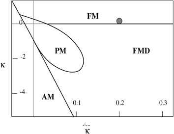
FIG. 3.: Schematic quenched phase diagram.

For calculating the fermion propagators, as in [8] we have chosen the point $\kappa=0.05$, $\tilde{\kappa}=0.2$ (gray blob in Fig.3). Although this point is far away from $\tilde{\kappa}=\infty$, around which we did our perturbation theory in the previous section, the important issue here is to choose a point near the FM-FMD transition and away from the FM-PM transition. The results below show that for the fermion propagators there is excellent agreement between numerical results obtained at $\kappa=0.05$, $\tilde{\kappa}=0.2$ and perturbation theory.

Numerically on $4^{3}16$ and $6^{3}16$ lattices with $L_{s}=22$ and $m_{0}=0.5$ we look for chiral modes at the domain wall ($s=0$), the anti-domain wall ($s=11$), and at the waveguide boundaries ($s=5,6$ and $s=16,17$). Error bars in all the figures are smaller than the symbols.

Fig.4 shows the $RR$ propagator $|S_{RR}|$ and the $LL$ propagator $|S_{LL}|$ at the domain and anti-domain wall as a function of a component of momentum $p_{4}$ for both $\vec{p}=(0,0,0)$ (physical mode) and $(0,0,\pi)$ (first doubler mode) at $y=1$. From the figures, it is clear that the doubler does not exist, only the physical $RR$ ($LL$) propagator seems to have a pole at $p=(0,0,0,0)$ at the anti-domain (domain) wall. In all the figures, NS, PT and FF respectively indicate data from numerical simulation, from perturbation theory and from free fermion propagator by direct inversion of the free fermion matrix.

FIG. 4.: Chiral propagators at domain wall $s=0$ and at anti-domain wall $s=11$ ($L_{s}=22$; a.p.b.c. in $L_{4}$, $y=1.0$).

FIG. 5.: $RR$ propagator at waveguide boundary $s=5$ and $LL$ propagator at waveguide boundary $s=6$ ($L_{s}=22$; a.p.b.c. in $L_{4}$, $y=1.0$).

For Fig.4, PT also means zeroth order perturbation theory, i.e., numerical solution of propagator following eq.(39) (as noted before in subsubsection III B 2 the self-energy contributions to the $LL$ and $RR$ propagators are nonzero only at the waveguide boundaries, the propagators in Fig.4 do not get any 1-loop correction). We have PT results also for $6^{3}\times 16$ lattice but have chosen not to show them because they fall right on top of the numerical data. Instead PT results are shown for $8^{3}\times 20$ lattice for which the $p_{4}$ points are distinct. The dotted line in all figures refer to the propagator from PT using a $256^{3}\times 1024$ lattice. The curves stay the same irrespective of methods or lattice size. Based on the above, we can conclude that there are only free RH fermions at the anti-domain wall, and at the domain wall there are only free LH fermions.

Fig.5 show no evidence of a chiral mode at the waveguide boundaries $s=5$ and 6 and excellent agreement with 1-loop perturbation theory. Here too doublers do not exist. Actually the agreement with the FF method (direct inversion of the free domain wall fermion matrix on a given finite lattice) is also excellent, because the 1-loop corrections are almost insignificant. For clarity, in Fig.5 we have not shown the $LL$ propagator on $s=5$ and the $RR$ propagator at $s=6$, but conclusions are the same.

Similar investigation at the other waveguide boundary $s=16,17$ also does not show any chiral modes. Previous investigations of the domain wall waveguide model without gauge fixing [12] have shown that the waveguide boundaries are the most likely places to have the unwanted mirror modes. This is why we have mostly concentrated in showing that there are no mirror chiral modes at these boundaries, although we have looked for chiral modes everywhere along the flavor dimension. In fact, we do not see any evidence of a chiral mode anywhere other than at the domain wall and the anti-domain wall.

V Discussion

We have followed the gauge fixing proposal of Shamir and Golterman and applied it to domain wall fermions for a $U(1)$ $L\chi GT$. By switching off the transverse gauge dof, we arrive at the so-called reduced model. We have determined the quenched phase diagram of the model and confirmed that there is a continuous phase transition from a broken symmetry ferromagnetic (FM) phase to a broken symmetry rotationally noninvariant ferromagnetic directional (FMD) phase with the properties that at this transition the longitudinal gauge dof, i.e., the $\varphi$ fields get decoupled. We have come to this conclusion by performing a WCPT for the fermion propagators and comparing them to nonperturbative numerical simulations.

Let us now contrast this with the previous attempt [12] of lattice regularizing a chiral gauge theory with domain wall fermions. No gauge fixing was done and in the reduced model, a combination of analytic and numerical methods showed that mirror chiral modes were dynamically generated in the theory.

As in the Smit-Swift model [2], the mirror chiral modes are a reflection of the undesired presence of the longitudinal gauge dof in the continuum limit. Without gauge fixing, these radially frozen group-valued scalar $\varphi$ fields are generally nonperturbative or rough for any value of the transverse gauge coupling, even in the reduced model limit. If the continuum limit is taken at the FM to a symmetric paramagnetic (PM) phase transition, the $\varphi$ fields survive with radial modes and physical effects of them coupling with the rest of the theory become manifest in the form of mirror chiral modes etc..

In the gauge fixing approach of Shamir and Golterman, care has been exercised so that the gauge fixing term is not just a naive lattice transcription of the continuum gauge fixing condition. There are appropriate additions of irrelevant terms in the covariant gauge fixing term so that a unique perturbative vacuum exists. With this gauge fixing in the reduced model limit the $\varphi$ fields become smooth and can be perturbatively expanded as $1+{\cal O}(1/\sqrt{\tilde{\kappa}})+\cdots$ around $\tilde{\kappa}=\infty$. We have found in our investigation that as long as $\tilde{\kappa}$ is taken sufficiently large so that a continuum limit exists from the FM phase to the FMD phase (not the PM phase), the model is as good as at the perturbative limit $\tilde{\kappa}=\infty$. This seems to hold true in our particular implementation, i.e., the domain wall fermion case, in a strong sense, because the perturbative 1-loop corrections (i.e., the leading nontrivial corrections) to the fermion propagators are found to be negligible (Figs. 4 and 5). In gauge fixing the Smit-Swift model, however, 1-loop corrections to the fermion propagators were small but not negligible [8]. In the present investigation with domain wall fermions, to the accuracy of our calculations, the reduced model spectrum is that of a free domain wall model with absolutely no trace of the $\varphi$ fields.

In our investigation of the reduced model, only a counterterm with coefficient $\kappa$ was sufficient to reach the FM-FMD phase transition by decreasing $\kappa$ from the FM-side. A dimension-three fermion mass counterterm was not needed, because domain wall fermions have the robust property that mixing between the opposite chiral modes at the domain wall and the anti-domain wall is exponentially damped and is negligible for large $L_{s}$.

We have carried out and presented the perturbative results for fermion propagators and mass matrix in reasonable detail, because, although the technique employed is not new, the explicit results are available mostly for only the QCD (wall) implementation rather than the wall-antiwall implementation suitable for a chiral gauge theory. With transverse gauge fields back on (and fermions in an anomaly-free representation), the full gauge-fixed domain wall model of $L\chi GT$ is ready for a perturbative treatment with the same techniques as used in this paper if the transverse gauge coupling is perturbative. The model is also ready for a nonperturbative treatment by numerical simulation for strong transverse gauge coupling.

Our numerical computations have been done in the quenched approximation and they agree for the fermion propagators very well with zeroth order perturbation theory with the 1-loop corrections almost negligible in our case. Effects of fermion loops would enter these calculations at least at the 2-loop level. Inclusion of dynamical fermions in our nonperturbative numerical investigation should not affect our results about the spectrum of the model at all if the relevant part of the phase diagram remains qualitatively the same.

So far the gauge fixing method is applicable only to the abelian theory. Extension to a nonabelian gauge group is nontrivial and is being pursued at the current time [9].

As commented at the end of section II, the reduced gauge fixed domain wall model with $0<y<1$ is interesting because at $y=0$ the model is known to have mirror modes at the waveguide boundaries. This will be taken up in a separate publication [15].

A

In this appendix, we describe the boundary conditions used to flavor-diagonalize eqs.(43) and (44) to obtain the results presented in subsection III C and in III D. The boundary conditions make sure that no information passes through the domain wall and the anti-domain wall. This means that the eigensolutions corresponding to a given source flavor index $s$ belonging to a particular segment $0\leq s\leq L_{s}/2$ or $L_{s}/2\leq s\leq L_{s}$ will be restricted to that particular segment. As already stated before, these are not the actual boundary conditions under which the numerical simulations or the analytic calculation for the $LL/RR$ chiral propagators have been performed, for the flavor diagonalization this enables us to calculate the heavy mode solutions and overlap of the chiral modes explicitly. In appendix B we have schematically described how the calculations would go in case of the actual Kaplan boundary conditions, but to obtain explicit expressions would be a horrendous task.

We consider eq.(43) in the region $0\leq s,t\leq L_{s}/2$. Obviously the index $j$ is also in the same region. Writing eq.(43) at $s=L_{s}/2$ gives (by force using the general expression for $M_{0}^{\dagger}M_{0}$ away from the boundaries of the region),

$$\left[1+\tilde{a}(L_{s}/2)^{2}-\left(\lambda^{(0)}_{j}\right)^{2}\right]\left(\phi^{(0)}_{j}\right)_{L_{s}/2}-\tilde{a}(L_{s}/2)\left(\phi^{(0)}_{j}\right)_{L_{s}/2+1}-\tilde{a}(L_{s}/2-1)\left(\phi^{(0)}_{j}\right)_{L_{s}/2-1}=0.$$ (A1)

Again writing eq.(43) at $s=L_{s}/2$ gives (this time using the expression for $M_{0}^{\dagger}M_{0}$ at the boundary of the region and dropping terms that take the solutions across the anti-domain wall),

$$\left[1+\tilde{a}(L_{s}/2)^{2}-\left(\lambda^{(0)}_{j}\right)^{2}\right]\left(\phi^{(0)}_{j}\right)_{L_{s}/2}-\tilde{a}(L_{s}/2-1)\left(\phi^{(0)}_{j}\right)_{L_{s}/2-1}=0.$$ (A2)

For both the eqs.(A1) and (A2) to be true, the following must be true:

$$\left(\phi^{(0)}_{j}\right)_{L_{s}/2+1}=0,$$ (A3)

which is a boundary condition.

Two equations corresponding to the eqs.(A1, A2), this time at $s=0$, are:

$$\left[1+\tilde{a}(0)^{2}-\left(\lambda^{(0)}_{j}\right)^{2}\right]\left(\phi^{(0)}_{j}\right)_{0}-\tilde{a}(0)\left(\phi^{(0)}_{j}\right)_{1}-\tilde{a}(-1)\left(\phi^{(0)}_{j}\right)_{-1}=0,$$ (A4)

$$\left[\tilde{a}(0)^{2}-\left(\lambda^{(0)}_{j}\right)^{2}\right]\left(\phi^{(0)}_{j}\right)_{0}-\tilde{a}(0)\left(\phi^{(0)}_{j}\right)_{1}=0.$$ (A5)

Hence we get the boundary condition at $s=0$ to be

$$\left(\phi^{(0)}_{j}\right)_{0}-\tilde{a}(L_{s}-1)\left(\phi^{(0)}_{j}\right)_{L_{s}-1}=0.$$ (A6)

For the same eigenequation eq.(43) in the other region $L_{s}/2\leq s,t\leq L_{s}$, we similarly get two more boundary conditions as follows:

$$\left(\phi^{(0)}_{j}\right)_{L_{s}/2}-\tilde{a}(L_{s}/2-1)\left(\phi^{(0)}_{j}\right)_{L_{s}/2-1} = 0,$$ (A7)

$$\left(\phi^{(0)}_{j}\right)_{1} = 0.$$ (A8)

These boundary conditions are similar to those given by Shamir [21], except that we get two sets of them, i.e. (A3), (A6), (A7) and (A8), corresponding to two sectors of $s$. Another couple of sets of boundary conditions are obtained for the eigenequation eq.(44) in the two regions in the same way.

B

Here we schematically show that using the correct boundary conditions (in this case the Kaplan boundary conditions, instead of the special boundary conditions explained in Appendix A) does not qualitatively change our conclusions about fermion mass counterterms.

The use of special boundary boundary conditions in sec. III C meant that the 5-th or flavor dimension was basically divided by the domain and the antidomain wall into two segments which did not communicate to each other. As a result a wave incident on a wall got fully reflected. In general, there will be transmission to the other side of the wall.

The chiral zero modes are the same as before (except for a tiny change in the normalization) except that they are now allowed to decay all the way around the $s$-space.

Let us assume then the following trial eigenfunctions $\phi^{\pm}$ and $\Phi^{\pm}$ for the heavy modes:

$$(\phi^{\pm^{(0)}}_{j})_{s} = A_{\pm j}\exp(-i\beta_{\pm j}s)+B_{\pm j}\exp(i\beta_{\pm j}s)$$ (B1)

$$(\Phi^{\pm^{(0)}}_{j})_{s} = C_{\pm j}\exp(-i\beta_{\pm j}s)+D_{\pm j}\exp(i\beta_{\pm j}s).$$ (B2)

The subscripts $\pm$ go with the regions in $s$-space with corresponding signs of $m(s)$ in eq.(5). The wavevectors $\beta$ are obtained by trying these trial solutions in the eigenvalue eqs. (43), (44) and are given as:

$$2\tilde{a}(s)\cos\beta_{\pm j}=1+\tilde{a}(s)^{2}-\lambda_{j}^{2}$$ (B3)

We proceed essentially the same way as in the case with the free propagators except for the fact that here we do not have the inhomogeneous part of the solutions. The boundary conditions used to determine $A_{\pm j},\;B_{\pm j},\;C_{\pm j},\;D_{\pm j}$ are (omitting the subscript $j$ and also the tree level indicating superscript $(0)$ for convenience):

$$\tilde{a}_{0}\phi^{+}_{L_{s}}-\tilde{a}_{-}\phi^{-}_{0} = 0$$ (B4)

$$\tilde{a}_{0}\phi^{-}_{L_{s}/2}-\tilde{a}_{+}\phi^{+}_{L_{s}/2} = 0$$ (B5)

$$(1+\tilde{a}_{0}^{2}-\lambda^{2})\phi^{+}_{L_{s}}-\tilde{a}_{0}\phi^{-}_{1}-\tilde{a}_{+}\phi^{+}_{L_{s}-1} = 0$$ (B6)

$$(1+\tilde{a}_{0}^{2}-\lambda^{2})\phi^{-}_{L_{s}/2}-\tilde{a}_{0}\phi^{+}_{L_{s}/2+1}-\tilde{a}_{-}\phi^{-}_{L_{s}/2-1} = 0$$ (B7)

$$\tilde{a}_{0}\Phi^{-}_{0}-\tilde{a}_{+}\Phi^{+}_{L_{s}} = 0$$ (B9)

$$\tilde{a}_{0}\Phi^{+}_{L_{s}/2}-\tilde{a}_{-}\Phi^{-}_{L_{s}/2} = 0$$ (B10)

$$(1+\tilde{a}_{0}^{2}-\lambda^{2})\Phi^{-}_{0}-\tilde{a}_{0}\Phi^{+}_{L_{s}-1}-\tilde{a}_{-}\Phi^{-}_{1} = 0$$ (B11)

$$(1+\tilde{a}_{0}^{2}-\lambda^{2})\Phi^{+}_{L_{s}/2}-\tilde{a}_{0}\Phi^{-}_{L_{s}/2-1}-\tilde{a}_{+}\Phi^{+}_{L_{s}/2+1} = 0$$ (B12)

where $\tilde{a}_{\pm}=1\pm m_{0}$ and $\tilde{a}_{0}=\tilde{a}_{L_{s}/2}=1$ from eq.(52).

This leads to two sets of linear homogeneous equations for the amplitudes:

$${\bf P}\cdot\Lambda = 0$$ (B13)

$${\bf Q}\cdot\Theta = 0$$ (B14)

where ${\bf P}$ and ${\bf Q}$ are $4\times 4$ matrices and $\Lambda=(A_{-},\;B_{-},\;A_{+},\;B_{+})$ and $\Theta=(C_{-},\;D_{-},\;C_{+},\;D_{+})$. For nontrivial solutions, $\det{\bf P}=0$ and $\det{\bf Q}=0$ leading to (reviving the subscript $j$)

$$\beta_{\pm j}=\frac{2\pi}{L_{s}}j$$ (B15)

Solutions to the eqs.(B14) are of the following general form (dropping the subscripts $j$ again):

$$B_{-} = f_{L}^{(1)}A_{-},\;\;A_{+}=f_{L}^{(2)}A_{-},\;\;B_{+}=f_{L}^{(3)}A_{-}$$ (B16)

$$D_{-} = f_{R}^{(1)}C_{-},\;\;C_{+}=f_{R}^{(2)}C_{-},\;\;D_{+}=f_{R}^{(3)}C_{-}$$ (B17)

where $f_{L,R}^{(1,2,3)}$ are complex numbers with finite magnitude (order 1). $A_{-}$ and $C_{-}$ are determined from normalizations of the respective eigenfunctions and would lead to a ${\cal O}(1/L_{s})$ factor.

At 1-loop with the Kaplan boundary conditions, there is also a contribution to the fermion self-energy for the $LR$ and $RL$ parts coming from a flavor off-diagonal half-circle diagram (we shall call it a global-loop diagram) where the scalar field goes around the flavor space connecting fermions at the waveguide boundaries $I$ and $II$. The global-loop diagram originates from the fact that the $\varphi$ field that couples the fermions at the waveguide boundary $I$ is the same $\varphi$ field coupling the fermions at the waveguide boundary $II$.

FIG. 6.: Global loop contribution to 1-loop $LR$ propagator connecting $WG$ boundaries $I$ and $II$.

Self-energy contribution from the global-loop diagram for the $LR$ propagator is:

$$-\left(\Sigma^{gl}_{LR}(p)\right)_{st} = b^{2}P_{L}\int_{BZ}\frac{d^{4}k}{(2\pi)^{4}}\left[M^{\dagger}(p-k)G_{L}(p-k)\right]_{s_{1}+1,s_{0}}{\cal G}(k)\;\delta_{s,s_{1}}\delta_{t,s_{0}+1}$$ (B18)

$$= b^{2}P_{L}\,{\cal R}\;\delta_{s,s_{1}}\delta_{t,s_{0}+1}$$ (B19)

where ${\cal R}$ is the loop integral in eq.(B18).

Now the calculations for the 1-loop corrected eigenvalue proceeds exactly as in subsection III D, except that it now includes also the contribution from the global-loop diagram:

$$\lambda_{j}=\lambda_{j}^{(0)}+b^{2}\,\left(\overline{{\bf\Sigma}}_{LR}\right)_{jj}$$ (B20)

where, for $|j|\neq 0,\,L_{s}/2$,

$$(\overline{{\bf\Sigma}}_{LR})_{jj} = (\Phi^{\pm^{(0)}}_{j})_{s}\,({\bf\Sigma}_{LR})_{st}\,(\phi^{\pm^{(0)}}_{j})_{t}$$ (B21)

$$= (\Phi^{\pm^{(0)}}_{j})_{s}\,\left(\frac{1}{2}{\cal T}(\delta_{s,s_{0}}\delta_{t,s_{0}+1}+\delta_{s,s_{1}}\delta_{t,s_{1}+1})+{\cal R}\delta_{s,s_{1}}\delta_{t,s_{0}+1}\right)(\phi^{\pm^{(0)}}_{j})_{t}$$ (B22)

$$= \frac{1}{2}{\cal T}\left((\Phi^{-^{(0)}}_{j})_{s_{0}}\,(\phi^{-^{(0)}}_{j})_{s_{0}+1}+(\Phi^{+^{(0)}}_{j})_{s_{1}}\,(\phi^{+^{(0)}}_{j})_{s_{1}+1}\right)+{\cal R}(\Phi^{+^{(0)}}_{j})_{s_{1}}\,(\phi^{-^{(0)}}_{j})_{s_{0}+1},$$ (B23)

and similarly for the chiral zero modes.

Using the expressions for the eigenfunctions at the specific values $s_{0}$, $s_{1}$, $s_{0}+1$ and $s_{1}+1$, we arrive at the 1-loop correction to the eigenvalues:

$$(\delta\lambda)_{j} \sim \frac{b^{2}}{L_{s}}\left({\cal T}{\bf\Omega}_{j}^{(1)}(s_{0},f_{L}^{(1)},f_{R}^{(1)})+{\cal T}{\bf\Omega}_{j}^{(2)}(s_{1},f_{L}^{(2)},f_{L}^{(3)},f_{R}^{(2)},f_{R}^{(3)})+{\cal R}{\bf\Omega}_{j}^{(3)}(s_{0},s_{1},f_{L}^{(1)},f_{L}^{(2)},f_{R}^{(3)})\right),\;|j|\neq 0,\,\frac{L_{s}}{2}$$ (B24)

$$\sim b^{2}{\cal T}\exp[-\tilde{\alpha}(L_{s}/2+1)]+b^{2}{\cal R}\exp[-\tilde{\alpha}(s_{0}+1)-\tilde{\alpha}(L_{s}/2-s_{1})],\;\;\;\;j=0,\,\frac{L_{s}}{2}$$ (B25)

The details of the functions ${\bf\Omega}_{j}^{(n)},\;n=1,2,3$ are not illuminating. Correction to the zero mode eigenvalue clearly shows the exponential damping and for large $L_{s}$ it is negligible.

The 1-loop chiral zero mode wavefunction at the domain wall is,

$$(\phi_{0})_{s} = (\phi^{(0)}_{0})_{s}+b^{2}(\phi^{(1)}_{0})_{j}\,(\phi^{(0)}_{j})_{s}$$ (B26)

$$\sim \exp(-\tilde{\alpha}s)$$ (B28)

$$-\frac{b^{2}}{\lambda^{(0)}_{j}}\left[\frac{1}{2}{\cal T}(\phi^{(0)}_{0})_{s_{0}+1}\,(\Phi^{(0)}_{j})_{s_{0}}(\phi^{(0)}_{j})_{s}+\frac{1}{2}{\cal T}(\phi^{(0)}_{0})_{s_{1}+1}\,(\Phi^{(0)}_{j})_{s_{1}}(\phi^{(0)}_{j})_{s}+{\cal R}(\phi^{(0)}_{0})_{s_{0}+1}\,(\Phi^{(0)}_{j})_{s_{1}}(\phi^{(0)}_{j})_{s}\right]$$

$$\sim \exp(-\tilde{\alpha}s)$$ (B30)

$$-\frac{b^{2}}{2}{\cal T}\exp[-\tilde{\alpha}(s_{0}+1)]\,{\bf\xi}_{1}(s)-\frac{b^{2}}{2}{\cal T}\exp[-\tilde{\alpha}(s_{1}+1)]\,{\bf\xi}_{2}(s)-b^{2}{\cal R}\exp[-\tilde{\alpha}(s_{0}+1)]\,{\bf\xi}_{3}(s),$$

where the well behaved functions ${\bf\xi}_{i},\;i=1,2,3$ contain the information of the heavy mode wavefunctions and need not be written down explicitly (it is to be noted $j\neq 0$ in eq.(B28)). The 1-loop correction to the zero-mode wavefunction is also explicitly damped and for large $L_{s}$ negligible.

The 1-loop correction to zero-mode wavefunction at the anti domain wall is similarly found to be damped. As a result the overlap of the opposite chiral zero modes at the 1-loop level is also exponentially damped.

REFERENCES

- [1]
- [2] W. Bock, A.K. De, J. Smit, Nucl. Phys. B388 (1992) 243; M.F.L. Golterman, D.N. Petcher, J. Smit, Nucl. Phys. B370 (1992) 51
- [3] M. Lüscher, Nucl. Phys. B549 (1999) 295
- [4] Y. Shamir, Phys. Rev. D57 (1998) 132; M.F.L. Golterman, Y. Shamir, Phys. Lett. B399 (1997) 148
- [5] A. Borelli, L. Maiani, G.C. Rossi, R. Sisto, M. Testa, Nucl. Phys. B333 (1990) 335
- [6] H. Neuberger, Phys. Lett. B183 (1987) 337
- [7] W. Bock, M.F.L. Golterman, K.C. Leung, Y. Shamir, hep-lat/9911005
- [8] W. Bock, M.F.L. Golterman, Y. Shamir, Phys. Rev. Lett 80 (1998) 3444
- [9] W.Bock, K.C. Leung, M. Golterman, Y. Shamir, hep-lat/9912025; W.Bock, M. Golterman, M. Ogilvie, Y. Shamir, hep-lat/0004017
- [10] D.B. Kaplan, Phys. Lett. B288 (1992) 342
- [11] D.B. Kaplan, Nucl. Phys.B (Proc. Suppl.) 30 (1993) 597
- [12] M.F.L. Golterman, K. Jansen, D.N. Petcher and J.C. Vink, Phys. Rev. D49 (1994) 1606; M.F.L. Golterman, Y. Shamir, Phys. Rev. D51 (1995) 3026
- [13] W. Bock,M.F.L. Golterman, Y. Shamir, Phys. Rev. D58 (1998) 34501
- [14] S.Basak, A.K.De, Nucl.Phys.B (Proc. Suppl.) 83-84 (2000) 615
- [15] S. Basak, A.K. De, in preparation
- [16] S. Aoki, H. Hirose, Phys. Rev. D54 (1996) 3471
- [17] S. Aoki, Y. Taniguchi, Phys. Rev. D59 (1999) 54510
- [18] T. Blum, A. Soni, M. Wingate, Phys. Rev. D60 (1999) 114507
- [19] S. Aoki, H. Hirose, Phys. Rev. D49 (1994) 2604
- [20] W. Bock, M.F.L. Golterman, Y. Shamir, Phys. Rev. D58 (1998) 54506
- [21] Y. Shamir, Nucl. Phys. B406 (1993) 90