BI-TP 99/35 
November 1999

Goldstone-mode effects and scaling function
for the three-dimensional $O(4)$ model
Jürgen Engels and Tereza Mendes

Fakultät für Physik, Universität Bielefeld, D-33615 Bielefeld, Germany

Abstract

We investigate numerically the three-dimensional $O(4)$ model on $24^{3}$–$120^{3}$ lattices as a function of the magnetic field $H$. We verify explicitly the singularities induced by Goldstone modes in the low-temperature phase of the model, and show that they are also observed close to the critical temperature. Our results are well described by the perturbative form of the model’s magnetic equation of state, with coefficients determined nonperturbatively from our data. The resulting expression is used to generate the magnetization’s scaling function parametrically.

PACS : 64.60.C; 75.10.H; 12.38.Lg

Keywords: Goldstone modes; Scaling function; $O(N)$ models

 
E-mail: engels@physik.uni-bielefeld.de, mendes@physik.uni-bielefeld.de.

1 Introduction

The $O(N)$ spin models (or, more precisely, the $O(N)$-invariant nonlinear $\sigma$-models) are defined by

$$\beta\,{\cal H}\;=\;-J\,\sum_{<i,j>}{\bf S}_{i}\cdot{\bf S}_{j}\;-\;{\bf H}\cdot\,\sum_{i}{\bf S}_{i}\;,$$ (1)

where $i$ and $j$ are nearest-neighbour sites on a $d-$dimensional hypercubic lattice, and ${\bf S}_{i}$ is an $N$-component unit vector at site $i$. The case $N=1$ corresponds to the Ising model. We will consider here only $N>1$. It is convenient to decompose the spin vector ${\bf S}_{i}$ into longitudinal (parallel to the magnetic field ${\bf H}$) and transverse components

$${\bf S}_{i}\;=\;S_{i}^{\parallel}{\bf\hat{H}}+{\bf S}_{i}^{\perp}~{}.$$ (2)

The order parameter of the system, the magnetization $M$, is then the expectation value of the lattice average $S^{\parallel}$ of the longitudinal spin components

$$M\;=\;<\!\frac{1}{V}\sum_{i}S_{i}^{\parallel}>\;=\;<S^{\parallel}>~{}.$$ (3)

Two types of susceptibilities are defined. The longitudinal susceptibility is the usual derivative of the magnetization, whereas the transverse susceptibility corresponds to the fluctuation per component of the lattice average ${\bf S}^{\perp}$ of the transverse spin components

$$\chi_{L}\!\! \!=\! \!\!{\partial M\over\partial H}\;=\;V(<{S^{\parallel}}^{2}>-M^{2})~{},$$ (4)

$$\chi_{T}\!\! \!=\! \!\!V{1\over N-1}<{{\bf S}^{\perp}}^{2}>\;=\;{M\over H}~{}.$$ (5)

These models are of general interest in condensed matter physics, but have applications also in quantum field theory. In particular, the three-dimensional $O(4)$ model is of importance for quantum chromodynamics (QCD) with two degenerate light-quark flavors at finite temperature. If QCD undergoes a second-order chiral transition in the continuum limit, it is believed to belong to the same universality class as the $3d$ $O(4)$ model [1, 2]. QCD lattice data have therefore been compared to the $O(4)$ scaling function, determined numerically in [3]. For staggered fermions this comparison is at present not conclusive [4], but results for Wilson fermions [5] seem to agree quite well with the predictions.

$O(N)$ models in dimension $2<d\leq 4$ are predicted to display singularities on the coexistence line $T<T_{c},H=0$ due to the presence of massless Goldstone modes [6]. In fact, both susceptibilities are predicted to diverge in this region. The magnetic equation of state is nevertheless divergence-free, and compatible with these singularities. The equation of state was calculated up to order $\epsilon^{2}$ in the $\epsilon$-expansion by Brezin et al. [7]. On the basis of this expansion it has been argued [8] that these singularities may be easily observable, since the perturbative coefficient associated with the diverging term is quite large.

A further consequence of the Goldstone singularities is the appearance of strong finite-size effects at all $T<T_{c}$ for $H\to 0$. These effects have been studied using chiral perturbation theory in [9, 10]. Direct numerical evidence of the Goldstone singularities is however lacking, apart from early simulations of the three-dimensional $O(3)$ model on small lattices [11], where indications of the predicted behaviour were found.

The aim of this paper is to verify explicitly the Goldstone singularities, and to investigate their interplay with the critical behaviour and the effect they have on the scaling function. We do this by simulating the three-dimensional $O(4)$ model in the presence of an external magnetic field in the low-temperature phase and close to the critical temperature $T_{c}$. For determining the scaling function, we have also simulated at some high-temperature values. First results of our work have been presented at Lattice’99 [12]. The plan of the paper is as follows. In the next section we review the perturbative predictions for the magnetization and the susceptibilities at low temperatures, as well as the analytic results for the magnetic equation of state, which is equivalent to the magnetization’s scaling function. Our numerical results are discussed in Section 3. The fits and parametrization for the scaling function are given in Section 4. A summary and our conclusions are presented in Section 5.

2 Perturbative Predictions and Critical Behaviour

The continuous symmetry present in the $O(N)$ spin models gives rise to the so-called spin waves: slowly varying (long-wavelength) spin configurations, whose energies may be arbitrarily close to the ground-state energy. In two dimensions these modes are responsible for the absence of spontaneous magnetization, whereas in $d>2$ they are the massless Goldstone modes associated with the spontaneous breaking of the rotational symmetry for temperatures below the critical value $T_{c}$ [13]. For $T<T_{c}$ the system is in a broken phase, i.e. the magnetization $M(T,H)$ attains a finite value $M(T,0)$ at $H=0$. To be definite we assume here $H>0$. As a consequence the transverse susceptibility, which is directly related to the fluctuation of the Goldstone modes, diverges as $H^{-1}$ when $H\to 0$ for all $T<T_{c}$. This can be seen immediately from the identity

$$\chi_{T}\;=\;\frac{M(T,H)}{H}~{}.$$ (6)

This expression is a direct consequence of the $O(N)$ invariance of the zero-field free energy, and can be derived as a Ward identity [7]. It is valid for all values of $T$ and $H$.

A less trivial result [6, 8] is that also the longitudinal susceptibility is diverging on the coexistence curve for $2<d\leq 4$. The leading term in the perturbative expansion for $2<d<4$ is $H^{d/2-2}$. The predicted divergence in $d=3$ is thus

$$\chi_{L}(T<T_{c},H)\;\sim\;H^{-1/2}~{}.$$ (7)

This is equivalent to an $H^{1/2}$-behaviour of the magnetization near the coexistence curve

$$M(T<T_{c},H)\;=\;M(T,0)\,+\,c\,H^{1/2}~{}.$$ (8)

An interesting question is whether the above expressions still describe the behaviour close to the critical region $T\mathrel{\hbox to0.0pt{\lower 3.0pt\hbox{$\mathchar 536\relax$}\hss}\raise 2.0pt\hbox{$\mathchar 316\relax$}}T_{c}$. We recall that the critical behaviour is determined by the singular part of the free energy. Its scaling form in the thermodynamic limit is

$$f_{s}(t,h)\;=\;b^{-d}f_{s}(b^{y_{t}}t,b^{y_{h}}h)~{}.$$ (9)

Here we have neglected possible dependencies on irrelevant scaling fields and exponents. The variables $t$ and $h$ are the conveniently normalized reduced temperature $t=(T-T_{c})/T_{0}$ and magnetic field $h=H/H_{0}$, and $b$ is a free length rescaling factor. The relevant exponents $y_{t,h}$ specify all the other critical exponents

$$y_{t}=1/\nu,\quad y_{h}=1/\nu_{c}~{};$$ (10)

$$\nu_{c}=\nu/\beta\delta,\quad d\nu=\beta(1+\delta),\quad\gamma=\beta(\delta-1)~{}.$$ (11)

Choosing the scale factor $b$ such that $b^{y_{h}}h=1$ and using $M=-\partial f_{s}/\partial H$ one finds the equation

$$M\;=\;h^{1/\delta}f_{G}(t/h^{1/\beta\delta})~{},$$ (12)

where $f_{G}$ is a scaling function. It becomes universal after fixing the normalization constants $H_{0}$ and $T_{0}$. This scaling function was calculated numerically for the $3d$ $O(4)$ model by Toussaint [3] and is used in comparison to QCD lattice data [4, 5].

Alternatively, one may choose $b^{y_{t}}|t|=1$. This leads to the Widom-Griffiths form of the equation of state [14]

$$y\;=\;f(x)\;,$$ (13)

where

$$y\equiv h/M^{\delta},\quad x\equiv t/M^{1/\beta}.$$ (14)

It is usual to normalize $t$ and $h$ such that

$$f(0)=1,\quad f(-1)=0~{}.$$ (15)

The scaling forms in Eqs. (12) and (13) are clearly equivalent. In the following we will work with form (13) and obtain (12) from it parametrically in Section 4.

The equation of state (13) has been derived by Brézin et al. [7] to order $\epsilon^{2}$ in the $\epsilon$-expansion, where $\epsilon=4-d$. Although diverging terms in $\chi_{T}$ appear at intermediate steps of the derivation, they are canceled by diverging $\chi_{L}$ terms, and the resulting expression is divergence-free. This expression has been considered by Wallace and Zia [8] in the limit $x\to-1$, i.e. at $T<T_{c}$ and close to the coexistence curve. In this limit the function is inverted to give $x+1$ as a double expansion in powers of $y$ and $y^{d/2-1}$

$$x+1\;=\;{\widetilde{c}_{1}}y\,+\,{\widetilde{c}_{2}}y^{d/2-1}\,+\,{\widetilde{d}_{1}}y^{2}\,+\,{\widetilde{d}_{2}}y^{d/2}\,+\,{\widetilde{d}_{3}}y^{d-2}\,+\,\ldots\;.$$ (16)

The coefficients ${\widetilde{c}_{1}}$, ${\widetilde{c}_{2}}$ and ${\widetilde{d}_{3}}$ are then obtained from the general expression of [7]. The above form is motivated by the $H$-dependence in the $\epsilon$-expansion of $\chi_{L}$ at low temperatures [8].

In Fig. 1 we show the function $f(x)$ from [7], its low-temperature ($x\to-1$) limit and $f(x)$ from [8], which is obtained from the inverted form of the low-temperature expression, Eq. (16). We see that the low-temperature curve remains close to the general one for a significant portion of the phase diagram, including the critical point at $x=0$, $y=1$ and moving into the high-temperature phase, the region to the right of the critical point. The “inverted” curve and the low-temperature curve that generated it agree quite well. (We remark that the process of inverting produces coefficients that are determined only to order $\epsilon$, while the original low-temperature expression was known to order $\epsilon^{2}$.) As mentioned above, the form (16) is equivalent to the Goldstone-singularity form for $\chi_{L}$ at low temperatures if one identifies the variable $y$ with the field $H$. Nevertheless, the fact that this form may describe the behaviour also at temperatures close to $T_{c}$ and higher is not contradictory, since the variable $y$ can only be identified with $H$ if $M(T,H=0)\neq 0$, which happens only at low temperatures. The form (16) has explicitly nonnegative values of $y$ at $x\approx-1$, while the original perturbative expression produces an unphysical negative $y$ in a

Figure 1: The function $y=f(x)$ (solid line) from [7], its approximation for $x\to-1$ (dashed line) and the inverted form (dotted line) from [8].

very small neighborhood of this point [7]. Possible problems with the form (16) are pointed out in [15, Section 5].

As for the large-$x$ limit (corresponding to $T>T_{c}$ and small $H$), the expected behaviour is given by Griffiths’s analyticity condition [14]

$$f(x)\;=\;\sum_{n=1}^{\infty}a_{n}\,x^{\gamma-2(n-1)\beta}\;.$$ (17)

None of the curves in Fig. 1 approaches this limit, since the low-temperature curves are not valid at large $x$, and the general curve in its original form is known to have problems in this limit [7].

The perturbative equation of state has been used in [2] to produce pictures of the expected behaviour of the $3d$ $O(4)$ model for a large range of temperatures and magnetic fields. The authors have employed an interpolation of the function from [7] with the inverted form from [8] at low temperatures and the Griffiths condition at high temperatures. When compared to Monte Carlo data for the same model in [3], the perturbative scaling function shows qualitative agreement. In Section 4 we propose a fit of our Monte Carlo data to the perturbative form of the equation of state, using (16).

3 Numerical Results

Our simulations are done on lattices with linear extensions $L=24$, 32, 48, 64, 72, 96 and 120 using the cluster algorithm of Ref. [9]. We compute the magnetization $M$ and the susceptibilities $\chi_{L,T}$ at fixed $J=1/T$ (i.e. at fixed $T$) and varying $H$. We note that, due to the presence of a nonzero field, the magnetization is nonzero on finite lattices, contrary to what happens for simulations at $H=0$, where one is led to consider the approximate form $<\!1/V|\sum{\bf S}_{i}|\!>$.

We use the value $J_{c}=0.93590$, obtained in simulations of the zero-field model [16]. In Fig. 2 we show our data for the magnetization for low temperatures up to $T_{c}$ plotted versus $H^{1/2}$. We have simulated at increasingly larger values of $L$ at fixed values of $J$ and $H$ in order to eliminate finite-size effects. The finite-size effects for small $H$ do not disappear as one moves away from $T_{c}$, but rather increase.

In Fig. 3 we plot only the results from our largest lattices. The solid lines are fits to the form (8), and the filled squares at $H>0$ denote the last points included in our fits. It is evident that the predicted behaviour (linear in $H^{1/2}$) holds close to $H=0$ for all temperatures $T<T_{c}$ considered. The Goldstone-mode effects are therefore observable also rather close to $T_{c}$. The straight-line fits coincide with the measured points in a wide range of $H$ for low $T$ (for $J=1.2$ and 1.1 up to $H=0.32$).

Figure 2: The magnetization vs. $H^{1/2}$ in the low-temperature region for fixed $J=1.2$, 1.0, 0.95 and $J_{c}$ and different lattice sizes.

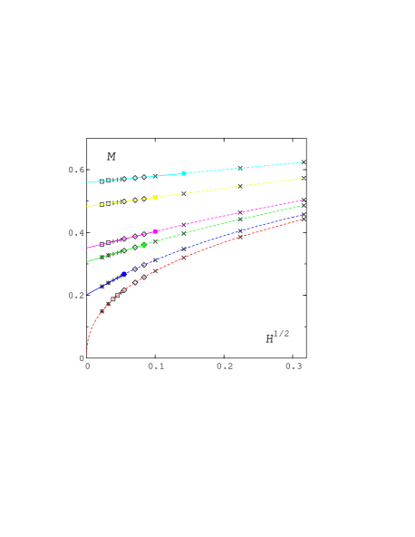
Figure 3: The magnetization as a function of $H^{1/2}$ for fixed $J=1.2$, 1.1, 1.0, 0.98, 0.95 and $J_{c}$, starting with the highest curve. The size $L$ is denoted as in Fig. 2.

$J=1/T$	$M(T,0)$	Slope $c$	$H-$Range	$\chi^{2}/dof$
0.95	0.20202(62)	1.1825(132)	0.001-0.003	0.37
0.98	0.30650(13)	0.6495(26)	0.0005-0.007	0.38
1.00	0.35061(15)	0.5245(20)	0.001-0.01	0.60
1.10	0.48257(29)	0.2940(38)	0.0015-0.01	0.54
1.20	0.55911(13)	0.2033(13)	0.002-0.02	0.92

Table 1: Parameters of the fit of the magnetization to $M(T,0)+cH^{1/2}$.

With increasing $T$ the coincidence region gets smaller and vanishes at $T_{c}$. In Table 1 we have listed the fit parameters. The value $M(T,0)$ obtained from the fits is the infinite-volume value of the magnetization on the coexistence line. In the neighbourhood of $T_{c}$ it should show the usual critical behaviour

$$M(T\mathrel{\hbox to0.0pt{\lower 3.0pt\hbox{$\mathchar 536\relax$}\hss}\raise 2.0pt\hbox{$\mathchar 316\relax$}}T_{c},H=0)\;=\;B(T_{c}-T)^{\beta}\;=\;B(1/J_{c}-1/J)^{\beta}~{}.$$ (18)

Using this simple form, without including any next-to-leading terms, we are able to fit all points of Table 1 with $B=0.9670(5)$ and the exponent $\beta=0.3785(6)$, in agreement with the high-precision zero-field determination in [17].

As the critical point is reached the $H$-dependence of the magnetization should change to satisfy critical scaling. We thus fit the data from the largest lattice sizes at $T_{c}$ to the form

$$M(T_{c},H)\;=\;d_{c}H^{1/\delta}.$$ (19)

As can be seen in Fig. 4a a very good straight-line fit to the largest-$L$ results is possible. The smaller lattices show however definite finite-size effects. We find the exponent $\delta=4.86(1)$, in agreement with [17], and in addition we obtain the critical amplitude $d_{c}=0.715(1)$. In Fig. 4b the magnetization at $T_{c}$ is compared with the finite-size-scaling prediction

$$M(T_{c},H;L)\,=\,L^{-\beta/\nu}\,Q_{M}(H\,L^{\beta\delta/\nu})\;,$$ (20)

using the critical exponents of Ref. [17]. We observe no corrections to scaling, even at higher $H$-values. The scaling function $Q_{M}$ is universal. In order to be consistent with Eq. (19) for large $z\equiv HL^{\beta\delta/\nu}$, i.e. for finite small $H$ and large $L$, it must behave as

$$Q_{M}(z)\;=\;d_{c}z^{1/\delta}.$$ (21)

This offers a second way to determine the critical amplitude $d_{c}$, this time exploiting also the data of the smaller lattices. From a fit in the $z$-range $20-1000$ we find the value $d_{c}=0.713(1)$, which agrees with our first determination.

In Fig. 5 we show an example (at $J=0.98$) of the different behaviours of $\chi_{T}$ and $\chi_{L}$ at low temperatures. As a test we compare the result for $\partial M/\partial H$ (line) from the $M$-fits in Table 1 to the $\chi_{L}$-data. Though there are large finite-size effects for small $L$, the results for the highest $L$-values agree nicely with the expected behaviour. A similar test can be done for $\chi_{T}$ by showing also the result for $M/H$ (line), as obtained from the measurements of the magnetization in Fig. 3. Here as well we find agreement for large $L$.

Figure 4: The magnetization at $T_{c}$. In the left figure (a), $M$ is plotted vs. $H^{1/\delta}$, the line is the fit (19), the solid part shows the range used for the fit. The right plot (b) shows the finite-size-scaling function $Q_{M}$ from Eq. (20).

Figure 5: The susceptibilities below $T_{c}$ at $J=0.98$. On the left $\chi_{L}$ is plotted vs. $H^{-1/2}$. The right plot shows $\chi_{T}$ as a function of $H^{-1}$. The lines are explained in the text.

The $H$-dependencies of the susceptibilities at the critical point are the same. Their amplitudes differ however by a factor $\delta$. Here and in the following we use the values $\delta=4.86$ and $\beta=0.38$ . From Eqs. (4) and (6) and from the magnetization at the critical point, Eq. (19), we derive

$$\chi_{L}\;=\;(d_{c}/\delta)H^{1/\delta-1}~{}\quad{\rm and}\quad\chi_{T}\;=\;d_{c}H^{1/\delta-1}~{}.$$ (22)

In the left part of Fig. 6 we compare $\chi_{L}$ and $\chi_{T}$ at $T_{c}$. The lines in the figure are calculated from Eq. (22) and the fit results of Eq. (19). We see again consistency with the highest-$L$ data. The right part of Fig. 6 shows two examples of $\chi_{L}$ and $\chi_{T}$ for high temperatures. Both susceptibilities converge to one value $\chi(T)$ for $H\to 0$, since no spontaneous symmetry breaking occurs for $T>T_{c}$. At the higher temperature corresponding to $J=0.80$ the two susceptibilities are essentially constant (i.e. the magnetization is linear in $H$) and equal for a large range in $H$. However, at $J=0.90$ (that is closer to $T_{c}$) and finite $H$-values $\chi_{T}$ is larger than $\chi_{L}$.

Figure 6: The susceptibilities at $T_{c}$ (left) vs. $H^{1/\delta-1}$ and above $T_{c}$ (right) vs. $H$ at $J=0.90$ (squares) and $J=0.80$ (circles). The lines are explained in the text.

4 The Scaling Function

The scaling function for the three-dimensional $O(4)$ model was determined from a fit of Monte Carlo data in [3]. Our goal here is to describe our data using the perturbative form of the equation of state as discussed in Section 2, but with nonperturbative coefficients, determined from a fit of the data. The original form of the function $y=f(x)$ from [7] is not suitable for such a fit. We thus consider Eq. (16), which is written as a simple series expansion in $y$. We do not expect this form to describe the data for all $x$ and $y$, yet looking at Fig. 1, we hope to cover a significant portion of the phase diagram for small $x$. The idea is to interpolate this result with a fit to the large-$x$ form (17).

Our fits are shown, together with our data, in Figs. 7 and 8. We have considered data from our largest lattices, for inverse temperatures $0.9\leq J\leq 1.0$ and magnetic fields $H\leq 0.01$. The normalization constants $H_{0}$ and $T_{0}$, obtained from Eq. (15) and our fits in Section 3 are given by

$$H_{0}\;=\;5.08(3)\;,\quad T_{0}\;=\;1.093(2)\;.$$ (23)

We have performed a fit using the three leading terms in (16) for small $y$

$$x_{1}(y)+1\;=\;({\widetilde{c}_{1}}\,+\,{\widetilde{d}_{3}})\,y\,+\,{\widetilde{c}_{2}}\,y^{1/2}\,+\,{\widetilde{d}_{2}}\,y^{3/2}\;.$$ (24)

This form was fitted in the interval $-1<x\mathrel{\hbox to0.0pt{\lower 3.0pt\hbox{$\mathchar 536\relax$}\hss}\raise 2.0pt\hbox{$\mathchar 316\relax$}}1.5$, giving

$${\widetilde{c}_{1}}+{\widetilde{d}_{3}}\,=\,0.345(12)\;,\quad{\widetilde{c}_{2}}\,=\,0.6744(73)\;,\quad{\widetilde{d}_{2}}\,=\,-0.0232(49)\;.$$ (25)

Figure 7: The function $y=f(x)$ from fits to data at small $x$ (red line) and at large $x$ (blue line).

The fit describes all the data at $T<T_{c}$ and also higher, up to $x\approx 5$. This confirms that the expression (16) is valid also away from $x\approx-1$, as observed in Section 2. We note the small value of ${\widetilde{d}_{2}}$. An attempt to include the next power of $y$ leads to a coefficient that is zero within errors. We also see that our data are not sensitive to possible logarithmic corrections to Eq. (16) as proposed in [15]. Our coefficients can be compared to those calculated perturbatively for $N=4$ in Ref. [8]

$${\widetilde{c}_{1}}+{\widetilde{d}_{3}}\,=\,0.528\;,\quad{\widetilde{c}_{2}}\,=\,0.530\;.$$ (26)

For large $x$ we have done a 2-parameter fit of the behaviour (17), in the corresponding form for $x$ in terms of $y$

$$x_{2}(y)\;=\;a\,y^{1/\gamma}\,+\,b\,y^{(1-2\beta)/\gamma}~{}.$$ (27)

Considering data points with $y>50$ (corresponding to $x\mathrel{\hbox to0.0pt{\lower 3.0pt\hbox{$\mathchar 536\relax$}\hss}\raise 2.0pt\hbox{$\mathchar 318\relax$}}15$) we obtain

$$a\,=\,1.084(6)\;,\quad b\,=\,-0.874(25)\;.$$ (28)

Expression (27) is seen to describe the data for $x\mathrel{\hbox to0.0pt{\lower 3.0pt\hbox{$\mathchar 536\relax$}\hss}\raise 2.0pt\hbox{$\mathchar 318\relax$}}2$. We mention that a fit of our data to the leading term in Griffiths’s condition, using $x\geq 50$, yields $\gamma=1.45(1)$, which is in agreement with [17].

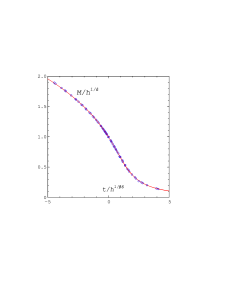
Figure 8: The scaling function $f_{G}=M/h^{1/\delta}$ from Eq. (12). The data are shown together with our fit from Eq. (29).

The small- and large-$x$ curves cover the whole range of values of $x$ remarkably well. In fact, the two curves are approximately superimposed in the interval $2\mathrel{\hbox to0.0pt{\lower 3.0pt\hbox{$\mathchar 536\relax$}\hss}\raise 2.0pt\hbox{$\mathchar 316\relax$}}x\mathrel{\hbox to0.0pt{\lower 3.0pt\hbox{$\mathchar 536\relax$}\hss}\raise 2.0pt\hbox{$\mathchar 316\relax$}}8$. We can therefore interpolate smoothly, for example by taking

$$x(y)\;=\;x_{1}(y)\,\frac{y_{0}^{3}}{y_{0}^{3}+y^{3}}\,+\,x_{2}(y)\,\frac{y^{3}}{y_{0}^{3}+y^{3}}$$ (29)

at $y_{0}=10$, which corresponds to $x\approx 4$. Expression (29) is equivalent to the equation of state (13) and to the scaling function $f_{G}$ in (12). In Fig. 8 we show a plot of $f_{G}$ obtained parametrically from $x(y)$ in (29). The two variables in the plot are simply related to $x$ and $y$ by

$$f_{G}\;=\;M/h^{1/\delta}\;=\;y^{-1/\delta}\;,\quad t/h^{1/\beta\delta}\;=\;x\,y^{-1/\beta\delta}\;.$$ (30)

We see a remarkable agreement of our data points with the form suggested by perturbation theory. With respect to the scaling function in [3] our function is slightly higher for large negative $t/h^{1/\delta\beta}$, due to our more complete elimination of finite-size effects.

5 Summary and Conclusions

We have shown that the Golstone singularities are clearly observable at low temperatures, and also close to $T_{c}$. In fact, we are able to use the observed Goldstone-effect behaviour to extrapolate our data to $H\to 0$ and obtain the zero-field critical exponent $\beta$ in good agreement with [17]. We remark that the same does not happen at high temperatures: we are not able to get the exponent $\gamma$ from extrapolations using the constant behaviour of the longitudinal susceptibility (or the linear behaviour of the magnetization), since this behaviour is masked close to $T_{c}$ for the fields $H$ we have taken into account. At the same $H$’s the $H^{1/2}$ behaviour is clearly present for all the $T<T_{c}$ we consider, showing that the Goldstone effect is dominating the critical one, except at $T_{c}$.

A strong manifestation of the Goldstone behaviour had been conjectured perturbatively [8], based on the size of the coefficient ${\widetilde{c}_{2}}$ in the $\epsilon$-expansion of the equation of state. We have fitted the perturbative form in Section 4, finding a coefficient that is even larger than the perturbative one.

The resulting curve for the equation of state describes all the data beautifully, and can be plotted parametrically for the scaling function.

As a by-product of our work we have determined the critical exponent $\delta=4.86(1)$ by a fit of the magnetization at $T_{c}$ to the critical scaling behaviour as a function of $H$. In addition we checked the finite-size-scaling prediction for $M$. It is remarkable that we observed in both cases no corrections to scaling.

A similar investigation for the $O(2)$ model is currently being done [18].

Acknowledgements

We thank Attilio Cucchieri and Frithjof Karsch for helpful suggestions and comments. Our computer code for the cluster algorithm was based on a zero-field program by Manfred Oevers. This work was supported by the Deutsche Forschungsgemeinschaft under Grant No. Ka 1198/4-1.

References

-
[1]
R. Pisarsky and F. Wilczek,
Phys. Rev. D29 (1984) 338;
F. Wilczek, J. Mod. Phys. A7 (1992) 3911. - [2] K. Rajagopal and F. Wilczek, Nucl. Phys. B399 (1993) 395.
- [3] D. Toussaint, Phys. Rev. D55 (1997) 362.
- [4] C. Bernard et al. (MILC Collaboration), hep-lat/9908008.
- [5] A. Ali Khan et al. (CP-PACS Collaboration), hep-lat/9909075.
- [6] J. Zinn-Justin, Quantum Field Theory and Critical Phenomena, Clarendon Press, Oxford, 1996; R. Anishetty et al., Int. J. Mod. Phys. A14 (1999) 3467.
- [7] E. Brézin, D.J. Wallace and K.G. Wilson, Phys. Rev. B7 (1973) 232.
- [8] D.J. Wallace and R.K.P. Zia, Phys. Rev. B12 (1975) 5340.
- [9] I. Dimitrović, P. Hasenfratz, J. Nager and F. Niedermayer, Nucl. Phys. B350 (1991) 893.
-
[10]
M. Göckeler, K. Jansen and T. Neuhaus,
Phys. Lett. B273 (1991) 450;
I. Dimitrović, J. Nager, K. Jansen and T. Neuhaus, Phys. Lett. B268 (1991) 408. - [11] H. Müller-Krumbhaar, Z. Physik 267 (1974) 261.
- [12] J. Engels and T. Mendes, hep-lat/9909013, to appear in the proceedings of Lattice ’99.
- [13] See e.g. V.G. Vaks, A.I. Larkin and S.A. Pikin, Sov. Phys. JETP 26 (1968) 647.
- [14] R.B. Griffiths, Phys. Rev. 158 (1967) 176.
- [15] A. Pelissetto and E. Vicari, Nucl. Phys. B540 (1999) 639.
- [16] M. Oevers, diploma thesis, Bielefeld University, 1996.
- [17] K. Kanaya and S. Kaya, Phys. Rev. D51 (1995) 2404.
- [18] J. Engels, S. Holtmann, T. Mendes and T. Schulze, in preparation.