FROM BLACK HOLES TO GLUEBALLS:
The $QCD_{3}$ Tensor Glueball at Strong Coupling

Abstract

A strong coupling calculation of glueball masses based on the duality between supergravity and Yang-Mills theory is presented. Earlier work is extended to non-zero spin. Fluctuations in the gravitational metric lead to the $2^{++}$ state on the leading Pomeron trajectory with a mass relation: $m(0^{++})<m(2^{++})<m(1^{-+})$. Contrary to expectation, the mass of our new $0^{++}$ state ($m^{2}=5.4573$) associated with the graviton is smaller than the mass of the ${\tilde{0}}^{++}$ state ($m^{2}=11.588$) from the dilaton, which in fact is exactly degenerate with the tensor $2^{++}$.

1 INTRODUCTION

The Maldacena conjecture [1]  and its further extensions allow us to compute quantities in a strongly coupled gauge theory from its dual gravity description. In particular, Witten [2]  has pointed out if we compactify the 4-dimensional conformal super Yang Mills (SYM) to 3 dimensions using anti-periodic boundary conditions on the fermions, then we break supersymmetry and conformal invariance and obtain a theory that has interesting mass scales. In Refs.[3] and [4], this approach was used to calculate a discrete mass spectrum for ${\tilde{0}}^{++}$ states associated with $Tr[F^{2}]$ at strong coupling by solving the dilaton’s wave equation in the corresponding gravity description. Although the theory at strong coupling is really not pure Yang-Mills, since it has additional fields, some rough agreement was claimed with the pattern of glueball masses. Here we report on the calculation of the discrete modes for the perturbations of the gravitational metric.

2 AdS/CFT DUALITY AT FINITE T

Let us review briefly the proposal for getting a 3-d Yang-Mills theory dual to supergravity. One begins by considering Type IIB supergravity in Euclidean 10-dimensional spacetime with the topology $M_{5}\times S^{5}$. The Maldacena conjecture asserts that IIB superstring theory on $AdS^{5}\times S^{5}$ is dual to the ${\cal N}=4$ SYM conformal field theory on the boundary of the $AdS$ space. The metric of this spacetime is

$$ds^{2}/R^{2}_{ads}=r^{2}(d\tau^{2}+dx^{2}_{1}+dx^{2}_{2}+dx^{2}_{3})+{dr^{2}\over r^{2}}+d\Omega^{2}_{5}\;,$$

where the radius of the $AdS$ spacetime is given through $R^{4}_{AdS}=g_{s}N\alpha^{\prime 2}$ ($g_{s}$ is the string coupling and $l_{s}$ is the string length, $l^{2}_{s}=\alpha^{\prime}$). The Euclidean time is $\tau=ix_{0}$. To break conformal invariance, following [2] , we place the system at a nonzero temperature described by a periodic Euclidean time $\tau=\tau+2\pi R_{0}$. The metric correspondingly changes, for small enough $R_{0}$, to the non-extremal black hole metric in $AdS$ space. For large black hole temperatures, the stable phase of the metric corresponds to a black hole with radius large compared to the $AdS$ curvature scale. To see the physics of discrete modes, we may take the limit of going close to the horizon, whereby the metric reduces to that of the black 3-brane. This metric is (we scale out all dimensionful quantities)

$$ds^{2}=fd\tau^{2}+f^{-1}dr^{2}+r^{2}(dx_{1}^{1}+dx_{2}^{2}+dx_{3}^{2})+d\Omega_{5}^{2}\;,$$

with

$$f(r)=r^{2}-{1\over r^{2}}\;.$$

On the gauge theory side, we would have a $N=4$ susy theory corresponding to the $AdS$ spacetime, but with the $S^{1}$ compactification with antiperiodic boundary conditions for the fermions, supersymmetry is broken and massless scalars are expected to acquire quantum corrections. Consequently from the view point of a 3-d theory, the compactification radius acts as an UV cut-off. Before the compactification the 4-d theory was conformal, and was characterized by a dimensionless effective coupling $({g_{YM}^{(4)}})^{2}N\sim g_{s}N$. After the compactification the theory is not conformal, and the radius of the compact circle provides a length scale. Let this radius be $R_{0}$. Then a naive dimensional reduction from 4-d Yang-Mills to 3-d Yang-Mills, would give an effective coupling in the 3-d theory equal to $(g_{YM}^{(3)})^{2}N=({g_{YM}^{(4)}})^{2}N/R_{0}$. The 3-d YM coupling has the units of mass. If the dimensionless coupling $({g_{YM}^{(4)}})^{2}N$ is much less than unity, then the length scale associated to this mass is larger than the radius of compactification, and we may expect the 3-d theory to be a dimensionally reduced version of the 4-d theory.

Unfortunately the dual supergravity description applies at $({g_{YM}^{(4)}})^{2}N>>1$, so that the higher Kaluza-Klein modes of the $S^{1}$ compactification have lower energy than the mass scale set by the 3-d coupling. Thus we do not really have a 3-d gauge theory with a finite number of additional fields. One may nevertheless expect that some general properties of the dimensionally reduced theory might survive the strong coupling limit. Moreover, we expect that the pattern of spin splittings might be a good place to look for similarities. In keeping with earlier work, we ignore the Kaluza-Klein modes of the $S^{1}$ and restrict ourselves to modes that are singlets of the $SO(6)$, since non-singlets under the $S^{1}$ and the $SO(6)$ can have no counterparts in a dimensionally reduced $QCD_{3}$.

3 WAVE EQUATIONS

We wish to consider fluctuations of the metric of the form,

$$g_{\mu\nu}=\bar{g}_{\mu\nu}+h_{\mu\nu}(x)\;,$$

leading to the linear Einstein equation,

$$h_{\mu\nu;\lambda}{}^{\lambda}+h_{\lambda}^{\lambda}{}_{;\mu\nu}-h_{\mu\lambda;\nu}{}^{\lambda}-h_{\nu\lambda;\mu}{}^{\lambda}-8h_{\mu\nu}=0\;.$$

Our perturbations will have the form

$$h_{\mu\nu}=\epsilon_{\mu\nu}(r)e^{-mx_{3}}$$

where we have chosen to use $x_{3}$ as a Euclidean time direction to define the glueball masses of the 3-d gauge theory. We fix the gauge to $h_{3\mu}=0$.

From the above ansatz and the metric, we see that we have an $SO(2)$ rotational symmetry in the $x_{1}-x_{2}$ space, and we can classify our perturbations with respect spin.

Spin-2: There are two linearly independent perturbations which form the spin-2 representation of $SO(2)$: $h_{12}=h_{21}=q_{T}(r)e^{-mx_{3}},h_{11}=-h_{22}=q_{T}(r)e^{-mx_{3}}\;$ with all  other components  zero. The Einstein equations give,

$$(r^{2}-{1\over r^{2}})q_{T}^{\prime\prime}+(r+{3\over r^{3}})q_{T}^{\prime}+({m^{2}\over r^{2}}-4-{4\over r^{4}})q_{T}=0.$$

Defining $\phi_{T}(r)=q_{T}(r)/r^{2}$, this is the same equation as that satisfied by the dilaton (with constant value on the $S^{5}$).

Spin-1: The Einstein equation for the ansatz, $h_{i\tau}=h_{\tau i}=q_{V}(r)e^{-mx_{3}},{i=1,2}$ gives

$$(r^{2}-{1\over r^{2}})q_{V}^{\prime\prime}+(r-{1\over r^{3}})q_{V}^{\prime}+({m^{2}\over r^{2}}-4+{4\over r^{4}})q_{V}=0\;.$$

Spin-0: Based on the symmetries we choose an ansatz where the nonzero components of the perturbation are

$$h_{11} = h_{22}=q_{1}(r)e^{-mx_{3}}$$

$$h_{\tau\tau} = -2q_{1}(r){f(r)\over r^{2}}e^{-mx_{3}}+q_{2}(r)e^{-mx_{3}}$$

$$h_{rr} = q_{3}(r)e^{-mx_{3}}$$

where $f(r)$ is defined above in the metric. The field equation for $q_{3}\equiv q_{S}(r)$, is

$$p_{2}(r)q^{\prime\prime}_{S}(r)+p_{1}(r)q^{\prime}_{S}(r)+p_{0}(r)q_{S}(r)=0,$$

where $p_{2}(r)=r^{2}(r^{4}-1)^{2}[3(r^{4}-1)+m^{2}r^{2}]$, $p_{1}(r)=r(r^{4}-1)[3(r^{4}-1)(5r^{4}+3)+m^{2}r^{2}(7r^{4}+5)]$ and $p_{0}(r)=9(r^{4}-1)^{3}+2m^{2}r^{2}(3+2r^{4}+3r^{8})+m^{4}r^{4}(r^{4}-1)$.

4 NUMERICAL SOLUTION

To calculate the discrete spectrum for our three equation, one must apply the correct boundary conditions at $r=1$ and $r=\infty$. The result is a Sturm-Liouville problem for the propagation of gravitational fluctuations in a “wave guide”.

Table 1: Glueball Excitation Spectrum.

level	$0^{++}$	$1^{-+}$	$2^{++}$
n= 0	5.4573	18.676	11.588
n= 1	30.442	47.495	34.527
n= 2	65.123	87.722	68.975
n= 3	111.14	139.42	114.91
n= 4	168.60	203.99	172.33
n= 5	237.53	277.24	241.24
n= 6	317.93	363.38	321.63
n= 7	409.82	461.00	413.50
n= 8	513.18	570.11	516.86
n= 9	628.01	690.70	631.71

Using this shooting method we have computed the the first 10 states given in Table 1. The spin-2 equation is equivalent to the dilaton equation solved in Refs. [3] and [4], so the excellent agreement with earlier values validates our method. We used a standard Mathematica routine with boundaries taken to be $x=r^{2}-1=\epsilon$ and $1/x=\epsilon$ reducing $\epsilon$ gradually to $\epsilon=10^{-6}$. Note that since all our eigenfunctions must be even in $r$ with nodes spacing in $x=r^{2}-1$ of $O(m^{2})$, the variable $1/x$ is a natural way to measure the distance to the boundary at infinity. For both boundaries, the values of $\epsilon$ was varied to demonstrate that they were near enough to $r=1,$ and $\infty$ so as not to substantially effect the answer.

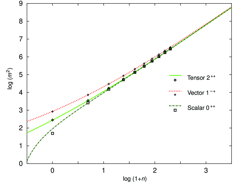
Figure 1: WKB fit to Masses in Table 1

As one sees in the Fig. 1, they match very accurately with the leading order WKB approximation. Simple variational forms also lead to very accurate upper bounds for the ground state ($n=0$) masses.

5 DISCUSSION

Our current exercise needs to be extended to schemes for 4-d QCD such as the finite temperature versions of $AdS^{7}\times S^{4}$. As has been suggested elsewhere, the goal may be to find that background metric that has the phenomenologically best strong coupling limit. This can then provide an improved framework for efforts to find the appropriate formulation of a QCD string and for addressing the question of Pomeron intercept in QCD. In addition, a more thorough analysis of the complete set of spin-parity states for the entire bosonic supergravity multiplet and its extension to 4-d Yang-Mills models is also worthwhile. Results on these computations will be reported in a future publication.

Acknowledgments: We would like to acknowledge useful conversations with R. Jaffe, A. Jevicki, D. Lowe, J. M. Maldacena, H. Ooguri, and others.

References

- [1] J. Maldacena, Adv. Theor. Math. Phys. 2:231, 1998, hep-th/9711200.
- [2] E. Witten, Adv. Theor. Math. Phys.2: 505, 1998, hep-th/9803131.
- [3] C. Csáki, H. Ooguri, Y. Oz and J. Terning, hep-th/9806021.
- [4] R. De Mello Koch, A. Jevicki, M. Mihailescu and J. Nunes, hep-th/9806125.