Efficiency of the UV-filtered Multiboson algorithm

Abstract

We study the efficiency of an improved Multiboson algorithm with two flavours of Wilson fermions in a realistic physical situation ($\beta=5.60$, $\kappa=0.156$ on a $16^{3}\times 24$ lattice). The performance of this exact algorithm is compared with that of a state-of-the-art HMC algorithm: a considerable improvement is obtained for the plaquette auto-correlation time, while the two algorithms appear similarly efficient at decorrelating the topological charge.

I Introduction

The Monte-Carlo simulation of lattice QCD, including the effects of dynamical quark loops, is a particularly difficult and challenging problem, as it involves the computation of the fermion matrix determinant, which appears, after integration over the anti-commuting fermion fields, in the QCD partition function

$${\mathcal{Z}}=\int\prod_{x,\mu}dU_{x,\mu}~{}e^{-S_{g}[U]}~{}\prod_{i=1}^{N_{f}}\det(\mbox{$D$\kern-6.49994pt\hbox{/}\hskip 2.5pt}[U]+m_{i})\quad.$$ (1)

The fermion determinant leads to non-local interactions among the gauge links $U_{x,\mu}$, so that the cost for updating all links naively grows at least as ${\mathcal{O}}(V^{2})$, where $V$ is the lattice volume.

The standard approach to this problem is given by the Hybrid Monte Carlo (HMC) method. The computation of the determinant is achieved stochastically by the introduction of an auxiliary bosonic pseudo-fermion field $\phi$. For the case of two degenerate flavours one may write

$$|\det(\mbox{$D$\kern-6.49994pt\hbox{/}\hskip 2.5pt}+m)|^{2}=\int[d\phi^{\dagger}][d\phi]~{}e^{-|(\not\kern-0.20999ptD+m)^{-1}\phi|^{2}}\quad.$$ (2)

One still has to deal with a non-local action involving $(\mbox{$D$\kern-6.49994pt\hbox{/}\hskip 2.5pt}+m)^{-1}$, but now, using Molecular Dynamics, a global updating of $U$ can be performed.

An alternative approach, which allows the use of local algorithms, is the so-called Multiboson method, originally proposed by Lüscher [1]. If a polynomial $P_{n}(x)=c_{n}\prod_{k=1}^{n}(x-z_{k})$ can be found which approximates $1/x$ over the whole spectrum of $(\mbox{$D$\kern-6.49994pt\hbox{/}\hskip 2.5pt}+m)$, then $P_{n}(\mbox{$D$\kern-6.49994pt\hbox{/}\hskip 2.5pt}+m)\approx(\mbox{$D$\kern-6.49994pt\hbox{/}\hskip 2.5pt}+m)^{-1}$. Using a relation similar to Eq. (2) one can then write

$$|\det(\mbox{$D$\kern-6.49994pt\hbox{/}\hskip 2.5pt}+m)|^{2}\approx|{\det}^{-1}P_{n}(\mbox{$D$\kern-6.49994pt\hbox{/}\hskip 2.5pt}+m)|^{2}$$ (3)

$$~{}~{}~{}~{}~{}~{}~{}~{}~{}~{}~{}=c_{n}^{-V}\int\prod_{k}[d\phi_{k}^{\dagger}][d\phi_{k}]~{}e^{-\sum_{k}|(\not\kern-0.20999ptD+m-z_{k})\phi_{k}|^{2}}\quad.$$ (4)

In this way the original QCD partition function is approximated by a functional integration over the gauge links $U$ and $n$ bosonic fields $\phi_{k}$, where the integration measure is given in terms of a local action

$$S=S_{g}+\sum_{k=1}^{n}|(\mbox{$D$\kern-6.49994pt\hbox{/}\hskip 2.5pt}+m-z_{k})\phi_{k}|^{2}\quad,$$ (5)

so that standard powerful local algorithms (heatbath, overrelaxation) can be used. The systematic error deriving from this approximation can be corrected either during the simulation, with a global accept-reject step, or by a reweighting procedure on physical observables.

An important question to the lattice scientific community is which of the two approaches (HMC or MB) is more efficient for simulating QCD with dynamical fermions. No definitive answer is yet available. On general grounds, the MB method has the advantage of being still relatively new, so that prospects for improvement are much greater.

The MB approach allows two different strategies for improvement. The first is the choice of the approximating polynomial. As the number $n$ of bosonic fields increases, the work per updating step grows as $n$. Moreover, the autocorrelation time for physical observables also grows approximately as $n$. It is therefore essential to choose a polynomial of the lowest possible degree while preserving sufficient accuracy in the approximation, i.e. sufficient acceptance in the Metropolis step. The second is the choice of the update algorithm. Since we are dealing with a local action, a number of possible efficient local algorithms are available. Moreover a global updating of the bosonic field variables can be simply implemented, since their distribution is gaussian. The coupled dynamics of the system (gauge links + boson fields) is highly non trivial, so that the optimal mixture of update algorithms is essentially determined by numerical experiment [2]. As we will see, a good choice can make a substantial difference.

The aim of the present work is to test the efficiency of an improved version of the MB algorithm in a physical situation and to directly compare its performance with a “state of the art” HMC algorithm, namely the one used by the SESAM collaboration [3]. Clearly, the efficiency of an algorithm is different depending on the physical observable one is monitoring (i.e., one obtains different integrated autocorrelation times for different observables). In the present work we are studying the plaquette and the topological charge. These two observables are representative of the smallest- (UV) and largest- (IR) scale features of the gauge field. Therefore, their Monte Carlo dynamics provide a succinct description of the efficiency of a simulation at decorrelating all intermediate scales. The study of the topological charge dynamics is of particular importance: because of the associated zero-mode crossing, it is expected theoretically, and has been shown in practice [4], that HMC algorithms near the chiral limit can be particularly inefficient at decorrelating topology, so that even using a very long simulation time on supercomputers, one is not able to properly sample the topological modes of the theory and ensure ergodicity. The efficiency of the MultiBoson method in this respect has not been studied yet.

We have used the exact, non-hermitian version of the MB algorithm [5] with two flavours of Wilson fermions. In order to reduce the number of bosonic fields we have used the method proposed in [6]: after a preconditioning of the Dirac matrix, which rewrites the effect of the UV fermionic degrees of freedom as a simple modification of the pure gauge action (UV-filtering), an optimized polynomial is constructed numerically by adapting it, via quadratic minimization, to a typical configuration of the physical ensemble.

The dynamics of the algorithm have then been improved by choosing a proper mixture of local overrelaxation of the boson and gauge fields and of global heatbath on the boson fields. The introduction of the global heatbath step (whose computational cost is strongly reduced by using a Quasi-Heatbath with approximate inversion [7]) turns out to be essential in order to improve the dynamics of the algorithm at small quark mass [8].

In Section II we present more details about the algorithm used. In Section III the numerical results of our simulations are shown. In Section IV we give our conclusions.

II Description of the algorithm

A Statics

We have used the exact, non-hermitian version of the MB algorithm [5], which includes a noisy Metropolis test to correct for the polynomial approximation to the fermionic determinant [9].

As the degree $n$ of the approximating polynomial is increased, the work per independent configuration grows as $n^{2}$ [5]: it is therefore crucial to keep $n$ as low as possible while maintaining a good approximation, i.e. a good acceptance for the Metropolis test.

In order to do that we have followed the procedure of [6]. Inspired by the loop expansion of the fermion determinant,

$${\rm det}({\bf 1}-\kappa M)=e^{{\rm Tr~{}Log}({\bf 1}-\kappa M)}=e^{-\sum_{l}\frac{\kappa^{l}}{l}{\rm Tr}~{}M^{l}},$$ (6)

one rewrites the determinant as

$${\rm det}({\bf 1}-\kappa M)=$$ (7)

$$e^{-\sum_{j}a_{j}{\rm Tr}M^{j}}\times{\rm det}\left(({\bf 1}-\kappa M)~{}~{}e^{+\sum_{j}a_{j}M^{j}}\right)$$ (8)

where the identity ${\rm det}~{}e^{A}=e^{{\rm Tr}~{}A}$ has been used.

The idea behind this is to filter out the UV part of the Dirac spectrum: the term $e^{-\sum_{j}a_{j}{\rm Tr}M^{j}}$, which adds a set of small loops to the gauge action, accounts for the UV modes of the fermion determinant. In this way the zeros of the new polynomial (i.e. the one which approximates the inverse of $({\bf 1}-\kappa M)~{}~{}e^{+\sum_{j}a_{j}M^{j}}\>$) can be concentrated near the small eigenvalues (corresponding to IR modes) and a better approximation can be obtained with less cost.

The number of coefficients $\{a_{j}\}$ as well as their values can be optimized. It is easy to see that for $j\leq 4$ the term $e^{-\sum_{j}a_{j}{\rm Tr}~{}M^{j}}$ can be reabsorbed in a shift of the coupling $\beta$ of the pure gauge Wilson action, $\Delta\beta=192\kappa^{4}a_{4}$, so that no computational overhead is incurred.

For the optimization of the coefficients $\{a_{j}\}$ and of the zeros $\{z_{k}\}$ of the polynomial we have followed the procedure suggested in [6], which we describe here briefly. The parameters have to be chosen so that $\det W\simeq 1$, where $W\equiv\prod_{k}^{n}({\bf 1}-\kappa M-z_{k}{\bf 1})\cdot({\bf 1}-\kappa M)\cdot e^{\sum_{j=0}^{m-1}a_{j}M^{j}}$. A sufficient condition for this is that $W\eta\simeq\eta$ for Gaussian vectors $\eta$. Therefore one takes an equilibrium gauge configuration, fixes the coefficients $a_{j}$ to some initial value, draws one or more Gaussian vectors $\eta$ and finds, by quadratic minimization, the roots $\{z_{k}\}$ which minimize the quantity $e=\parallel W\eta-\eta\parallel^{2}$.

During this procedure also $\partial e/\partial a_{j}$ can be computed, so that one can repeat this optimization using new values for $a_{j}$, and thus minimize also with respect to the $a_{j}$’s by Newton’s method.

In principle one should perform an average over different equilibrium gauge fields. In practice results do not change appreciably with the gauge field, so that one single configuration gives sufficient information.

An interesting byproduct of the optimization is that it is possible to estimate the acceptance for the Metropolis test expected during the actual Monte Carlo simulation. The acceptance probability for $\{U_{old}\}\to\{U_{new}\}$ is

$$min(1,\langle\frac{e^{-|W_{{\rm old}}\>\eta|^{2}+|\eta|^{2}}}{e^{-|W_{{\rm new}}\>\eta|^{2}+|\eta|^{2}}}\rangle_{\eta})$$ (9)

and a good estimate for this is ${\rm erfc}(c\parallel W_{{\rm old}}\>\eta-\eta\parallel)$, with $c\sim O(1)$. This estimate can be directly obtained as a result of the optimization procedure.

B Dynamics

As we will show in the next Section, the UV filtering is very effective in reducing the number of fields by a factor 3 or more. The improvement may be really impressive for heavy quarks, since in this case the small loops account for most of the dynamical effects.

However, as the quark mass decreases, one must include larger loops in the gauge action or increase the number of boson fields. Because the multiplicity of larger Wilson loops increases combinatorically, the best compromise (see next Section) limits the loop expansion to small loops and increases the number of fields, which eventually diverges as $1/m_{q}$ [5]. In this case the dynamics of the system may be highly non trivial and the proper choice of the algorithm, or mixture of algorithms, may become very important.

In particular, for light quark masses it is more likely for one of the zeros of the polynomial to get very close to the Dirac spectrum boundary, and so for the corresponding boson field to become almost massless. The dynamics of those IR boson fields then becomes critical. They represent the bottleneck of the dynamical evolution of the whole system. One has then to search for a good algorithm in order to speed up those slow modes.

Due to the simple form of the bosonic distribution,

$$P(\phi_{k})\propto{\rm exp}\left(-|(D-z_{k})\phi_{k}|^{2}\right),$$ (10)

a global heatbath on the bosonic fields can be simply implemented [8] and turns out to be very effective. The new field $\phi_{k}^{\rm NEW}$ is obtained by applying $(D-z_{k})^{-1}$ to a Gaussian vector $\eta$

$$\phi_{k}^{\rm NEW}=(D-z_{k})^{-1}\eta.$$ (11)

In this way $\phi_{k}^{\rm NEW}$ is completely uncorrelated from the old bosonic field.

In practice, since an accurate exact inversion of $(D-z_{k})$ is needed, the global heatbath may become prohibitively expensive, especially for those fields where $z_{k}$ is very close to the edge of the Dirac spectrum, so that $(D-z_{k})$ is almost singular.

In order to cure this problem we have adopted, instead of the usual heatbath with exact inversion, a quasi-heatbath consisting of an approximate inversion plus a Metropolis accept-reject step as proposed in [7].

The idea is not to perform an exact inversion of $(D-z_{k})$, but to stop the inversion algorithm (BiCG in our case) early by loosening the convergence criterion. In order to preserve detailed balance, the system one solves approximately is

$$(D-z_{k})x=b,$$ (12)

with right-hand side $b=(D-z_{k})\phi_{k}^{\rm OLD}+\eta$. The residual is $r=b-(D-z_{k})x$. A candidate bosonic field is then formed as

$$\phi_{k}^{\rm NEW}=x-\phi_{k}^{\rm OLD}.$$ (13)

It is accepted with probability

$$min\left(1,{\rm exp}(2Re(r^{\dagger}.(D-z_{k})(\phi_{k}^{\rm NEW}-\phi_{k}^{\rm OLD})\right)$$ (14)

It is easily proven that in this way the bosonic field is sampled with the correct distribution, for any convergence criterion of the solver. Using this simple trick it is possible to strongly reduce the number of iterations of the inversion algorithm (by a factor 3 or so) while maintaining an acceptance for $\phi_{k}^{\rm NEW}$ close to 1 [7]. The use of even-odd preconditioning further reduces the computational demand.

This global update of the bosonic fields has then to be combined with local update algorithms. We have chosen local overrelaxation for both gauge and bosonic fields.

A good tuning of the relative frequencies of the three different algorithms in the mixture is essential. With the global heatbath some new uncorrelated information is brought into the statistical system via the boson fields, which of course needs some time to propagate to the gauge fields too. While a stochastic choice (with proper weights) among the three algorithms might seem preferable, we have observed that the use of a deterministic sequence of algorithms in the trajectory between two successive Metropolis steps is much more effective.

III Numerical results

Three representative systems, increasingly demanding in computer resources, have been studied: medium-heavy quarks in a small lattice, light quarks in a small lattice, and light quarks in a large lattice. In all three cases the efficiency of our algorithm at least matched that of HMC. Our simulations are of length ${\cal O}(10^{3})\tau_{int}(\Box)$, sufficient to extract reasonably accurate (${\cal O}(10\%)$) integrated autocorrelation times $\tau_{int}(\Box)$ for the plaquette.

In all cases we simulate 2 flavours of Wilson fermions, and use the non-hermitian version of the MultiBoson algorithm [5] with even-odd preconditioning and noisy Metropolis correction test. The gauge action is the Wilson plaquette action.

We have implemented UV-filtering up to fourth order (i.e. up to 4-link loops), which generates a shift $\Delta\beta$ in the gauge coupling $\beta$, but causes no overhead.

The details of the three simulations, denoted (A),(B) and (C), are summarized in Table I. Note that the optimized value of the coefficient $a_{4}$, and thus $\Delta\beta$, is much larger than the hopping parameter expansion value ($1/4$). This is because UV-filtering does its best to approximate the infinite series given by the hopping parameter expansion with a series truncated to 4th order: the best truncated series is not the truncation of the infinite one.

When performing the Metropolis test between two trajectories the quantity $W\eta$, where $W\equiv\prod_{k}^{n}({\bf 1}-\kappa M-z_{k}{\bf 1})\cdot({\bf 1}-\kappa M)\cdot e^{\sum_{j=0}^{m-1}a_{j}M^{j}}$, has to be computed, and some care is needed in the evaluation of the exponential $\xi=e^{\sum_{j=0}^{m-1}a_{j}M^{j}}\eta$. Our method is to compute it by Taylor expansion, stopping the series when the contribution of the first neglected order to $\xi$ is less than $10^{-14}$ for each site.

For MB simulations (A) and (B), the order of update of the gauge links was not the usual one. All 8 links attached to a given site $x$, forming a “star” pattern, were updated before proceeding to another set of 8 links. This arrangement allows a re-use of intermediate link-products in the calculation of the gauge force, thereby reducing the overall amount of computation [10]. More importantly, it becomes very simple in this scheme to integrate analytically over the central bosonic fields $\phi_{k}(x)$, which permits a larger-step update of the gauge fields. This provides similar advantages to the combined gauge-boson update of [2], without the overhead.

The HMC simulations used for comparisons incorporate state-of-the-art improvements: even-odd preconditioning ((A), (B) and (C)); incomplete convergence of the solver during the MD trajectory ((A) and (B)) or time-extrapolation of the initial guess ((C)); BiCG$\gamma_{5}$ ((A) and (B)) or BiCGStab ((C)) solver; multi-stepsize integration, following [11], in ((A) and (B)). Simulation (C) is a SESAM-collaboration production run [3]. It does not incorporate, however, SSOR preconditioning which they use with advantage in more recent projects where it reduces the work per independent configuration by a factor of about two [12].

TABLE I.: Summary of the parameters of our 3 simulations. The optimized coefficients $a_{2}$ and $a_{4}$ and $\Delta\beta$ have been rounded off to 3 decimals. Integrated autocorrelation times are measured in applications of the Wilson Dirac matrix to a vector.

Simulation	A	B	C
Volume	$8^{4}$	$8^{4}$	$16^{3}\times 24$
$\beta,\kappa$	$5.3,0.158$	$5.3,0.165$	$5.6,0.156$
$n_{bosons}$	7	16	24
$a_{2}$	4.411	6.066	4.077
$a_{4}$	1.389	4.423	8.789
$\Delta\beta=192\kappa^{4}a_{4}$	0.166	0.629	0.999
$\tau_{int}(\Box)(MB)$	$\sim 3500$	$\sim 64000$	$\sim 27500$
$\tau_{int}(\Box)(HMC)$	$\sim 14000$	$\sim 72000$	$\sim 85000^{\dagger}$

$\dagger$ Obtained from the SESAM-collaboration data on a $16^{3}\times 32$ lattice [3].

A Medium-heavy quarks, small lattice

The parameters of the simulation are indicated in Table I, column (A). Seven auxiliary fields only were required after UV-filtering (note that there is no need for the number of fields to be even). Fig.1 shows the location of the associated complex zeros of the approximating polynomial, together with the boundary of the Dirac spectrum estimated by diagonalizing the tridiagonal matrix given by the BiCG$\gamma_{5}$ solver. Only one zero is devoted to controlling the UV part of the Dirac spectrum, while the other 6 control the IR. This is because the shift $\Delta\beta\approx 0.166$ in the gauge coupling accounts for most of the UV fluctuations already. Because none of the auxiliary fields has a small mass, as can be judged from the distance of the zeros to the boundary of the Dirac spectrum Fig.1, local and global updates of these fields are about equally efficient. In both cases, the plaquette decorrelates about 4 times faster than with HMC, as shown in Fig.2. This good result is inherent to the MB approach: for heavy quarks, it reduces to pure gauge local updates, whereas HMC remains an infinitesimal-step algorithm with much slower dynamics [13]. Therefore, the relevant question is: at which quark mass, if any, does the MB approach lose its advantage? This is the reason for our second test.

FIG. 1.: Zeros of the UV-filtered polynomial (circles), and estimated boundary of the Dirac spectrum (crosses), simulation (A).

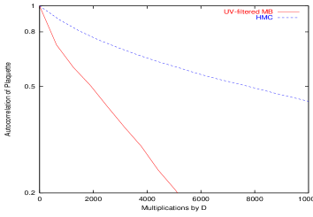
FIG. 2.: Autocorrelation of the plaquette, with the UV-filtered MB algorithm (solid line) and the HMC algorithm (dashed line) at $\beta=5.3$ and $\kappa=0.158$ (simulation A).

B Light quarks, small lattice

The parameters of the simulation are indicated in Table I, column (B). $\kappa_{c}$ is approximately 0.1686(3) [14], so we are simulating light quarks. As appears clearly in Fig.3, several of the IR zeros are now closer to the Dirac spectrum boundary. Consequently, the global Quasi-Heatbath provides a large improvement over local updates, by a factor 5 or more. The number of boson fields, $n=16$, is very much smaller than the number of solver iterations per HMC step ($\sim 53$). The 2 algorithms appear about equally efficient (see Fig.4). Since the work per independent configuration grows more slowly with the volume for MB than HMC ($V(Log(V))^{2}$ vs $V^{5/4}$ [5]), this bodes well for realistic simulations in large volumes.

FIG. 3.: Zeros of the UV-filtered polynomial (circles), and estimated boundary of the Dirac spectrum (crosses), simulation (B).

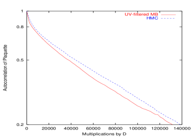
FIG. 4.: Autocorrelation of the plaquette, with the UV-filtered MB algorithm (solid line) and the HMC algorithm (dashed line) at $\beta=5.3$ and $\kappa=0.165$ (simulation B).

C Light quarks, large lattice

The parameters of the simulation are indicated in Table I, column (C). This large-scale simulation has been performed on the APE/TOWER machine in Pisa.

The number of boson fields, $n=24$, is again very much smaller than the number of BiCG iterations per MD step ($\sim 91$). Note that without UV-filtering, these 2 numbers become comparable: we needed $n=80$ fields in this case, with the zeros of the polynomial evenly spaced on the unit circle centered at $(1,0)$, to reach similar acceptance ($\sim 74\%$).

Regarding the mixture of algorithms, we have found that a good compromise is to perform a global heatbath per bosonic field or each symmetrized trajectory composed of 12 couples of local over-relaxation sweeps for the bosonic and gauge fields. This choice may be subject to further optimization.

Of the optimized roots of the UV-filtered polynomial, shown in Fig.5, 16 are devoted to IR modes and 8 to UV modes of the Dirac operator.

FIG. 5.: Zeros of the UV-filtered polynomial ($n=24$)(circles), of the non-UV-filtered polynomial ($n=80$)(+), and estimated boundary of the Dirac spectrum (crosses), simulation (C).

To illustrate the benefits of UV-filtering and of the bosonic quasi-heatbath, we show in Fig.6 the evolution of the plaquette, first without UV-filtering ($n=80$ bosonic fields), then with UV-filtering ($n=24$) but without quasi-heatbath, and finally with both features. The improvement is clearly visible in each case. The autocorrelation of the plaquette is compared in Fig.7 with that obtained by the SESAM collaboration using HMC [3]. Our MB approach is more efficient by a factor $\sim 3$.

In Fig. 8 we compare the topological charge histories obtained from our simulation and from a sample of SESAM configurations [15]. In both cases the same cooling method was used. Neither simulation is long enough to extract a reliable autocorrelation time for this observable. Attempts at doing so yield roughly equivalent results for both algorithms, as the figure already indicates. Therefore, even for this global observable, our MB method seems not worse than HMC.

FIG. 6.: Monte Carlo history of the plaquette, with the non-hermitian MB algorithm (I), then with UV-filtering (II), finally with UV-filtering and bosonic quasi-heatbath (III) (simulation C).

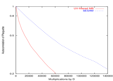
FIG. 7.: Autocorrelation of the plaquette, with the UV-filtered MB algorithm (solid line) and the SESAM HMC algorithm (dashed line) at $\beta=5.6$ and $\kappa=0.156$ (simulation C).

FIG. 8.: Comparison of topological charge histories obtained with HMC and UV-filtered MB algorithm at $\beta=5.6$ and $\kappa=0.156$. The common scale has been set in terms of equivalent $D\times v$ multiplications.

We considered extending the UV-filtering to order 6. This would allow a further reduction of the number of bosonic fields, at the expense of including in the action 6-link loops coming from $Tr(M^{6})$. The optimization of the UV-filtered polynomial was performed under these premises. It indicated that the same accuracy obtained with $n=24$ and 4th-order UV-filtering could be obtained with $n\approx 20$ and 6th-order UV-filtering. This relatively small reduction in $n$ did not justify the overhead of including 6-link loops in the update.

IV Conclusions

We have presented numerical evidence that the exact, non-hermitian MB algorithm is a superior alternative to the traditional HMC: it decorrelates the plaquette more efficiently, and the topological charge equivalently well. The key ingredients to achieve this efficiency are UV-filtering and global quasi-heatbath of the boson fields. The former absorbs the UV modes of the Dirac operator in the gauge action, and thereby reduces the required number of bosonic fields by a factor 3 or more, thus removing the memory bottleneck of the non-filtered MB. The latter greatly accelerates, at low computer cost, the dynamics of the IR, low-mass boson fields. The same scheme can be implemented without changes to simulations with staggered fermions. Similar efficiency gains are expected. At the same time, the MB polynomial can be tailored to approximate any number of staggered flavours, for instance $N_{f}=2$. With a correction step as used for $N_{f}=1$ Wilson-quark simulations [16], this will allow for exact, efficient simulation of two staggered flavours, which are inaccessible to HMC.

We thank Adriano Di Giacomo, Klaus Schilling and Thomas Lippert for interesting discussions, and the whole SESAM collaboration for sharing with us their numerical results. Ph. de F. thanks Greg Kilcup for access to NERSC computers. M. D’E. thanks Lele Tripiccione for his valuable help in using the 512 node APE–QUADRICS in Pisa. Ph. de F. and M. D’E. thank the Aspen Center for Physics where part of this paper was written.

REFERENCES

- [1] M. Lüscher, Nucl. Phys. B418 (1994) 637.
- [2] B. Jegerlehner, Nucl. Phy. B465 (1996) 487.
- [3] SESAM+TL collaboration, Th. Lippert et al., Nucl. Phys. (Proc. Suppl.) B 63 (1998) 946.
- [4] B. Allés, G. Boyd, M. D’Elia, A. Di Giacomo, E. Vicari, Phys. Lett. B 389 (1996) 107.
- [5] A. Borrelli, Ph. de Forcrand and A. Galli, Nucl. Phys. B477 (1996) 809.
- [6] Ph. de Forcrand, hep-lat/9809145, to appear in Nucl. Phys. (Proc. Suppl.).
- [7] Ph. de Forcrand, Phys. Rev. E 59 (1999) 3698.
- [8] A. Boriçi, hep-lat/9602018, unpublished.
- [9] A. Boriçi and Ph. de Forcrand, Nucl. Phys. B 454 (1995) 645.
- [10] Ph. de Forcrand, D. Lellouch and C. Roiesnel, J. Comp. Phys. 59 (1985) 324.
- [11] J. Sexton and D. Weingarten, Nucl. Phys. B 380 (1992) 665.
- [12] SESAM collaboration, S. Fischer et al., Comp. Phys. Comm. 98 (1996) 20; W. Bietenholz et al., hep-lat/9807013, to appear in Comp. Phys. Comm.
- [13] R. Gupta et al., Mod. Phys. Lett. A3 (1988) 1367.
- [14] R. Gupta et al., Phys. Rev. D 40 (1989) 2072.
- [15] B. Allés et al., Phys. Rev. D58 (1998) 071503
- [16] C. Alexandrou et al., hep-lat/9811028, Phys. Rev. D (in press).