hep-lat/9906030 UTHEP-405 Scaling property of domain-wall QCD in perturbation theory

Junichi Noaki and Yusuke Taniguchi Institute of Physics, University of Tsukuba, Tsukuba, Ibaraki 305-8571, Japan
Abstract

We estimate the lattice artifacts in loop correction perturbatively for domain-wall QCD with infinite number of extra flavors. We find that there appear no ${\cal O}(a)$ errors in renormalization factors of quark wave function, mass and quark bilinear operators at one and two loop level with off-shell quark momentum. Our proof is based on even or oddness of the quantum correction in terms of the quark external momentum and mass, and it can be extended to any loop level.

pacs:
11.15Ha, 11.30Rd, 12.38Bx, 12.38Gc

I Introduction

Symanzik’s improvement program[1] applied to on-shell quantities[2] attempts to eliminate cut-off dependence order by order by an expansion in powers of the lattice spacing $a$. In order to improve the Wilson quark action to ${\cal O}(a)$ in lattice QCD, this requires adding the ${\cal O}(a)$ “clover” term [3]. Quark operators also have to be modified by ${\cal O}(a)$ counter terms, which generally involve new operators of higher dimension[4, 5, 6]. In perturbation theory, the tree-level value of the clover coefficient and those of the counter terms of quark operators are sufficient to remove terms of ${\cal O}(g^{2}a\log a)$ in on-shell Green’s functions evaluated at one-loop level[4]. However there still remains ${\cal O}(g^{2}a)$ terms and new counter terms are needed to eliminate them [7, 8].

The domain-wall fermion formulation was originally proposed by Kaplan[9] to define lattice chiral gauge theories with the introduction of many heavy regulator fields as an extension of the Wilson fermion. This original idea and the later work about the Chern-Simons currents[10] is further developed by Shamir[11, 12] into a simpler form and is applied to lattice QCD (DWQCD) anticipating superior features over other quark formulations: no need of the fine tuning to realize the chiral limit and no restriction for the number of flavors. Recent simulation results seem to support the former feature non-perturbatively[13, 14, 15, 16]. It is also perturbatively shown that the massless mode at the tree level still remains stable against the quantum correction[22]. In spite of the existence of the Wilson term in the action it does not directly affect the mass term; there is no additive mass correction.

Related to this good chiral property and disappearance of additive mass correction from the Wilson term the DWQCD is expected to have no next leading ${\cal O}(a)$ errors. It was argued in Ref. [14] with an intuitive discussion of good chirality that the leading discretization errors are ${\cal O}(a^{2})$ and there is no ${\cal O}(a)$ errors. They also argue that the scaling behavior of numerical results for $B_{K}$[13] and strange quark mass[14] are consistent with this nature. For the two dimensional Gross-Neveu model it is reported in Ref.[17] that the physical observables do not have ${\cal O}(a)$ errors by a nonperturbative analysis of the effective potential at large $N$ limit.

Although the lattice axial symmetry was discovered[18] for the Dirac operator which satisfy the Ginsparg-Wilson relation[19, 20]

$\displaystyle\left\{D,\gamma_{5}\right\}=aDR\gamma_{5}D$ (I.1)

and it was shown to exist in the effective theory of DWQCD[21], disappearance of ${\cal O}(a)$ term is not necessarily trivial. Because the lattice axial transformation of Lüscher type contains ${\cal O}(a)$ term within the transformation itself,

$\displaystyle\delta\psi=\gamma_{5}(1-aRD)\psi,\quad\delta{\overline{\psi}}={\overline{\psi}}\gamma_{5}$ (I.2)

and the operators with exact chirality is given by using the projection

$\displaystyle{\cal O}_{\Gamma}={\overline{\psi}}\Gamma\left(1-\frac{a}{2}RD\right)\psi.$ (I.3)

This projected operator can be written in terms of the boundary fermion field of the DWQCD ${\cal O}_{\Gamma}={\overline{q}}\Gamma q$[21], where the boundary fields are given by

$\displaystyle q=\left(1-\frac{a}{2}RD\right)\psi,\quad{\overline{q}}={\overline{\psi}}$ (I.4)

and are transformed under the axial transformation (I.2) as

$\displaystyle\delta q=\gamma_{5}q,\quad\delta{\overline{q}}={\overline{q}}\gamma_{5}.$ (I.5)

In the context of the DWQCD, where the exact axial symmetry does not exist because of infinite number of “unphysical” fermion fields, the chirality of the operator is understood by the axial Ward-Takahashi identity given by Furman and Shamir with an appropriately defined axial transformation[12],

$\displaystyle\nabla_{\mu}\left\langle A_{\mu}^{a}(x){\cal O}\right\rangle=2m\left\langle J_{5}^{a}(x){\cal O}\right\rangle+\left\langle J_{5q}^{a}(x){\cal O}\right\rangle+i\left\langle\delta_{A}^{a}{\cal O}\right\rangle,$ (I.6)

where $A_{\mu}^{a}$ is an axial current, $J_{5}^{a}$ is a pseudo scalar density and $J_{5q}^{a}$ is an explicit breaking term. It was shown in Ref. [12] that the exact axial Ward-Takahashi identity is satisfied for boundary quark operators in the infinite flavor limit,

$\displaystyle\nabla_{\mu}\left\langle A_{\mu}^{a}(x){\cal O}(q,{\overline{q}})\right\rangle=2m\left\langle J_{5}^{a}(x){\cal O}(q,{\overline{q}})\right\rangle+i\left\langle\delta_{A}^{a}{\cal O}(q,{\overline{q}})\right\rangle.$ (I.7)

The above operator ${\cal O}_{\Gamma}={\overline{q}}\Gamma q$ transforms in the same way as in the continuum under the transformation and the exact chirality can be given in order to keep the identity. Although the axial Ward-Takahashi identity is shown to be realized nonperturbatively for a well behaved gauge field configuration[12], it is still interesting to see the perturbative understanding of this good chirality, especially the disappearance of the ${\cal O}(a)$ terms since we can see the operator mixing structure definitely.

In this paper, we estimate the lattice artifacts in loop correction perturbatively for DWQCD with infinite width of fifth dimensional direction. We show that there appear no ${\cal O}(a)$ errors in renormalization factors of quark wave function, mass and quark bilinear operators at one and two loop level. Although our instrument is perturbation theory our proof is based on even or oddness of the quantum correction in terms of dimensionful quantity such as the quark external momentum and mass, and it can be generally extended to any loop level. We notice that we need not to set the external quark momentum to the on-shell value to eliminate the ${\cal O}(a)$ errors as in the case of the Wilson fermion with clover term. The ${\cal O}(a)$ errors automatically vanish for off-shell quarks like naively discretized lattice fermion.

This paper is organized as follows. In Sec. II we introduce the DWQCD action and the Feynman rules relevant for the present calculation. In Sec. III we estimate the lattice artifacts for the quark self energy by expanding the correction in terms of the external quark momentum and mass. We start our calculation at one loop level. We notice that the quantum correction can be classified into odd function of quark mass and momentum. Since the relevant term for renormalization is given as a leading order and the ${\cal O}(a)$ error is a next to leading order term in expansion, we can see the absence of ${\cal O}(a)$ term quite easily. This nature of even or oddness is not specific to one loop level we can apply our procedure to the two loop and any loop level diagrams. Sec. IV is devoted to the estimation of the quark bilinear operator effective vertex at one and two loop level. Our conclusion is summarized in Sec. V.

The physical quantities are expressed in lattice units and the lattice spacing $a$ is suppressed unless necessary. We take SU($N_{c}$) gauge group with the gauge coupling $g$. We set number $N$ of the regulator field or the length of fifth dimensional direction in domain-wall fermion to infinity.

II Action and Feynman rules

We adopt the Shamir’s domain-wall fermion action[11],

$\displaystyle S_{\rm DW}$ $\displaystyle=$ $\displaystyle\sum_{n}\sum_{s=1}^{N}\Biggl{[}\frac{1}{2}\sum_{\mu}\left({\overline{\psi}}(n)_{s}(-r+\gamma_{\mu})U_{\mu}(n)\psi(n+\mu)_{s}+{\overline{\psi}}(n)_{s}(-r-\gamma_{\mu})U_{\mu}^{\dagger}(n-\mu)\psi(n-\mu)_{s}\right)$ (II.9)
$\displaystyle+\frac{1}{2}\left({\overline{\psi}}(n)_{s}(1+\gamma_{5})\psi(n)_{s+1}+{\overline{\psi}}(n)_{s}(1-\gamma_{5})\psi(n)_{s-1}\right)+(M-1+4r){\overline{\psi}}(n)_{s}\psi(n)_{s}\Biggr{]}$
$\displaystyle+$ $\displaystyle m\sum_{n}\left({\overline{\psi}}(n)_{N}P_{R}\psi(n)_{1}+{\overline{\psi}}(n)_{1}P_{L}\psi(n)_{N}\right),$ (II.10)

where $n$ is a four dimensional space-time coordinate and $s$ is an extra fifth dimensional or “flavor” index, the Dirac “mass” $M$ is a parameter of the theory which we set $0<M<2$ to realize the massless fermion at tree level, $m$ is a physical quark mass, and the Wilson parameter is set to $r=-1$. It is important to notice that we have boundaries for the flavor space; $1\leq s\leq N$. In our one-loop calculation we will take $N\to\infty$ limit and our proof of vanishing ${\cal O}(a)$ error is valid only in this limit. $P_{R/L}$ is a projection matrix

$\displaystyle P_{R/L}=\frac{1\pm\gamma_{5}}{2}.$ (II.11)

For the gauge part we employ a standard four dimensional Wilson plaquette action and assume no gauge interaction along the fifth dimension.

In the DWQCD the zero mode of domain-wall fermion is extracted by the “physical” quark field defined by the boundary fermions

$\displaystyle q(n)=P_{R}\psi(n)_{1}+P_{L}\psi(n)_{N},$ (II.12)
$\displaystyle\overline{q}(n)={\overline{\psi}}(n)_{N}P_{R}+{\overline{\psi}}(n)_{1}P_{L}.$ (II.13)

We will consider the QCD operators constructed from this quark fields and we calculate the lattice artifacts in the Green functions consisting of only the “physical” quark fields.

Weak coupling perturbation theory is developed by writing the link variable as $U_{x,\mu}=e^{igA_{\mu}(x+\hat{\mu}/2)}$ and expanding it in terms of gauge coupling $g$. The free domain-wall Dirac operator is given as a leading term

$\displaystyle{\cal D}\kern-6.45831pt/(p)_{st}=\sum_{\mu}i\gamma_{\mu}\sin p_{\mu}\delta_{st}+\left(W^{+}(p)+mM^{+}\right)_{s,t}P_{R}+\left(W^{-}(p)+mM^{-}\right)_{s,t}P_{L},$ (II.14)

where the mass matrix is

$\displaystyle W^{+}(p)$ $\displaystyle=$ $\displaystyle\left(W^{-}(p)\right)^{T}=\left[\begin{array}[]{cccc}-W(p)&1&{}\hfil&{}\hfil\\ {}\hfil&-W(p)&\ddots&{}\hfil\\ {}\hfil&{}\hfil&\ddots&1\\ {}\hfil&{}\hfil&{}\hfil&-W(P)\end{array}\right],$ (II.19)
$\displaystyle M^{+}$ $\displaystyle=$ $\displaystyle(M^{-})^{T}=\left[\begin{array}[]{ccc}{}\hfil&{}\hfil&{}\hfil\\ 1&{}\hfil&{}\hfil\end{array}\right],$ (II.22)
$\displaystyle W(p)$ $\displaystyle=$ $\displaystyle 1-M-r\sum_{\mu}(1-\cos p_{\mu}).$ (II.23)

The domain-wall fermion propagator is given by inverting the Dirac operator (II.14) for $N\to\infty$ limit*** Although the $N\to\infty$ limit should be taken after the loop momentum integral in principle, it is easy to see that the limit can be taken before the integral by neglecting terms proportional to $e^{-\alpha N}$. We take the form of free fermion propagator in the $N\to\infty$ limit from the beginning.

$\displaystyle S_{F}(p,m)_{st}$ $\displaystyle=$ $\displaystyle\left[-i\gamma_{\mu}\sin p_{\mu}+W^{-}+mM^{-}\right]_{su}G_{R}(p,m)_{ut}P_{R}$ (II.24)
$\displaystyle+$ $\displaystyle\left[-i\gamma_{\mu}\sin p_{\mu}+W^{+}+mM^{+}\right]_{su}G_{L}(p,m)_{ut}P_{L},$ (II.25)

where sum over the same index is taken implicitly. $G_{R/L}$ is given by

$\displaystyle G_{R}(p,m)_{st}$ $\displaystyle=$ $\displaystyle G_{L}(p,m)_{N+1-s,N+1-t}$ (II.26)
$\displaystyle=$ $\displaystyle-\frac{A(1-m^{2})}{F}\left[(1-We^{-\alpha})e^{-\alpha(2N-s-t)}+(1-We^{\alpha})e^{-\alpha(s+t)}\right]$ (II.28)
$\displaystyle-\frac{m}{F}(e^{-\alpha(N-s+t)}+e^{-\alpha(N+s-t)})+Ae^{-\alpha|s-t|},$
$\displaystyle\cosh\alpha$ $\displaystyle=$ $\displaystyle\frac{1+W^{2}+\sum_{\mu}\sin^{2}p_{\mu}}{2|W|},$ (II.29)
$\displaystyle A$ $\displaystyle=$ $\displaystyle(2W\sinh\alpha)^{-1},$ (II.30)
$\displaystyle F$ $\displaystyle=$ $\displaystyle 1-e^{\alpha}W-m^{2}(1-We^{-\alpha}).$ (II.31)

Note that the argument $p$ of factors $\alpha$ and $W$ is suppressed in the above formula. Since we are interested in the Green functions constructed with “physical” quark fields the above fermion propagator appears only as internal quark line. In order to construct the whole Green function we need other three types of fermion propagators which connects two “physical” quark fields and “physical” quark with fermion field of a general flavor index,

$\displaystyle\left\langle q(p)\overline{q}(-p)\right\rangle=\frac{-i\gamma_{\mu}\sin p_{\mu}+\left(1-We^{-\alpha}\right)m}{-\left(1-e^{\alpha}W\right)+m^{2}(1-We^{-\alpha})}\equiv S_{q}(p,m),$ (II.32)
$\displaystyle\left\langle q(p){\overline{\psi}}(-p)_{s}\right\rangle=\eta_{o}(p,m)L(p)_{s}+\eta_{e}(p,m)R(p)_{s},$ (II.33)
$\displaystyle\left\langle\psi(p)_{s}\overline{q}(-p)\right\rangle=R(p)_{s}\eta_{o}(p,m)+L(p)_{s}\eta_{e}(p,m),$ (II.34)

where

$\displaystyle L(p)_{s}$ $\displaystyle=$ $\displaystyle e^{-\alpha(p)(N-s)}P_{R}+e^{-\alpha(p)(s-1)}P_{L},$ (II.35)
$\displaystyle R(p)_{s}$ $\displaystyle=$ $\displaystyle e^{-\alpha(p)(s-1)}P_{R}+e^{-\alpha(p)(N-s)}P_{L},$ (II.36)
$\displaystyle\eta_{o}(p,m)$ $\displaystyle=$ $\displaystyle\frac{1}{F}\left(i\gamma_{\mu}\sin p_{\mu}-m\left(1-We^{-\alpha}\right)\right),$ (II.37)
$\displaystyle\eta_{e}(p,m)$ $\displaystyle=$ $\displaystyle\frac{e^{-\alpha}}{F}\Bigl{[}m\left(i\gamma_{\mu}\sin p_{\mu}-m\left(1-We^{-\alpha}\right)\right)-F\Bigr{]}.$ (II.38)

Here we notice that $S_{q}(p,m)$, $\eta_{o}(p,m)$ are odd function of $(p,m)$ and $L(p)_{s}$, $R(p)_{s}$, $\eta_{e}(p,m)$ are even function since $W(p)$, $\alpha(p)$ are even function of momentum $p_{\mu}$,

$\displaystyle S_{q}(-p,-m)=-S_{q}(p,m),\quad\eta_{o}(-p,-m)=-\eta_{o}(p,m),$ (II.39)
$\displaystyle\eta_{e}(-p,-m)=\eta_{e}(p,m),\quad L(-p)_{s}=L(p)_{s},\quad R(-p)_{s}=R(p)_{s}.$ (II.40)

It is important for our later calculation that the quark-fermion propagator (II.33) and (II.34) can be classified into even and odd definite part with different “damping factor” $L(p)_{s}$ and $R(p)_{s}$.

In the perturbative calculation of loop diagrams we take external momenta and quark masses much smaller than the lattice cut-off, so that we can expand the external quark propagator in terms of quark momenta and masses. In this paper we adopt the following form of expansion in order to extract the one particle irreducible (1PE) vertex function from the loop diagram[23],

$\displaystyle S_{q}(p,m)$ $\displaystyle=$ $\displaystyle\frac{1-w_{0}^{2}}{ip\kern-4.30554pt/+(1-w_{0}^{2})m}(1+{\cal O}(a^{2})),$ (II.41)
$\displaystyle\left\langle q(p){\overline{\psi}}(-p)_{s}\right\rangle$ $\displaystyle=$ $\displaystyle\frac{1-w_{0}^{2}}{ip\kern-4.30554pt/+(1-w_{0}^{2})m}\left[\xi_{e}(p,m)L(p)_{s}-\xi_{o}(p,m)R(p)_{s}\right],$ (II.42)
$\displaystyle\left\langle\psi(p)_{s}{\overline{q}}(-p)\right\rangle$ $\displaystyle=$ $\displaystyle\left[R(p)_{s}\xi_{e}(p,m)-L(p)_{s}\xi_{o}(p,m)\right]\frac{1-w_{0}^{2}}{ip\kern-4.30554pt/+(1-w_{0}^{2})m},$ (II.43)

where, $w_{o}\equiv W(0)=1-M$. We notice that the quark-fermion propagator (II.42) and (II.43) are given as multiplication of the free quark propagator (II.41) with the linear combination of damping factors, whose coefficients $\xi_{e}(p,m),\xi_{o}(p,m)$ are given in an expanded form,

$\displaystyle\xi_{e}(p,m)$ $\displaystyle=$ $\displaystyle 1+{\cal O}(a^{2}),$ (II.44)
$\displaystyle\xi_{o}(p,m)$ $\displaystyle=$ $\displaystyle\frac{w_{0}}{1-w_{0}^{2}}ip\kern-4.30554pt/+{\cal O}(a^{3}).$ (II.45)

We call this linear combination as external quark line factor in the following. An explicit form of the next to leading term is not important for our calculation. What is relevant for the later discussion is the fact that $\xi_{e}(p,m)$ and $\xi_{o}(p,m)$ is an even and odd function in $(p,m)$ and the even-odd structure of this external line factor is strictly characterized as a coefficient of damping factors $L(p)_{s}$ and $R(p)_{s}$, say the even function $\xi_{e}$ is accompanied with $L_{s}$ and the odd function $\xi_{o}$ with $R_{s}$ in (II.42) and opposite pairing in (II.43). We did not expand $L(p)$ and $R(p)$ because their next to leading terms do not affect the characteristic form of (II.42) (II.43) but only shift the value of $\xi_{e/o}$ and the damping rate $\alpha$.

Since our gauge part is same as that of the usual Wilson plaquette action, the gluon propagator can be written as

$\displaystyle G_{\mu\nu}^{ab}(p)=\frac{1}{4\sin^{2}p/2}\left[\delta_{\mu\nu}-(1-\alpha)\frac{4\sin{p}_{\mu}/2\sin{p}_{\nu}/2}{4\sin^{2}p/2}\right]\delta_{ab},$ (II.46)

where $\sin^{2}p/2=\sum_{\mu}\sin^{2}p_{\mu}/2$. Fermion-gluon vertices are also identical to those in the $N$ flavor Wilson fermion. Denoting the interaction vertex with $n$ gluon as $V^{(n)}$ we write down three of them here,

$\displaystyle V^{(1)}(p,k)_{\mu,st}$ $\displaystyle=$ $\displaystyle-igT^{a}\left[\gamma_{\mu}\cos\frac{(-p+k)_{\mu}}{2}-ir\sin\frac{(-p+k)_{\mu}}{2}\right]\delta_{st},$ (II.47)
$\displaystyle V^{(2)}(p,k)_{\mu\nu,st}$ $\displaystyle=$ $\displaystyle g^{2}\frac{\{T^{a},T^{b}\}}{2!}\left[i\gamma_{\mu}\sin\frac{(-p+k)_{\mu}}{2}-r\cos\frac{(-p+k)_{\mu}}{2}\right]\delta_{\mu\nu}\delta_{st},$ (II.48)
$\displaystyle V^{(3)}(p,k)_{\mu\nu\lambda,st}$ $\displaystyle=$ $\displaystyle ig^{3}\frac{(T^{a}T^{b}T^{c})_{\rm sym.}}{3!}\left[\gamma_{\mu}\cos\frac{(-p+k)_{\mu}}{2}-ir\sin\frac{(-p+k)_{\mu}}{2}\right]\delta_{\mu\nu}\delta_{\mu\lambda}\delta_{st},$ (II.49)

where $k$ and $p$ represent incoming momentum through the fermion line. $T^{a}$ is a generator of color $SU(N_{c})$ and $(T^{a}T^{b}T^{c})_{\rm sym.}$ represents summation over symmetric order of indices $a,b,c$.

Among several gluon interaction vertices from the pure gauge part we need an explicit form of the self interaction vertex of three gluons $A^{a}_{\mu},A^{b}_{\nu},A^{c}_{\lambda}$ with incoming momentum $k,l,p$ respectively,

$\displaystyle G^{(3)}(k,l,p)_{\mu\nu\lambda}$ $\displaystyle=$ $\displaystyle 2igf^{abc}\biggl{\{}\delta_{\nu\lambda}\sin\frac{1}{2}(p-l)_{\mu}\cos\frac{k_{\nu}}{2}$ (II.51)
$\displaystyle+\delta_{\lambda\mu}\sin\frac{1}{2}(k-p)_{\nu}\cos\frac{l_{\lambda}}{2}+\delta_{\mu\nu}\sin\frac{1}{2}(l-k)_{\lambda}\cos\frac{p_{\mu}}{2}\biggr{\}},$

where $f^{abc}$ is the structure constant of $SU(N_{c})$ algebra. $G^{(3)}$ is an odd function in gluon momentum.

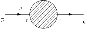
III Quark self-energy

We consider the loop correction to the quark propagator given by a diagram in Fig. 1, where blob represents a quantum correction of some loop level. This Green function is written in terms of the 1PE vertex function times external quark propagator with help of (II.42) (II.43),

$\displaystyle\left\langle q(p)\overline{q}(-p)\right\rangle_{1}=\frac{1-w_{0}^{2}}{ip\kern-4.30554pt/+(1-w_{0}^{2})m}\Sigma_{q}(p,m)\frac{1-w_{0}^{2}}{ip\kern-4.30554pt/+(1-w_{0}^{2})m}.$ (III.52)

The quark self energy $\Sigma_{q}(p,m)$ can be expanded in power of the external momentum $p$ and mass $m$ keeping the logarithmic dependence on them in coefficients,

$$\Sigma_{q}(p,m)=\Sigma_{0}+p_{\mu}\Sigma_{1\mu}+m\tilde{\Sigma}_{1}+p^{2}\Sigma_{2}+m^{2}\tilde{\Sigma}_{2}+mp_{\mu}\hat{\Sigma}_{2\mu}+{\cal O}(a^{2}),$$ (III.53)

where the coefficients $\Sigma_{0},\Sigma_{1\mu},\tilde{\Sigma}_{1},\Sigma_{2},\tilde{\Sigma}_{2},\hat{\Sigma}_{2\mu}$ are functions of $\log|p|,\log|m|$ and $p_{\mu}/m$,

$$\Sigma_{i}=\Sigma_{i}(\log|p|,\log|m|,p/m).$$ (III.54)

Here $p_{\mu}/m$ is introduced for generality. In (III.53) the first term represents the additive mass correction, the second and third term contribute to the quark wave function and multiplicative mass renormalization factors. The ${\cal O}(a)$ errors arise from the next three terms. The omitted terms give higher order errors of ${\cal O}(a^{2})$. The fact that $\Sigma_{0},\Sigma_{1\mu},\tilde{\Sigma}_{1},\Sigma_{2},\tilde{\Sigma}_{2}$ and $\hat{\Sigma}_{2\mu}$ are even functions of $(p,m)$ is important for our discussion. Our viewpoint is that if $\Sigma_{q}(p,m)$ is an odd function of $(p,m)$ the additive mass term and ${\cal O}(a)$ terms do not appear from the first in the expansion (III.53) and only the terms proportional to $p$ or $m$ survive to contribute to the corrections of wave function and mass multiplicatively. In this case, the leading discretization errors are ${\cal O}(a^{2})$.

In the following, we represent the self-energy in the form of loop integral as

$$\Sigma_{q}(p,m)=\int_{l_{1}\cdots l_{n}}\sigma(l_{1},\cdots,l_{n};p,m),$$ (III.55)

where $\int_{l_{1}\cdots l_{n}}$ is the shorthand of $n$ loop integral

$\displaystyle\int_{l_{1}\cdots l_{n}}=\int_{-\pi}^{\pi}\frac{d^{4}l_{1}}{(2\pi)^{4}}\cdots\frac{d^{4}l_{n}}{(2\pi)^{4}},$ (III.56)

which is invariant against the sign flip of $l_{1},\cdots,l_{n}$. We concentrate to show the oddness of $\sigma(l_{1},\cdots,l_{n};p,m)$ for the variables $l_{1},\cdots,l_{n},p,m$. If it is valid, $\Sigma_{q}(p,m)$ becomes odd function of $(p,m)$:

$\displaystyle\Sigma_{q}(-p,-m)$ $\displaystyle=$ $\displaystyle\int_{l_{1},\cdots,l_{n}}\sigma(l_{1},\cdots,l_{n};-p,-m)$ (III.57)
$\displaystyle=$ $\displaystyle\int_{l_{1},\cdots,l_{n}}\sigma(-l_{1},\cdots,-l_{n};-p,-m)$ (III.58)
$\displaystyle=$ $\displaystyle-\Sigma_{q}(p,m).$ (III.59)

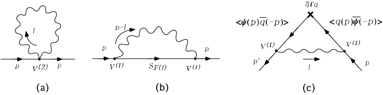
We begin by considering the one loop contributions, which are given by “tadpole” and “half-circle” diagrams of Fig. 2 (a) and (b) respectively. As was discussed in the above $\sigma(l;p,m)$ is given by multiplying the self energy of domain-wall fermion by the external quark line factors $[\xi_{e}L_{s}-\xi_{o}R_{s}]$, $[R_{s}\xi_{e}-L_{s}\xi_{o}]$ of the propagator (II.42) (II.43). Each diagram gives the following integrand,

$\displaystyle\sigma^{\rm tadpole}(l;p,m)$ $\displaystyle=$ $\displaystyle[\xi_{e}L_{s}-\xi_{o}R_{s}](p,m)V^{(2)}(-p,p)_{\mu\nu,st}[R_{t}\xi_{e}-L_{t}\xi_{o}](p,m)G_{\mu\nu}(l),$ (III.60)
$\displaystyle\sigma^{\rm half-circle}(l;p,m)$ $\displaystyle=$ $\displaystyle[\xi_{e}L_{s}-\xi_{o}R_{s}](p,m)V^{(1)}(-p,l)_{\mu,st}S_{F}(l,m)_{tu}V^{(1)}(-l,p)_{\nu,uv}G_{\mu\nu}(p-l)$ (III.61)
$\displaystyle\times$ $\displaystyle[R_{v}\xi_{e}-L_{v}\xi_{o}](p,m).$ (III.62)

We take summation over flavor index step by step from the left paying attention to the external quark line factor $[\xi_{e}L_{s}-\xi_{o}R_{s}](p,m)$ . A characteristic property of the factor is that an even and odd function is separated by the damping factor $L(p)_{s}$ and $R(p)_{s}$. We can see that this separation property is preserved under each steps in the diagram.

By using the commutation relation

$\displaystyle L(p)_{s}\gamma_{\mu}$ $\displaystyle=$ $\displaystyle\gamma_{\mu}R(p)_{s}$ (III.63)

and the form of internal fermion propagator in (II.25), the multiplication of the damping factor with the fermion propagator becomes,

$\displaystyle L(p)_{s}S_{F}(l,m)_{st}$ $\displaystyle=$ $\displaystyle f_{e}L(p)_{t}+h_{e}L(l)_{t}+f_{o}R(p)_{t}+h_{o}R(l)_{t},$ (III.64)
$\displaystyle R(p)_{s}S_{F}(l,m)_{st}$ $\displaystyle=$ $\displaystyle f^{\prime}_{e}R(p)_{t}+h^{\prime}_{e}R(l)_{t}+f_{o}L(p)_{t}+h^{\prime}_{o}L(l)_{t},$ (III.65)

where

$\displaystyle f_{o}$ $\displaystyle=$ $\displaystyle i\gamma_{\mu}\sin l_{\mu}X,$ (III.66)
$\displaystyle f_{e}$ $\displaystyle=$ $\displaystyle(W(l)-e^{\alpha(p)})X,$ (III.67)
$\displaystyle h_{o}$ $\displaystyle=$ $\displaystyle i\gamma_{\mu}\sin l_{\mu}Y_{2}+\frac{m(W(l)-e^{\alpha(p)})}{F(l)(e^{\alpha(l)}-e^{-\alpha(p)})}+\frac{me^{\alpha(p)-\alpha(l)}}{F(l)},$ (III.68)
$\displaystyle h_{e}$ $\displaystyle=$ $\displaystyle\frac{im\gamma_{\mu}\sin l_{\mu}}{F(l)(e^{\alpha(l)}-e^{-\alpha(p)})}+(W(l)-e^{\alpha(p)})Y_{1}+\frac{e^{\alpha(p)}}{F(l)},$ (III.69)
$\displaystyle f^{\prime}_{e}$ $\displaystyle=$ $\displaystyle(W(l)-e^{-\alpha(p)})X,$ (III.70)
$\displaystyle h^{\prime}_{o}$ $\displaystyle=$ $\displaystyle i\gamma_{\mu}\sin l_{\mu}Y_{1}+\frac{m(W(l)-e^{-\alpha(p)})}{F(l)(e^{\alpha(l)}-e^{-\alpha(p)})}-\frac{m}{F(l)},$ (III.71)
$\displaystyle h^{\prime}_{e}$ $\displaystyle=$ $\displaystyle\frac{im\gamma_{\mu}\sin l_{\mu}}{F(l)(e^{\alpha(l)}-e^{-\alpha(p)})}+(W(l)-e^{-\alpha(p)})Y_{2}-\frac{m^{2}e^{-\alpha(l)}}{F(l)},$ (III.72)
$\displaystyle X^{-1}$ $\displaystyle=$ $\displaystyle W(l)(e^{\alpha(p)}+e^{-\alpha(p)}-e^{\alpha(l)}-e^{-\alpha(l)}),$ (III.73)
$\displaystyle Y_{1}$ $\displaystyle=$ $\displaystyle A(l)\left[\frac{(1-m^{2})(1-We^{-\alpha(l)})}{F(l)(1-e^{-\alpha(p)-\alpha(l)})}-\frac{1}{1-e^{-\alpha(p)+\alpha(l)}}\right],$ (III.74)
$\displaystyle Y_{2}$ $\displaystyle=$ $\displaystyle A(l)\left[\frac{(1-m^{2})(1-We^{\alpha(l)})e^{-2\alpha(l)}}{F(l)(1-e^{-\alpha(p)-\alpha(l)})}-\frac{1}{1-e^{-\alpha(p)+\alpha(l)}}\right].$ (III.75)

Among several coefficients in (III.64) and (III.65), $f_{e},\ h_{e}$ and $h^{\prime}_{e}$ are even functions and $f_{o},\ h_{o}$ and $h^{\prime}_{o}$ are odd. Multiplication of the external line factor with the internal quark line becomes

$\displaystyle[\xi_{e}L_{s}-\xi_{o}R_{s}](p)S_{F}(l,m)_{st}$ $\displaystyle=$ $\displaystyle(\xi_{e}f_{e}-\xi_{o}f_{o})L(p)_{t}+(\xi_{e}h_{e}-\xi_{o}h^{\prime}_{o})L(l)_{t}$ (III.76)
$\displaystyle+$ $\displaystyle(\xi_{e}f_{o}-\xi_{o}f^{\prime}_{e})R(p)_{s}+(\xi_{e}h_{o}-\xi_{o}h^{\prime}_{e})R(l)_{t}.$ (III.77)

It should be noticed that the even-odd structure in which $L_{s}$’s have even coefficients and $R_{s}$’s have odd ones is preserved.

Multiplication with the interaction vertex $V^{(n)}$ is given by

$\displaystyle[\xi_{e}L_{s}-\xi_{o}R_{s}](p)V^{(1)}(p,k)_{\mu,st}=-ig(u_{\mu o}L_{t}+u_{\mu e}R_{t})(p),$ (III.78)
$\displaystyle\left[\xi_{e}L_{s}-\xi_{o}R_{s}\right](p)V^{(2)}(p,k)_{\mu\nu,st}=g^{2}(u_{\mu e}L_{t}+u_{\mu o}R_{t})(p)\delta_{\mu\nu},$ (III.79)
$\displaystyle\left[\xi_{e}L_{s}-\xi_{o}R_{s}\right](p)V^{(3)}(p,k)_{\mu\nu\lambda,st}=ig^{3}(u_{\mu o}L_{t}+u_{\mu e}R_{t})(p)\delta_{\mu\nu}\delta_{\mu\lambda},$ (III.80)

where $u_{\mu e}$ and $u_{\mu o}$ are even and odd function,

$\displaystyle u_{\mu e}(p,k,m)$ $\displaystyle=$ $\displaystyle\gamma_{\mu}\xi_{e}(p,m)\cos\frac{(-p+k)_{\mu}}{2}+ir\xi_{o}(p,m)\sin\frac{(-p+k)_{\mu}}{2},$ (III.81)
$\displaystyle u_{\mu o}(p,k,m)$ $\displaystyle=$ $\displaystyle\gamma_{\mu}\xi_{o}(p,m)\cos\frac{(-p+k)_{\mu}}{2}+ir\xi_{e}(p,m)\sin\frac{(-p+k)_{\mu}}{2},$ (III.82)

and we omitted the color factors. In general, the interaction vertex with even number of gluons $V^{(2n)}$ preserves the structure of damping factor and that with odd gluons $V^{(2n+1)}$ flips it so as to assigning odd coefficients to $L_{s}$’s and even to $R_{s}$’s.

After several multiplication in the diagram the external line factor from the left meets the other factor from the right and flavor index is summed over using the formula,

$\displaystyle L(p_{1})_{s}L(p_{2})_{s}$ $\displaystyle=$ $\displaystyle R(p_{1})_{s}R(p_{2})_{s}=\frac{1}{1-e^{-\alpha(p_{1})-\alpha(p_{2})}}\equiv C(p_{1},p_{2}),$ (III.83)
$\displaystyle L(p_{1})_{s}R(p_{2})_{s}$ $\displaystyle=$ $\displaystyle 0.$ (III.84)

We apply this scenario $\sigma^{\rm tadpole}(l;p,m)$. The left factor $[\xi_{e}L_{s}-\xi_{o}R_{s}](p,m)$ is multiplied to $V^{(2)}$ but this does not change the even-odd structure according to (III.79) and then meets the right factor and becomes an odd function,

$\displaystyle[\xi_{e}^{\prime}L_{s}-\xi_{o}^{\prime}R_{s}](p,m)[R_{t}\xi_{e}-L_{t}\xi_{o}](p,m)=-C(p,p)\left(\xi_{e}^{\prime}\xi_{o}+\xi_{o}^{\prime}\xi_{e}\right).$ (III.85)

In $\sigma^{\rm half-circle}(l;p,m)$, the flip of the even-odd structure occurs twice at each interaction vertex $V^{(1)}$ with (III.78). Multiplication with the fermion propagator does not change the structure as was shown in (III.77). Finally the left factor meets the right factor keeping the original structure and gives an odd function,

$\displaystyle[\xi_{e}^{{}^{\prime\prime}}L_{s}-\xi_{o}^{{}^{\prime\prime}}R_{s}](p,m)[R_{t}\xi_{e}-L_{t}\xi_{o}](p,m)=-C(p,p)\left(\xi_{e}^{{}^{\prime\prime}}\xi_{o}+\xi_{o}^{{}^{\prime\prime}}\xi_{e}\right).$ (III.86)

As a result, it is shown that $\sigma(l;p,m)$ is an odd function of $(l,p,m)$ at one loop level together with the fact that gluon propagator is an even function. Consequently the additive mass correction and ${\cal O}(a)$ errors vanish.

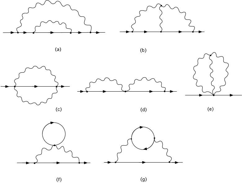
It is straightforward to extend the above discussion to two loop level. As examples we consider the diagrams of Fig. 3 (a), (b), whose integrands are

$\displaystyle\sigma^{(a)}(l_{1},l_{2};p,m)$ $\displaystyle=$ $\displaystyle[\xi_{e}L_{s}-\xi_{o}R_{s}](p,m)$ (III.87)
$\displaystyle\times$ $\displaystyle V^{(1)}(-p,l_{1})_{\mu}S_{F}(l_{1})_{st}V^{(1)}(-l_{1},l_{2})_{\rho}S_{F}(l_{2},m)_{tu}V^{(1)}(-l_{2},l_{1})_{\sigma}S_{F}(l_{1},m)_{uv}$ (III.88)
$\displaystyle\times$ $\displaystyle V^{(1)}(-l_{1},p)_{\nu}G_{\mu\nu}(p-l_{1})G_{\rho\sigma}(l_{1}-l_{2})[R_{v}\xi_{e}-L_{v}\xi_{o}](p,m),$ (III.89)
$\displaystyle\sigma^{(b)}(l_{1},l_{2};p,m)$ $\displaystyle=$ $\displaystyle[\xi_{e}L_{s}-\xi_{o}R_{s}](p,m)$ (III.90)
$\displaystyle\times$ $\displaystyle V^{(1)}(-p,l_{2})_{\mu}S_{F}(l_{2},m)_{st}V^{(1)}(-l_{2},l_{1})_{\nu}S_{F}(l_{1},m)_{tu}V^{(1)}(-l_{1},p)_{\rho}$ (III.91)
$\displaystyle\times$ $\displaystyle G^{(3)}(-p+l_{2},l_{1}-l_{2},p-l_{1})_{\alpha\beta\gamma}G_{\mu\alpha}(p-l_{2})G_{\nu\beta}(l_{1}-l_{2})G_{\rho\gamma}(p-l_{1})$ (III.92)
$\displaystyle\times$ $\displaystyle[R_{v}\xi_{e}-L_{v}\xi_{o}](p,m).$ (III.93)

There are four interaction vertices $V^{(1)}$ in $\sigma^{(a)}(l_{1},l_{2};p,m)$. Since the fermion propagator does not affect the even-odd argument, the even-odd structure of the left factor $[\xi_{e}L_{s}-\xi_{o}R_{s}](p,m)$ is flipped four times and finally meets with the right factor in the same form as in the tree level

$\displaystyle[\xi_{e}^{\prime}L_{s}-\xi_{o}^{\prime}R_{s}][R_{v}\xi_{e}-L_{v}\xi_{o}]$ (III.94)

and gives an odd contribution. Combined with the gluon propagator that is an even function, we can see $\sigma^{(a)}(l_{1},l_{2};p,m)$ is odd. On the other hand, there are three interaction vertices $V^{(1)}$ in $\sigma^{(b)}(l_{1},l_{2};p,m)$. This flips the even-odd structure of the left factor three times and the external quark line factor gives even contribution,

$\displaystyle[\xi_{o}^{{}^{\prime\prime}}L_{s}-\xi_{e}^{{}^{\prime\prime}}R_{s}][R_{v}\xi_{e}-L_{v}\xi_{o}].$ (III.95)

However, diagram $\sigma^{(b)}(l_{1},l_{2};p,m)$ also contains the three gluon self interaction vertex $G^{(3)}$ which is an odd function of $(l_{1},l_{2},p)$. Multiplying this term, the total loop integrand is an odd function. Confirmation of oddness for other remaining two loop diagrams is straightforward with the help of (III.77)-(III.80). We leave it to reader and just pick up three of them in Fig. 3 (c), (d) and (e) as examples. The above procedure is applicable to any quark self-energy diagram at any loop level and shows the oddness of the loop correction. The ${\cal O}(a)$ errors vanish for any diagrams.

In the end we have two comments on two loop diagrams Fig. 3 (f), (g) with fermion loop in the gluon polarization. The loop correction to the gluon polarization does not spoil the evenness of the gluon propagator because it is protected by gauge symmetry. Although it is almost trivial for the DWQCD from the same reason, we checked it explicitly at one loop level. This is accomplished by evaluating

$\displaystyle I_{\mu\nu}(l,p)$ $\displaystyle=$ $\displaystyle-{\rm tr}\left[V^{(1)}(-l,l+p)_{\mu}S_{F}(l+p,m)_{st}V^{(1)}(-l-p,l)_{\nu}S_{F}(l,m)_{ts}\right]$ (III.97)
$\displaystyle-{\rm tr}\left[V^{(2)}(-l,l)_{\mu\nu}S_{F}(l,m)_{ss}\right].$

Since the evenness is seen easily by substituting (II.25), (II.47) and (II.48), we omit the explicit calculation. The oddness of the three gluon self interaction vertex is also protected by gauge symmetry. The second comment is concerning the Pauli-Villars field needed to settle the infra-red divergence in fermion loop with infinite number of domain-wall fermion. The Pauli-Villars field is introduced as the $N$ flavor Wilson Dirac boson whose Dirac operator is the same as that of the domain-wall fermion except for the physical quark mass is changed to the cut-off order and opposite signature; $m\to-1$ [24] and it keeps the gauge invariance. This does not change the even-odd structure of the Feynman rules in pure gauge part.

IV Quark bilinear operator

We consider quark bilinear operators in the following form

$\displaystyle{\cal O}_{\Gamma}(x)=\overline{q}(x)\Gamma q(x),\qquad\Gamma=1,\,\gamma_{5},\,\gamma_{\mu},\,\gamma_{\mu}\gamma_{5},\,\sigma_{\mu\nu}.$ (IV.98)

We calculate the quantum correction to the Green’s function $\left\langle{\cal O}_{\Gamma}(x)q(y)\overline{q}(z)\right\rangle$ with external momenta $p,p^{\prime}$, As in the previous section we see that the external line is essentially written in terms of the quark propagator times damping factors in (II.42) and (II.43). Making use of this fact the full Green’s function for small external momentum becomes

$\displaystyle\left\langle(\overline{q}\Gamma q)\cdot q\overline{q}\right\rangle_{\rm full}=\frac{\left(1-w_{0}^{2}\right)Z_{w}Z_{2}}{ip\kern-4.30554pt/^{\prime}+(1-w_{0}^{2})Z_{w}Z_{m}^{-1}m}T_{\Gamma}(p^{\prime},p,m)\Gamma\frac{\left(1-w_{0}^{2}\right)Z_{w}Z_{2}}{ip\kern-4.30554pt/+(1-w_{0}^{2})Z_{w}Z_{m}^{-1}m},$ (IV.99)

where $T_{\Gamma}$ is the loop correction to the operator vertex and $Z_{2}$, $Z_{w}$, $Z_{m}$ are quantum correction to quark wave function, quark over all factor $w_{0}$ and mass whose explicit value is given in Ref. [23] at one loop. From the result of previous section, it is proven that the ${\cal O}(a)$ errors vanish automatically for $Z_{2}$, $Z_{w}$, $Z_{m}$. In this section we show that for $T_{\Gamma}$.

As in the previous section we expand the effective vertex $T_{\Gamma}(p,p^{\prime},m)$ in terms of external quark momentum $p,p^{\prime}$ and mass $m$ keeping the logarithmic dependence on them in coefficients, and then estimate the lattice artifact:

$$T_{\Gamma}(p^{\prime},p,m)=T_{0}+p_{\mu}T_{1\mu}+p^{\prime}_{\mu}T^{\prime}_{1\mu}+m\tilde{T}_{1}+{\cal O}(a^{2}).$$ (IV.100)

The coefficients $T_{0},T_{1}$ and $T^{\prime}_{1}$ are functions of $\log|p|,\log|p^{\prime}|,\log|m|,p/m,p^{\prime}/m$. $T_{0}$ contributes to the renormalization factor of the bilinear operator and following three terms are ${\cal O}(a)$ errors. If $T_{\Gamma}(p^{\prime},p,m)$ is an even function of $(p^{\prime},p,m)$, the ${\cal O}(a)$ errors vanish automatically. In the following we adopt the loop integral form as

$$T_{\Gamma}(p^{\prime},p,m)=\int_{l_{1}\cdots l_{n}}\gamma(l_{1},\cdots,l_{n};p^{\prime},p,m).$$ (IV.101)

$T_{\Gamma}$ is even provided the integrand $\gamma(l_{1},\cdots,l_{n};p^{\prime},p,m)$ is even function of $(l_{1},\cdots,l_{n},p,p^{\prime},m)$.

At one loop level, $\gamma(l;p^{\prime},p,m)$ is given by a diagram of Fig. 2(c) as

$\displaystyle\gamma(l;p^{\prime},p,m)$ $\displaystyle=$ $\displaystyle[\xi_{e}L_{s}-\xi_{o}R_{s}](p^{\prime},m)V^{(1)}(-p^{\prime},p^{\prime}+l)[R_{s}\eta_{o}+L_{s}\eta_{e}](p^{\prime}+l,m)\Gamma$ (IV.102)
$\displaystyle\times$ $\displaystyle[\eta_{o}L_{t}+\eta_{e}R_{t}](p+l,m)V^{(1)}(-p-l,p)[R_{t}\xi_{e}-L_{t}\xi_{o}](p,m)G_{\mu\nu}(l),$ (IV.103)

where the quark propagators (II.33) and (II.34) are used as internal lines, since “physical” fields are living in the operator vertex. Each internal line propagators contain damping factors $L_{s}$, $R_{s}$ and consideration of even-odd structure is carried for left and right hand side of fermion line independently. There is one fermion interaction vertex $V^{(1)}$ in each fermion lines of (IV.103) and flip of even-odd structure occurs once. This gives odd functions,

$\displaystyle[\xi_{o}^{\prime}L_{s}-\xi_{e}^{\prime}R_{s}][R_{s}\eta_{o}+L_{s}\eta_{e}]$ (IV.104)

for the left side line and

$\displaystyle[\eta_{e}^{\prime}L_{t}+\eta_{o}^{\prime}R_{t}][R_{t}\xi_{e}-L_{t}\eta_{o}]$ (IV.105)

for right side one making the total contribution even.

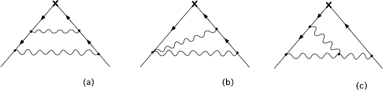
For two loop diagrams, we consider Fig. 4(a) as an example. There are two interaction vertices $V^{(1)}$ in each fermion line, where the even-odd flip occurs twice giving odd contribution. Therefore, the total contribution from the multiplication of them becomes even as expected. The above argument is valid for all other remaining two loop diagrams. For example estimation of diagrams in Fig. 4(b),(c) is an easy task and we leave it to reader.

V Conclusion

In this article, we made an estimation of the lattice artifacts in loop correction perturbatively for DWQCD in $N\to\infty$ limit. We studied quantum corrections to the Green function constructed from the physical quark field only. We revealed the even-odd structure of the diagrams in terms of the external quark momentum and mass.

With the help of the damping factors in the external quark propagator, we have shown to two loop level that the quark self-energy is definitely odd and the effective vertex of the quark bilinear operator is even. This means that the quark self-energy has neither additive mass correction nor ${\cal O}(a)$ errors, and ${\cal O}(a)$ errors in the effective vertex of the quark bilinear operator vanish automatically. Since our discussion can be extended to any loop diagram, we can show that ${\cal O}(a)$ errors do not appear for any diagram at any loop level in the same way. This is because the disappearance of them is deeply concerned with the hidden axial symmetry[18] of the DWQCD which was explicitly shown to exist in Ref. [21] for effective Lagrangian of the physical quark fields.

Acknowledgments

We thank S. Aoki for important suggestions and reading the manuscript. We also appreciate A. Ukawa, Y. Kikukawa, S. Ejiri, T. Izubuchi and K. Nagai for valuable comments and discussions. A part of this work is supported by the Grants-in-Aid for Scientific Research from the Ministry of Education, Science and Culture (No.2373). Y. T. is supported by Japan Society for Promotion of Science.

REFERENCES

  • [1] K. Symanzik, Nucl. Phys. B226 (1983) 187; 205.
  • [2] M. Lüscher and P. Weisz, Commun. Math. Phys. 97 (1985) 59, E:Commun. Math. Phys. 98 (1985) 433.
  • [3] B. Sheikholeslami and R. Wohlert, Nucl. Phys. B259 (1985) 572.
  • [4] G. Heatlie, C. T. Sachrajda, G. Martinelli, C. Pittori and G. C. Rossi Nucl. Phys. B352 (1991) 266.
  • [5] K. Jansen, C. Liu, M. Lüscher, H. Simma, S. Sint, R. Sommer, P. Weisz, U. Wolff, Phys. Lett. B372 (1996) 275.
  • [6] M. Lüscher, S. Sint, R. Sommer, P. Weisz, Nucl. Phys. B478 (1996) 365.
  • [7] M. Lüscher and P. Weisz, Nucl. Phys. B479 (1996) 429.
  • [8] S. Sint and P. Weisz, Nucl. Phys. B502 (1997) 251.
  • [9] D. Kaplan, Phys. Lett. B288 (1992) 342; Nucl. Phys.B (Proc. Suppl.) 30 (1993) 597.
  • [10] M. Golterman, K. Jansen and D. Kaplan, Phys. Lett. B301 (1993) 219.
  • [11] Y. Shamir, Nucl. Phys. B406 (1993) 90.
  • [12] V. Furman and Y. Shamir, Nucl. Phys. B439 (1995) 54.
  • [13] T. Blum and A. Soni, Phys. Rev. D56 (1997) 174; Phys. Rev. Lett. 79 (1997) 3595; Nucl. Phys. B (Proc. Suppl.) 63A-C (1998) 287.
  • [14] T. Blum, A. Soni and M. Wingate, Nucl. Phys. B (Proc. Suppl.) 73 (1999) 201; hep-lat/9902016.
  • [15] T. Blum, Nucl. Phys. B (Proc. Suppl.) 73 (1999) 167.
  • [16] P. Chen, N. Christ, G. Fleming, A. Kaehler, C. Malureanu, R. Mawhinney, G. Siegert, C. Sui, P. Vranas, Y. Zhestkov, Nucl. Phys. B (Proc. Suppl.) 73 (1999) 204.
  • [17] T. Izubuchi and K. Nagai, hep-lat/9906017.
  • [18] M. Lüscher, Phys. Lett. B428 (1998) 342.
  • [19] H. Neuberger, Phys. Lett. B417 (1998) 141; Phys. Lett. B427 (1998) 353.
  • [20] P. Hasenfratz, Nucl. Phys. B (Proc. Suppl.) 63 (1998) 53.
  • [21] Y. Kikukawa and T. Noguchi, hep-lat/9902022.
  • [22] S. Aoki and Y. Taniguchi, Phys. Rev. D59 (1999) 054510.
  • [23] S. Aoki, T. Izubuchi, Y. Kuramashi and Y. Taniguchi, Phys. Rev. D59 (1999) 094505.
  • [24] P. Vranas, Phys. Rev. D57 (1998) 1415.
Refer to caption
FIG. 1.: A quantum correction to the quark self-energy at some loop level . The blob represents the 1PE part.
Refer to caption
FIG. 2.: The one loop contributions to the quark self-energy;(a),(b) and the quark bilinear operator;(c).
Refer to caption
FIG. 3.: Typical contributions to the quark self-energy at two loop level.
Refer to caption
FIG. 4.: Typical contributions to the quark bilinear operator at two loop level.