CERN-TH/99-168
NORDITA-99/24HE
HIP-98-085/TH
hep-lat/9906028
{centering}
STATISTICAL MECHANICS OF VORTICES
FROM FIELD THEORY
K. Kajantiea,111keijo.kajantie@helsinki.fi,
M. Laineb,a,222mikko.laine@cern.ch,
T. Neuhausc,d,e,333neuhaus@physik.rwth-aachen.de,
A. Rajantief,444a.k.rajantie@sussex.ac.uk and
K. Rummukaineng,d,555kari@nordita.dk
aDept. of Physics,
P.O.Box 9, FIN-00014 Univ. of Helsinki, Finland
bTheory Division, CERN, CH-1211 Geneva 23,
Switzerland
cInstitut für Theoretische Physik E, RWTH Aachen, FRG
dHelsinki Inst. of Physics,
P.O.Box 9, FIN-00014 Univ. of Helsinki, Finland
eZiF, Univ. Bielefeld, D-33615 Bielefeld, FRG
fCentre for Theor. Physics, Univ. of Sussex,
Brighton BN1 9QH, UK
gNORDITA, Blegdamsvej 17,
DK-2100 Copenhagen Ø, Denmark
Abstract
We study with lattice Monte Carlo simulations the interactions and macroscopic behaviour of a large number of vortices in the 3-dimensional U(1) gauge+Higgs field theory, in an external magnetic field. We determine non-perturbatively the (attractive or repelling) interaction energy between two or more vortices, as well as the critical field strength , the thermodynamical discontinuities, and the surface tension related to the boundary between the Meissner phase and the Coulomb phase in the type I region. We also investigate the emergence of vortex lattice and vortex liquid phases in the type II region. For the type I region the results obtained are in qualitative agreement with mean field theory, except for small values of , while in the type II region there are significant discrepancies. These findings are relevant for superconductors and some models of cosmic strings, as well as for the electroweak phase transition in a magnetic field.
CERN-TH/99-168
NORDITA-99/24HE
HIP-98-085/TH
September 1999
1 Introduction
The continuum 3-dimensional (3d) U(1) gauge+Higgs field theory (scalar electrodynamics) is of interest for several reasons. First of all, it is the Ginzburg-Landau (GL) theory of superconductivity, believed to be applicable for low- and possibly also for some aspects of high- superconductors. Second, it is an often-used toy model for studying line-like cosmological topological defects, strings (adopting here the condensed matter terminology, we will mostly use the word vortex for these defects). Finally, the existence of topological excitations makes the model interesting also as a theoretical playground: much of the terminology related to our understanding of confinement, for instance, arises from superconductors. It is rather remarkable that for this theory, the topological observables of the continuum limit can be easily generalized in a gauge invariant way to the case with a finite lattice cutoff [1, 2].
In all these different contexts, it is of interest to ask how the behaviour of the system changes when an external magnetic field is added. In superconductors, an external magnetic field can be imposed experimentally, and it leads to the emergence of completely new phases, displaying for instance broken translational invariance. Due to magnetohydrodynamic diffusion, essentially homogeneous magnetic fields could also exist in cosmology and be relevant for the phase transitions appearing there; in any case, the core of each long U(1) vortex carries magnetic flux. From the theoretical point of view, a small external magnetic flux allows also to probe the topological properties of the zero-flux system in a gauge-invariant and systematic way.
In a previous paper [3], we showed how one unit of external magnetic flux can be imposed gauge-invariantly on the lattice, and how it can be used to determine non-perturbatively the free energy per unit length, i.e. tension, of a long vortex. The vortex tension thus defined was shown to constitute a gauge-invariant (but non-local) order parameter for the system, differentiating between the symmetric (“Coulomb”, “normal”) and broken (“Meissner”, “Higgs”, “superconducting”) phases. In the present paper, we study the case of a larger magnetic field. We show how to measure the free energy of a system of two or more vortices, thus seeing whether vortices attract or repel each other. This allows to divide the phase diagram into the region of type I and type II superconductors. We also increase the magnetic field further on and inspect whether this can lead to the emergence of new phases, triggered by the interactions of vortices, which are themselves macroscopic objects from the point of view of the original continuum quantum field theory.
In condensed matter physics vortices, of course, are a thoroughly studied topic (see, e.g., [4]–[7]). The emphasis is somewhat different, though. There the existence of a multitude of different scales and parameters implies that even the starting point, theory or model, is not uniquely known. The multitude of scales is related to the fact that one usually stays away from the immediate vicinity of the transition point, as a result of which the mean field approximation also often works very well. In particular, if one is studying the GL theory, one often approximates it by a simpler theory (the frozen gauge model, the XY model, etc.), using the narrowness of the fluctuation region as an argument. These arguments may be correct for physics, as it is only experiment which decides which effective theory is best, but they are not correct for the GL theory as such.
In the particle physics context, in contrast, given definite symmetry principles and the requirement of ultraviolet insensitivity, the form of the theory is uniquely defined; in the case of the U(1)+Higgs theory, keeping only relevant operators, it depends just on two dimensionless parameters. Moreover, close enough to the transition point, mean field approximation completely fails, and the theory is a genuine quantum field theory. It is quite striking that even for a simple theory such as U(1)+Higgs, the properties of the phase diagram are not yet completely known. We hope that studying the response of the system to an external magnetic field will shed new light on this issue.
Somewhat similar topics (with different methods and in 4d) were first studied with lattice simulations in [8]. External magnetic fields in the 3d SU(2)U(1) theory (corresponding to the Standard Model) were studied in [9], and in the 3d U(1) theory with fermions instead of scalars, in [10].
The plan of the paper is the following. In Sec. 2 we define the theory in the continuum and on the lattice, and review how an external magnetic field can be imposed and how the free energy related to vortices can be measured. In Sec. 3 we review the mean field results for the vortex and surface tensions and for the behavior of the system in an external magnetic field. In Sec. 4 we consider the full path integral and discuss the validity of the mean field approximation. In Sec. 5 we present our simulation results for the type I region, and in Sec. 6 for the type II region. We conclude in Sec. 7.
2 An external magnetic field and vortices on the lattice
The theory in continuum without external field.
The theory underlying our considerations is the U(1)+Higgs theory, corresponding to high temperature scalar electrodynamics on one hand [11]–[13] and to the Ginzburg-Landau model of superconductivity on the other [14]. It is defined by the functional integral
| (2.1) | |||||
| (2.2) |
where and . When all dimensionful quantities are expressed in proper powers of the scale , the theory can be parametrized by the two dimensionless ratios
| (2.3) |
where is the mass parameter in the dimensional regularization scheme in dimensions. For completeness, one may note that the standard dimensionful textbook coefficients [15] of the Ginzburg-Landau free energy and the dimensionless GL parameter are related to by
| (2.4) |
where is the fine structure constant and is an effective mass parameter. Note the huge numerical ratios entering here.
The theory on the lattice without external field.
The discretized lattice action corresponding to Eq. (2.2) is
| (2.5) | |||||
where , , , and where the lattice couplings are related to the continuum parameters and the lattice constant by [16] (for -corrections, see [17])
| (2.6) | |||
| (2.7) |
Note that we must use here the non-compact formulation for the U(1) gauge field, to avoid topological artifacts (monopoles) at finite (with the compact action one needs to go closer to the continuum limit to start with than as we have here, at least to ; see [12]).
The thermodynamical ensembles with an external field.
What we do in this paper is an extension to vortices of what was done for one vortex in [3]. Physically, we impose an external magnetic flux through the volume,
| (2.8) |
By convention, we have fixed the flux density as , and use an lattice with , , . On the average, after taking into account translational invariance, this flux density determines that , although in individual configurations the flux may not be evenly distributed. Together with the requirement of periodicity of observable quantities, Eq. (2.8) guarantees that there are vortices passing through the system, and we want to measure the free energy of such a configuration. Technically, fixing the flux is equivalent to multiplying the integrand in Eq. (2.1) by the delta-function
| (2.9) |
where the product has been written in a discretized form.
We shall use interchangeably the notation or for the free energy thus obtained, noting that and are related by Eq. (2.8) and that also depends on the parameters (see Eq. (2.3)) of the theory. Note that in our convention the free energy is dimensionless, , so that it corresponds to the free energy divided by temperature in standard terminology.
In a thermodynamic sense, fixing the flux means choosing a microcanonical ensemble. The results can also be transformed to the canonical ensemble ,
| (2.10) |
where is the volume of the system and is the external field strength. Technically, the canonical ensemble means multiplying the integrand in Eq. (2.1) by the factor
| (2.11) |
Imposing the magnetic flux on the lattice.
To impose a flux of units of on the lattice, we choose here to proceed as follows. We define a modified theory by
| (2.12) |
where the degrees of freedom are the periodic link angles
| (2.13) |
the periodic scalars , and
| (2.14) | |||||
Since, to leading order in ,
| (2.15) |
we have forced a flux of through the lattice; the stack of plaquettes parallel to the axis at the position is, in fact, a “Dirac string” carrying the flux in the direction.
A crucial fact now is that, due to the periodicity (2.13),
| (2.16) |
and thus the total flux through any plane vanishes identically. This implies that the flux must return through the system in the direction but now in a manner specified by the dynamics of the theory. This response is the object of the study here.
The Dirac string has been imposed by modifying one special plaquette on each plane leaving the part of the action involving scalars unchanged. When is an integer, integrating over all periodic field configurations makes the path integral (2.12) translation invariant. One could also, equivalently, impose the flux by making a non-periodic change in the boundary conditions for the link variable , as was done in Ref. [3]. Although translation invariance is broken with non-integer , the path integral (2.12) is well-defined, and non-integer values will indeed be used to interpolate between integers.
Finally, in principle one might also attempt to perform simulations with the canonical ensemble, as was done in [8]. In our case this can be accomplished by coupling an external field to the flux according to Eq. (2.11), i.e., adding a term to the action. This would promote to a dynamical variable, for which only integer values are allowed. However, in our case it would be very difficult to obtain an efficient update for . This is because the update is of semi-global nature: by performing it one attempts to make a large change in a configuration without any interpolation.
Measuring the free energy.
The aim now is to measure the change in the free energy caused by switching on the magnetic field, . Since one cannot measure the absolute value of the free energy on the lattice, we eliminate the unknown by taking a derivative with respect to and integrating back. This leads to the following result for the free energy per unit length (always relative to ):
| (2.17) | |||||
The subscript emphasises the fact that the expectation value is computed using the action (2.14) with the defect. We recall that we have chosen to express every dimensionful quantity in units of an appropriate power of . For instance, was made dimensionless in Eq. (2.17) by dividing it by .
Since is the quantity measured in our simulations, it is useful to have a feeling of its magnitude. It is essentially the expectation value of the stack of plaquettes at the position of the Dirac string. Eq. (2.14) for the first implies that the action is small for . This large negative contribution cancels the term in (2.17). This rough estimate can be improved by evaluating including only the gauge field in the action and using (2.16). The plaquettes are of two types: one at the string and not at the string. Using shift symmetries of the action one can then prove that
| (2.18) |
for all , which simply corresponds to , given by (2.8). In fact, the shift symmetries also hold for the full theory if = integer, so that Eq. (2.18) will give exactly when = integer. The behaviour of between integer values is seen from the numerical computations in Figs. 2(a-c).
Measuring the field strength.
In addition to the total free energy of flux units, we will be interested in the increase of free energy when the flux is increased by one unit, . Using and Eq. (2.10), this is, in fact, a measurement of :
| (2.19) |
3 Mean field results and
the determination of physical observables
In this section, we discuss the behaviour of the system at mean field level, and how this pattern can be employed in determining some of the physical observables of the full quantum theory.
One or two vortices.
In the mean field approximation the phase of the system is determined by the configuration that minimizes the action (2.2) under the boundary conditions imposed. In the bulk, for zero flux the system has two phases depending on ; a broken phase at and a symmetric phase at . The transition between the phases is of second order. In the broken phase the scalar and vector masses are
| (3.1) |
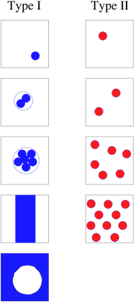
Assume now that the whole system is in the broken phase and ask what happens if one starts increasing the magnetic flux in the direction keeping the transverse area fixed (Fig. 1). This is concretely how our simulations will be organised.
Taking first one vortex line appears somewhere. By definition, the vortex tension is the free energy of this configuration divided by the length of the system in the -direction. In the mean field approximation, can be calculated by minimizing the action (2.2) with cylindrically symmetric boundary conditions. The result is [18]
| (3.2) |
where , () and ().
When is increased to , a difference between type I () and type II () appears: in the former case vortex lines attract and in the latter they repel each other. If we form the quantity
| (3.3) |
we thus expect that for type I,
| (3.4) |
due to the binding energy of two vortices. This also holds in the thermodynamic limit. For type II,
| (3.5) |
where the inequality holds on finite lattices and the equality in the thermodynamic limit. Thus is an order parameter for separating the type I and type II regions. In [3] it has been shown that itself, on the other hand, serves as an order parameter for the normal superconducting phase transition in this theory: it vanishes in the thermodynamic limit for .
The boundary between type I and II, , is mathematically very interesting since the classical equations of motion then simplify considerably. The dynamics of vortices can then be largely solved [19]. We shall not study this special case here.
3.1 Type I,
The general pattern.
Consider then type I and increase further. The lines parallel to first cluster on the plane as a 2d bubble (= 3d cylinder) of symmetric phase, but at some stage it becomes more favourable to form a slab (see Fig. 1). The cylinder and slab have interfaces separating the broken and symmetric phases. The tension of this interface can be written as
| (3.6) |
where is the extremal value of an integral already written down by Ginzburg and Landau. For small [20],
| (3.7) |
and one can analytically prove that vanishes for and becomes negative for . For intermediate values numerical methods have to be used [20, 21]. For the value of used in the type I simulations we find .
With continuously increasing the slab gets thicker. The broken phase region gets smaller and, ultimately, it reduces to a 3d cylinder of the broken phase, a hole in the magnetic field configuration. At some critical value of the flux, corresponding to a critical value of the field strength , the system goes entirely to the symmetric phase.
The detailed finite volume behaviour.
Consider now an inhomogeneous configuration in which the area is in the symmetric phase, and the area is in the broken phase with no . Let us denote the broken phase action density as
| (3.8) |
In the symmetric phase, the magnetic flux density is , and the action density is . If is the length of the boundary, the action per length is
| (3.9) |
where the three stages discussed above correspond to
These now have to be minimised for cylinder radii and the slab width (it was assumed that ) under the condition . The configuration corresponding to the minimum of then is the stable one. The minimisation is simplest for the slab: then
| (3.10) |
For the cylinders one has to minimise numerically, in general. However, an analytic result is obtained if the surface term is so small that it can be neglected in the minimisation, though it affects the value of . This is true if at the minimum value of . Then
| (3.11) |
For a slab configuration with , one obtains
| (3.12) |
Finally, for large one has a cylinder of broken phase within symmetric phase and
| (3.13) |
Comparing (3.11) and (3.12) one sees that a cylinder is favoured if
| (3.14) |
To see when the transition to the homogeneous symmetric phase takes place, one should compare with its free energy:
| (3.15) |
One sees, comparing (3.12) and (3.15), that this is smaller than even the slab free energy if
| (3.16) |
The transition to the symmetric phase will take place directly from the slab stage if the free energy of the 2nd cylinder stage is at larger than that of the slab:
| (3.17) |
Our simulations will, in fact, satisfy this condition. To see the stage with the cylindrical hole in the magnetic field configuration, one has to go to still larger lattices. This result is also confirmed by a full numerical minimization of Eq. (3.9).
The determination of and .
On the basis of the above equations we thus have a definite scenario for what happens when we increase the flux further from at finite volumes, and how this is related to the physical properties of the transition in the thermodynamical limit.
To see what Eq. (3.11) predicts for the measured (Eq. (2.19)), simply take a derivative of Eq. (3.11) with respect to (we recall that the relation of and is as in Eq. (2.8)). Then, for small the measurements should behave as
| (3.18) |
For (cf. Eq. (3.14)), the slab configuration dominates and leads to a constant plateau,
| (3.19) |
Finally, when , the system enters the Coulomb phase in which
| (3.20) |
Thus, we can determine from the plateau according to Eq. (3.19), and then from Eq. (3.18).
The determination of thermodynamical discontinuities.
We have here considered a system with a fixed , on which the magnetic field depends, but it may be more natural to move to the canonical ensemble in which is fixed and is allowed to fluctuate. This means simply inverting the relation of and . From this point of view, we simply have a standard first-order phase transition at , and when is below that, vanishes. The configurations with a cylinder or a slab describe the system on the transition line.
The thermodynamical discontinuities related to the first-order transition are directly given by the properties of the canonical free energy . The function is continuous across the phase transition, but its derivatives are not:
| (3.21) |
For fixed , the latent heat of the transition is defined as the discontinuity in the “energy” variable , obtained from by a Legendre transformation with respect to :
| (3.22) |
Note that for fixed , the identity leads to the Clausius-Clapeyron equation, relating the different discontinuities:
| (3.23) |
Thus it is enough to measure one of the discontinuities, and the curve . Below we choose to discuss (on finite volumes, instead of ). Finally, let us recall that at the mean field level Eq. (3.23) is satisfied through
| (3.24) |
3.2 Type II,
The determination of vortex tension and vortex interaction energy.
In the type I region, the vortex tension can be determined directly from Eqs. (3.2), (3.3). In the type II region, the issue is more involved, since there are large finite volume effects. Indeed, as discussed after Eq. (3.5), the difference between vanishes in the thermodynamical limit. However, this finite volume behaviour is well understood, and can be employed for the measurement of the properties of the vortex system.
The basic idea is that due to the repelling interaction, the vortices tend to form a vortex lattice in the type II region. In fact, due to the periodic lattice boundary conditions, even one vortex forms a square lattice with its periodic counterparts. Thus one can use finite size scaling with to study the interaction energy of two vortices. The method can be continued with , etc. Of course, this is not equivalent to a real vortex lattice, in which the distances between the vortices fluctuate; here the distance is fixed by the lattice size. When grows to much larger values so that the vortex separation is no longer determined by the lattice size, the vortices are instead supposed to form a physical (triangular) Abrikosov lattice.
Mean field theory offers an ansatz for the interaction energy: if is the physical distance between two vortices (it can be the lattice size in finite size scaling studies of or or the average distance between vortices, , at large ), then the interaction energy is [22]
| (3.25) |
where , is a Bessel function ( for ), and is the photon mass (in the broken phase). We have chosen to parametrize the prefactor in terms of the tension for later notational convenience, although, in fact, the physics of the prefactor is different from that in : the prefactor is only sensitive to asymptotic fields and the photon mass, and thus cancels between the mean field expressions for and . Let us also recall that the function appears in Eq. (3.25) because it determines the profile of a single vortex.
In the following, we will need an ansatz for the total free energy of a system of vortices forming either a square or a triangular lattice. We define the lattice sums
| (3.26) |
where the term is excluded and where the factor follows by requiring that the two lattices have the same number of sites within a large rectangular area. (From the point of view of a triangular lattice, it would be more natural to use a lattice geometry which is not rectangular but has , but we stick here to .) A numerical computation of the sums shows that they are very close to each other in the relevant range of ; this is the known fact that it is energetically difficult to distinguish between a square and a triangular lattice. This also means that it is quite difficult to differentiate between a lattice structure and a liquid phase, where the positions of the vortices fluctuate but have suitable average distances; we do not introduce a different ansatz for the liquid case.
We now parametrize the ansatz for the free energy of () type II vortices in an approximately triangular configuration measured on a square lattice () as
| (3.27) |
where we allow eventually to deviate from their mean field value. For , we have instead one vortex interacting with its replicas on an infinite periodic square lattice of period ,
| (3.28) |
and this can be used for the finite size scaling studies of the tension and the interaction energy . For two vortices the period is ,
| (3.29) |
which allows similarly to determine .
The determination of .
When the volume and the number of vortices are large, the question is what is their equilibrium configuration. Let us note first that at small enough , one is again in the Meissner phase just as in the type I region. The critical value for the transition to the vortex lattice phase can be obtained from Eq. (3.30): in the infinite volume limit, and
| (3.31) |
The magnetic flux increases continuously from zero, unlike for type I where there is a discontinuity.
Once , the vortices form a triangular Abrikosov lattice structure on the mean field level. Increasing further on, the lattice structure finally disappears when the energy squared corresponding to the lowest scalar Landau level becomes positive. This happens at
| (3.32) |
Note that the physics determining is quite different from that determining in the type I region, Eq. (3.8); at the expressions of course meet.
4 Fluctuations
The mean field approximation discussed above misses some essential features of the full path integral in Eq. (2.2). For example, for a vanishing magnetic field and for small (type I region) the transition is of first order, while for large (type II region) the precise characteristics of the continuous transition have not yet been completely understood. These fluctuation effects can be discussed perturbatively [14], but must eventually be studied with lattice simulations [12, 23]. There is no local order parameter to distinguish between the phases, but a number of non-local ones, e.g., the vector (photon) mass [12] and the vortex tension [3].
In general, the expansion parameters in the theory of Eq. (2.2) are, dimensionally, of the form (coupling constant)/(inverse correlation length “mass”). Choosing the scalar coupling and the scalar mass, corresponds to the standard Ginzburg criterion . In terms of the dimensionless variables , this means
| (4.1) |
Thus, for mean field theory to be valid, one simply has to be sufficiently deep in the broken phase. However, this is not the only expansion parameter: choosing instead, e.g., the vector coupling and the vector mass, , one gets a criterion which is more stringent at small ,
| (4.2) |
In any case, these are only qualitative criteria and the true size of fluctuation effects can only be established by numerical means. In many analogous models, the fluctuations change the mean field phase structure completely [24].
For a non-vanishing field , much new structure appears even on the MF level, as discussed above. What happens in the full theory can, in principle, be solved by the numerical methods presented here. Many simulations have been carried out with different simplified models (see, e.g., [25] and references therein), but it is not clear if the results should agree with the full locally gauge invariant U(1)+Higgs theory, preserving all relevant degrees of freedom.
Let us again consider the canonical ensemble (2.10), in which the magnetic field is fixed and is determined by the system. If the system is in the broken phase at , and is increased, the system eventually changes to the symmetric phase, which is characterized by a zero photon mass. For type I, the transition is of first order, and no other phases are believed to exist.
For type II, the magnetic field penetrates the system at strong enough fields, , via vortices, and the photon becomes massless. On the mean field level, the result would be a vortex lattice. However, it is clear that this picture changes when fluctuations are included. The interaction between the vortices becomes weaker when their distance increases and therefore at small enough magnetic field, the fluctuations will certainly destroy the lattice ordering. On the other hand, when the field is large, the vortices start to overlap and the cannot anymore be treated as interacting line-like objects. There is experimental evidence [7] as well as theoretical understanding in other models [4, 5, 6] that the lattice existing at intermediate fields, then melts into a vortex liquid phase, which is thought to be smoothly connected to the symmetric phase [5].
Therefore, it is an important question whether the lattice ordering predicted by the mean field theory really exists at all for intermediate magnetic fields in the U(1)+Higgs model. If there is no lattice phase, then the only true phase transition in the system is at , when the Meissner phase changes into a vortex liquid.

(a)

(b)

(c)
5 Simulations in the type I region,
The objective of the simulations in the type I region is to verify the qualitative picture discussed in Sec. 3, and to determine quantitatively the vortex tension , the critical field strength , and the surface tension . The simulations are carried out at one fixed and for . The lattice sizes are , . The number of flux units varies from 0 to about 33, corresponding to a range of from 0 to about 10. The mean field values of the scalar and vector correlation lengths are, at ,
and indicate that the approach to the continuum limit must be checked explicitly (since the vector correlation length is only of the order of the lattice spacing). From [26], we know that the tree-level estimates for the masses are reasonably good everywhere in the broken phase.
The numerical simulations, as presented here, were performed with the use of hybrid Monte Carlo update schemes for the gauge and the Higgs fields on parallel computer architectures. These were supplemented by simulations on workstation clusters, where the gauge fields were evolved using the more conventional -hit Metropolis update. A typical simulation for the calculation of the free energy change consumed (1…several) Monte Carlo sweeps of either algorithm. Such values of the statistics allow for relative errorbars at a few percent level in the measured quantity. Errorbars have been calculated with jack-knife methods and whenever necessary statistical error propagation was used. For a more detailed account of the algorithms, error calculation and the calculation of integrals we refer to [3].
All the measurements are based on measuring the function in Eq. (2.17). Since all the analysis is based on its integrals, i.e. free energies, we show only one example of itself in the type I region in Fig. 2(a); all other cases are very similar. Fig. 2(a) exhibits in a striking way all the features associated with increasing the number of flux units as described in Section 3. For smaller , contains a series of peaks between integer values . We know from Eq. (2.18) that at each integer . This value is reached within errorbars (not shown for clarity).
The peak in between the integer values represents the addition of one more vortex line, and the integral over the peak gives the additional free energy. The clustering of flux lines as a cylinder (a bubble on the 2-dimensional transverse plane) is seen as a decrease of peaks (Eq. (3.11)), and the slab as a relatively constant series of peaks (Eq. (3.12)). At some large the peaks suddenly disappear and the system goes over to the symmetric phase. At this point it may be illuminating to look also at the corresponding figures for the type II region in Figs. 2(b,c), which do not seem to show any abrupt transition.
5.1 Vortex tension and interaction energy from = 1, 2
We begin the study of the integrals of by considering them up to . The vortex tension was already studied in detail in [3], and a comparison of and carried out here is a measurement of vortex-vortex binding energy, which allows to differentiate between type I and type II regions. We choose and study finite size and finite lattice spacing effects in and . The values are obtained from Eqs. (3.2), (3.3).
In Fig. 3 we display and as a function of at and . The data shows no finite size effects. Fitting to a constant value one obtains
| (5.1) |
The fact that indicates an attractive force between the vortices.


To study the approach to continuum, we display in Fig. 4 and as a function of on a lattice at . We can use a single lattice size since finite volume effects were observed to be small. A dependence on is clearly seen and linear continuum extrapolations (the straight lines in the figure) result in
| (5.2) |
According to Eq. (3.2) the mean field value at this is so that . The magnitude of the scaling corrections is at the level of % for , somewhat smaller for , if the continuum results are compared with those at .
To study the dependence, we have measured and also at . The data again shows no apparent finite size effects. The result of a fit to a constant value is
| (5.3) |
corresponding to . Again, finite effects are expected to increase this number slightly.
Summarising this subsection, one observes clearly a finite tension difference caused by the attractive force between the vortices. There are also clear deviations from mean field which are largest close to the transition point, and actually quite sizable at .
5.2 Results for large
Data for (see Eq. (2.19)) is presented in Figs. 5(a–c) for three sets of parameter values, on a lattice, on a lattice, and on a lattice. We remind that this data contains integration over the successive peaks of such as those in Fig. 2(a).

(a)

(b)

(c)
In all the figures, in agreement with Section 3, one can see a region with a rapid variation (cylinder region), in which the data can be fitted to Eq. (3.18),
| (5.4) |
and a constant region (slab region), fitted to Eq. (3.19). The constant region gives the value of , the rapidly varying region the value of . After these values are known, one can compute the two transition values: in Eq. (3.14) for the cylinder slab transition and in Eq. (3.16) for the slab symmetric transition:
| (5.5) |
These are plotted in Figs. 5(a–c) as vertical lines. One observes that the flat section is approximately located within the -interval . For still larger lattices there would be a second cylinder stage (Eq. (3.13)), but now the condition (3.17) is satisfied and the transition takes place directly from a slab.
The horizontal lines in all three figures correspond to fits to the flat section. They determine the critical field , which in the mean field approximation is given by Eq. (3.8), . We obtain
| (5.6) |
The curves in the figures are fits to for values with the form (3.18) and they determine . At small one sees deviations from a spherical bubble shape and correspondingly the fits use data with , data with and data with . Compared with the value of from Eq. (3.6), the fit results in
| (5.7) |
Finally, let us consider the thermodynamical discontinuities discussed in Eqs. (3.21). We note that at finite volumes, is directly given by the value () where the system goes into the symmetric phase. However, there are large finite volume effects in this quantity (cf. Eq. (3.16)). In the infinite volume limit, we expect rather that , with the values of as given in Eq. (5.6). Through Eqs. (3.22), (3.23) and the curve from Eq. (5.6), this determines the latent heat.
Concluding this section, we observe that we have been able to determine , verifying that we are indeed in the type I region, as well as all the main thermodynamical properties of the first order transition from the Meissner phase to the Coulomb phase. Qualitatively, the mean field picture is valid, but on a quantitative level we observe a transition which is significantly stronger than at the mean field level, particularly for small .
6 Simulations in the type II region,
The simulations in the type II region have been carried out at , . The data for is mainly for the sectors of the theory to study vortex-vortex interactions and their finite size effects on periodic boxes. The data for is for large winding numbers and serves the purpose of determining the properties of the theory at a finite field .
As in the case of type I, all runs first compute but the analysis is based on its integrals. We thus present only two examples of in Figs. 2(b,c); the rest are similar and differ characteristically from those for type I in Fig. 2(a).
The analysis then proceeds as follows:
-
•
To have a rough picture of the spatial structure of a single vortex, we measure it in two ways: by explicitly measuring the profile of the vortex and by measuring the vector correlation length, which is expected to set the scale of a type II vortex at large distances.
- •
-
•
To confirm the understanding so obtained, we check whether the measured free energies of a many-vortex system, , can be reproduced. We also attempt to determine the phase of the system in the many-vortex region.
6.1 Vector field mass
To have information on the physical distance scales of the system, we shall first for and in the broken phase determine the vector field mass (the “photon mass”). We remind that this quantity is a (non-local) order parameter for the transition: it vanishes in the symmetric phase even after non-perturbative effects are taken into account [12]. Since we are in the type II region, the scalar mass is always heavier than and is thus subdominant at large distances (for explicit measurements of , see [12]).
The vector mass is determined as follows. We define the plane averaged correlator
| (6.1) |
choosing the lowest non-zero value for . We then measure and fit the correlator as
| (6.2) |
The frequency mode is related to via the lattice dispersion relation
| (6.3) |
We have measured for and for lattices of geometry and with . In Fig. 6, examples of the correlation functions are displayed. A fit in accord with Eq. (6.2) gives a perfect description of the data, and higher states appear to be strongly suppressed.
All values of determined here are collected in Table 1. For comparison, the numerical value of the mean field mass is also given in the table. The masses exhibit a mild and partly non-monotonous dependence on . This means that we are not yet at large enough volumes, particularly for . To have an estimate of the infinite volume values, we use a fit of the form
| (6.4) |
assuming finite size effects to be those of a massive theory. Other analogous fit forms give comparable results within errorbars. In case of a non-monotonous , only the two largest lattice sizes are included in this fit. The boldfaced numbers in Table 1 correspond to the extrapolations. They will be used in the following sections of the paper.

| -0.4 | 16 | 32 | 0.660(21) |
| -0.4 | 24 | 48 | 0.756(17) |
| -0.4 | 32 | 64 | 0.609(14) |
| -0.4 | 0.508(54) | ||
| -0.4 | MF | MF | 0.447 |
| -1 | 16 | 32 | 0.915(16) |
| -1 | 24 | 48 | 0.966(13) |
| -1 | 32 | 64 | 0.893(11) |
| -1 | 0.870(32) | ||
| -1 | MF | MF | 0.707 |
| -4 | 16 | 32 | 1.585(10) |
| -4 | 24 | 48 | 1.676(10) |
| -4 | 32 | 64 | 1.693(18) |
| -4 | 1.684(16) | ||
| -4 | MF | MF | 1.414 |
| -8 | 16 | 32 | 2.170(8) |
| -8 | 24 | 48 | 2.246(10) |
| -8 | 32 | 64 | 2.286(18) |
| -8 | 2.256(16) | ||
| -8 | MF | MF | 2.000 |
6.2 Profile of the vortex

The basic idea of our method of imposing a flux of on the system is to put a defect along an arbitrary line and let the system dynamically decide how it responds to this, where it places the vortices, etc. In the free energy measurement of a single vortex, its position never enters. How can one then measure the profile of a vortex, i.e., the distribution of the flux density on its planar cross section?
To do this one has to fix the position of the vortex. This can be done by making the infinitely long defect in Eq. (2.14) of finite length in the direction. This effectively places a monopole and an antimonopole at the ends of the defect and localises the response. Concretely, take a lattice and shift the plaquette values by for fixed values but only for values of . Then the monopoles are located at and , which gives a total distance between the monopoles of in the -direction. The Dirac string between the monopoles is again compensated for by a vortex, and the field profiles are measured at half-way distance between the monopoles, i.e., at .
Let be the distance from the center of the defect . Assuming rotational invariance we measure the statistical average of the quantity
| (6.5) |
Results are displayed in Fig. 7 for . We have also repeated the procedure for a lattice and the data at in Fig. 7 stem from simulations with that lattice size.
In physical units, we expect the vortex size to be related to the vector correlation length . We thus introduce the dimensionless variable
| (6.6) |
and we fit the large distance behavior of the vortex profile for values by the form
| (6.7) |
We find that the asymptotic distance behavior at is perfectly described by the fit. Thus the asymptotic profile is governed by the vector mass alone. In the cases the constant can be chosen to be exactly zero, while at it has a slightly positive value, which we suspect to be a finite size effect. Note that the mean field value for the scalar mass at exceeds the photon mass by a factor of two, so that its contribution can be neglected.
Clearly, this analysis is only valid if the distance between the monopoles is larger than the width of the vortex, . The distance should not be too large, either, or the fluctuations of the vortex spread the fields and in the limit of infinite separation, the field distribution becomes uniform. We estimate that this leads to a Gaussian probability distribution of width for the position of the center of the vortex, and therefore, if , this effect can be neglected. In our case guarantees that this is satisfied.
6.3 Vortex-vortex interactions for
As discussed in Sec. 3.2, a determination of , from Eqs. (3.2), (3.3) is subject to much larger finite size effects in the type II case than in the type I case. (For an explicit comparison, see Figs. 3, 8.) Thus, we have to employ the ansatz discussed in Sec. 3.2 to determine . We denote the finite volume values by .
All of our data for and at measured on cubic lattices () is shown in Fig. 8 as a function of the lattice size . The pattern is similar for other values of . We recall that the tensions (Eqs. (3.2),(3.3)) are obtained by measuring (Eq. (2.17)) and integrating (Eq. (2.19)) over one or the two first peaks of functions such as those in Fig. 2.

The data in Fig. 8 is then fitted with two free parameters, namely and according to the finite size scaling laws in Eqs. (3.28) and (3.29), using as determined in Sec. 6.1. The numerical value of the distance control variable is, for ,
| (6.8) | |||||
We include data with in the lattice sums in Eqs. (3.26). Typical finite size scaling studies in other lattice models use values of , but we have checked that our fit results are stable under further omission of small data. The fits for (such as the lower curve in Fig. 8) have at and at . The parameters are
| (6.9) |
where the mean field result is , and the numbers in the square brackets correspond to changing the (infinite volume) values of within the errorbars given in Table 1. For , the data is not good enough for determining , while for all values of , the errors from the uncertainty in are within the statistical errorbars. Both and give comparable values for the infinite volume extrapolation (see Fig. 8). It is quite impressive that such large finite size corrections are described so well by the fit. This is a clear indication of the fact that the interaction is indeed described by .
Consider then the approach to continuum, , of and . We choose . For a fixed lattice we determine and at and . Table 2 contains in its second and fourth column data for the measured quantities and , . This data is then extrapolated to infinite volume using the previous measurements of in Eq. (6.9) and in Table 1, and assuming the validity of (3.28) and (3.29). The extrapolations are given in columns and of Table 2. Note that we have assumed that , do not depend significantly on , and we use the same values for each ; this clearly introduces some extra -dependence, but it turns out that the outcome of this rough procedure is numerically quite satisfactory. The data somewhat scatters; at large values of autocorrelations within the Monte Carlo process are large.

| 1.0000 | 2.488(170) | 2.488(170) | 2.489(125) | 2.489(124) |
| .5000 | 2.385(179) | 2.385(179) | 2.457(131) | 2.457(131) |
| .2500 | 2.485(182) | 2.473(181) | 2.838(112) | 2.735(107) |
| .1666 | 2.428(232) | 2.312(221) | 3.248(198) | 2.656(162) |
| .1250 | 2.738(276) | 2.326(237) | 4.187(256) | 2.605(159) |
We display and as a function of in Fig. 9. The straight line fit (the curve in the figure) corresponds to the form
| (6.10) |
for and a similar one for . The fit results in
| (6.11) |
having . This value is completely compatible with the one determined in Eq. (6.9) at and thus we conclude that finite- corrections are small and apparently under control for the values of considered. Fig. 9 can be compared with that for the type I case, Fig. 4.
To summarize this subsection, we have verified that at , at finite volumes but for . Hence we are in the type II region. We then showed that the infinite volume extrapolations can in turn be extrapolated to a finite physical value in the continuum limit.
6.4 The vortex system at large
Consider then the case of large . As in the type I region, we plot from Eq. (2.19). Our main data is shown in Fig. 10, which contains the integrals over the peaks in , shown in Fig. 2.
A first-order phase transition means that behaves discontinuously as a function of . In the microcanonical picture, it would correspond to a region in which is constant, or more precisely, would exhibit similar finite-size effects as those discussed in Sec. 3.1. The only region where this might be the case, is at small (cf. Fig. 10(b)). If that turns out to be true, there is a first-order phase transition from or a small non-zero value, to some finite larger value of . In principle the transition could be one from a vortex liquid phase at such small that the distance between the vortices is large enough that the interaction cannot preserve the lattice structure, to the lattice phase; or, more likely in a finite volume, from a vortex lattice phase enforced by the periodic boundary conditions, to a vortex liquid phase where the vortices are so close to each other that the average fluctuations become larger than the average distance.

(a)

(b)

(c)
In order to check whether a lattice or a liquid phase is more likely, the data for is fitted to the ansatz in Eq. (3.30) with both a triangular (T) and a square (S) lattice. We remind that now the ansatz is for and that the distance control variable quantitatively is ()
where the numbers in the parentheses correspond to the lattice sizes used in Fig. 10. The fit is done for with a fixed interval , where , and . We consider and as free parameters in the fit. The results for the parameters are given in Table 3 and the fits are shown in Figs. 10(a,b).
| -4 | 16 | T | 0.91(06) | 1.26(2) | 0.32 |
|---|---|---|---|---|---|
| -4 | 24 | T | 0.90(05) | 1.27(2) | 0.09 |
| -4 | 32 | T | 0.88(04) | 1.31(1) | 0.33 |
| -4 | 48 | T | 0.96(14) | 1.31(4) | 0.18 |
| -4 | 16 | S | 0.91(06) | 1.25(2) | 0.31 |
| -4 | 24 | S | 0.91(05) | 1.26(2) | 0.08 |
| -4 | 32 | S | 0.89(04) | 1.30(1) | 0.30 |
| -4 | 48 | S | 0.96(15) | 1.31(4) | 0.18 |
| -8 | 16 | T | 0.81(05) | 1.22(1) | 0.42 |
| -8 | 20 | T | 0.78(05) | 1.26(2) | 0.79 |
| -8 | 24 | T | 0.93(10) | 1.19(3) | 0.24 |
| -8 | 16 | S | 0.82(05) | 1.22(1) | 0.38 |
| -8 | 20 | S | 0.79(04) | 1.25(2) | 0.74 |
| -8 | 24 | S | 0.93(10) | 1.18(3) | 0.24 |
To summarize the results for the parameters at different -values: for the vortex-vortex interaction parameter we have . There is only mild -dependence and the results are consistent with those at in Eq. (6.9). The mean field value (applicable in the dilute limit) is , independent of . The tension values of the fit at large are , . These values differ from the infinite volume tension as determined in the dilute limit in Eq. (6.9) by about 10 percent, which may well be a finite volume effect. Finally, the and lattice fits coincide within errorbars.
The fact that the and lattice fits work equally well and give consistent results, means that we are not sensitive to the average spatial distribution of the vortices. Thus, a vortex liquid phase cannot be excluded, either.
To get more information on the phase, let us then inspect the region of large . At and , the peaks in persist at all values of studied (see Fig. 2), and the field strength does not reach the mean field Coulomb phase value , corresponding to vanishing magnetization . On the mean field level the transition to takes place according to Eq. (3.32) at
| (6.13) |
which is shown in Figs. 10(a-c) as a solid line and is well within the studied range. However, we do not observe any structure around these values.
For the data set at , we have performed a finite size scaling study of at a large value of . Considering hypercubic boxes for values , we display data for as a function of in Fig. 11. The data differs from the mean field prediction and suggests an infinite volume extrapolation to a value . The fitted curve in the figure corresponds to a finite size scaling ansatz
| (6.14) |
with . Such power law finite size corrections are expected in a massless phase. The exponent could in principle be non-trivial, but we are currently not in the position to determine its value from the fit. In any case, it is clear that the deviation of the measured from the mean field value is not a finite size effect.

When is further increased, should finally approach the value , but achieving high enough is costly in computer time. The required value of can be reduced by, say, decreasing . As an example, the case is shown in Figs. 2(c) and 10(c). Here reaches within errorbars already at but the data is not good for any quantitative analysis. However, it illustrates an interesting point: contrary to what one might conclude on the basis of the plots for in Figs. 2(a,b), on finite lattices there are no cusps at integer values of ; in addition, can fall below the line . In fact, is obtained when positive and negative contributions cancel out.
In experiments with high-temperature superconductors [7] a weakly first-order phase transition has been found at a large magnetic field , and it has been interpreted as a melting transition of the vortex lattice. Like the transition we could imagine to observe at small , it would also show up in our data as a constant part in Fig. 10. Clearly, there is no sign of such a transition in our data, so if one exists in the U(1)+Higgs model at the value we have studied, the transition must be extremely weak. A much more natural conclusion seems to be that at least for the parameter values studied, the 3d U(1)+Higgs model does not have a vortex lattice phase as a thermodynamical state, but that the structure obtained at the mean field level is removed by thermal fluctuations. Thus we would be in the liquid phase all the time, and it just smoothly changes into the symmetric Coulomb phase. This is in agreement with the behaviour of as a non-local gauge invariant order parameter: there is only one “Meissner” phase at with , while for , vanishes.
7 Conclusions and outlook
In this paper, we have shown how the interactions of vortices can be studied non-perturbatively with lattice simulations, starting directly from field theory. We have shown that the interaction energy between two vortices is negative in the type I region and positive in the type II region, as expected from mean field (MF) theory. Moreover, increasing the magnetic field further on, we have shown that vortex interactions can lead to phases with different types of macroscopic structures.
The present simulations were carried out in a region in which one approaches the limits of validity of MF-theory. In superconductivity (see Eq. (2.4)) and MF-theory works very well. Our simulations span the range and we, indeed, find increasing deviations from MF.
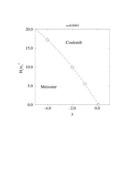
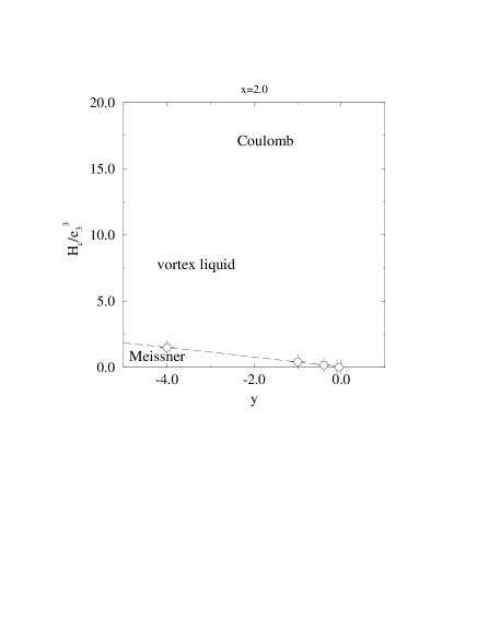
The regions of the phase diagram displaying Meissner, vortex liquid, vortex lattice, and normal Coulomb behaviour, have to date not been accurately mapped out in the full Ginzburg-Landau theory. We have demonstrated that the methods introduced here can answer these questions. Our present results and conclusions for the phase diagram in the -plane at are shown in Fig. 12. At , we find a first order phase transition in qualitative accordance with the MF estimate. However, the transition is much stronger than at the MF level, particularly for small (in fact, at the MF level the transition is of the 2nd order for , while the actual transition continues to be of the first order there). The vector field mass is non-zero only in the Meissner phase.
In the type II case and at , we observe only a single transition from the Meissner phase to a vortex liquid phase, which then smoothly turns into the Coulomb phase. This is in strong contrast to the MF prediction: we do not find any indications for a phase transition associated with the melting of a vortex lattice phase at large , so it seems natural to conclude that we are in the liquid phase all the time, and the fluctuations are strong enough to remove the lattice structure predicted at the MF level. On the other hand, we found very preliminary indications (Fig. 10(b)) that the transition to the vortex liquid phase at small might be of the first order. A possible interpretation for this behaviour is a finite volume effect associated with the ’melting’ of an unphysical lattice structure induced by the periodic boundary conditions, for a small number of flux quanta (in other words, a transition from a boundary-effect-dominated region to a bulk-dominated region).
Whether or not the theory in the thermodynamical limit allows for a physical triangular vortex lattice state in a strict sense at large values of , currently is an open question. It remains an algorithmic and computational challenge to extend the present simulations to the case of a truly macroscopic number of vortices.
One could imagine that techniques analogous to those introduced here can be developed for defects other than vortices, as well. For instance, in a theory with monopoles, one could fix the total magnetic flux emerging from the whole lattice volume. This would allow for a gauge-invariant non-perturbative study of the free energy of one monopole or of an ensemble of several monopoles.
Finally, let us note that the present techniques can be easily extended to the 3d SU(2)U(1)+Higgs theory, relevant for the cosmological electroweak phase transition in the Standard Model and many extensions thereof. In that case, an external magnetic field can represent physical (cosmological) reality, and can in principle lead to the emergence of phases analogous to the vortex lattice of type II superconductors [27]. Such phases might be relevant for baryogenesis and cosmology, and would thus be of considerable interest. We have observed that even in the U(1)+Higgs system where the lattice prediction is much more robust to begin with, fluctuations tend to remove the structure and result in a vortex liquid phase. This makes it quite understandable that in the SU(2)U(1) case no lattice structure (nor, in fact, a clear liquid-like behaviour) could be observed in the region of the parameter space studied so far [9], but one rather finds a symmetric phase.
Acknowledgements
We acknowledge useful discussions with T. Ala-Nissilä, M.A. Moore, A. Sudbø, Z. Tešanović and M. Tsypin. Most of the simulations were carried out with a Cray T3E at the Center for Scientific Computing, Finland, and with a number of workstations at the Helsinki Institute of Physics. Some simulations were also performed at NIC in Jülich. The total amount of computing power used corresponds to about 5 hours of a single Cray node’s capacity, i.e., floating-point operations. This work was partly supported by the TMR network Finite Temperature Phase Transitions in Particle Physics, EU contract no. FMRX-CT97-0122. A.R. was partly supported by the University of Helsinki.
References
- [1] J. Ranft, J. Kripfganz and G. Ranft, Phys. Rev. D 28 (1983) 360; M.N. Chernodub, M.I. Polikarpov and M.A. Zubkov, Nucl. Phys. B (Proc. Suppl.) 34 (1994) 256 [hep-lat/9401027]; M. Chavel, Phys. Lett. B 378 (1996) 227 [hep-lat/9603005].
- [2] A. Rajantie, Physica B 255 (1998) 108 [cond-mat/9803221]; K. Kajantie, M. Karjalainen, M. Laine, J. Peisa and A. Rajantie, Phys. Lett. B 428 (1998) 334 [hep-ph/9803367].
- [3] K. Kajantie, M. Laine, T. Neuhaus, J. Peisa, A. Rajantie and K. Rummukainen, Nucl. Phys. B 546 (1999) 351 [hep-ph/9809334].
- [4] G. Blatter, M.V. Feigel’man, V.B. Geshkenbein, A.I. Larkin and V.M. Vinokur, Rev. Mod. Phys. 66 (1994) 1125.
- [5] D.S. Fisher, M.P.A. Fisher and D.A. Huse, Phys. Rev. B 43 (1991) 130.
- [6] R.E. Hetzel, A. Sudbø and D.A. Huse, Phys. Rev. Lett. 69 (1992) 518.
- [7] E. Zeldov, D. Majer, M. Konczykowski, V.B. Geshkenbein, V.M. Vinokur and H. Shtrikman, Nature 375 (1995) 373; A. Schilling, R.A. Fisher, N.E. Phillips, U. Welp, D. Dasgupta, W.K. Kwok and G.W. Crabtree, Nature 382 (1996) 791.
- [8] P.H. Damgaard and U.M. Heller, Phys. Rev. Lett. 60 (1988) 1246; Nucl. Phys. B 309 (1988) 625.
- [9] K. Kajantie, M. Laine, J. Peisa, K. Rummukainen and M. Shaposhnikov, Nucl. Phys. B 544 (1999) 357 [hep-lat/9809004].
- [10] K. Farakos, G. Koutsoumbas and N.E. Mavromatos, Phys. Lett. B 431 (1998) 147 [hep-lat/9802037].
- [11] K. Farakos, K. Kajantie, K. Rummukainen and M. Shaposhnikov, Nucl. Phys. B 425 (1994) 67 [hep-ph/9404201].
- [12] K. Kajantie, M. Karjalainen, M. Laine and J. Peisa, Phys. Rev. B 57 (1998) 3011 [cond-mat/9704056]; Nucl. Phys. B 520 (1998) 345 [hep-lat/9711048].
- [13] J.O. Andersen, Phys. Rev. D 59 (1999) 065015.
- [14] H. Kleinert, Gauge Fields in Condensed Matter (World Scientific, 1989).
- [15] E.M. Lifshitz and L.P. Pitaevskii, Statistical Physics, Part 2, §45 (Pergamon Press, Oxford, 1980).
- [16] M. Laine and A. Rajantie, Nucl. Phys. B 513 (1998) 471 [hep-lat/9705003].
- [17] G.D. Moore, Nucl. Phys. B 493 (1997) 439 [hep-lat/9610013]; Nucl. Phys. B 523 (1998) 569 [hep-lat/9709053].
- [18] L. Jacobs and C. Rebbi, Phys. Rev. B 19 (1979) 4486.
- [19] P.A. Shah and N.S. Manton, J. Math. Phys. 35 (1994) 1171 [hep-th/9307165]; N.S. Manton and S.M. Nasir, hep-th/9809071.
- [20] J.C. Osborn and A.T. Dorsey, Phys. Rev. B 50 (1994) 15961 [cond-mat/9411015]; A.T. Dorsey, Ann. Phys. 233 (1994) 248.
- [21] E.V. Thuneberg, Phys. Rev. B 44 (1991) 9685.
- [22] L.M.A. Bettencourt and R.J. Rivers, Phys. Rev. D 51 (1995) 1842 [hep-ph/9405222].
- [23] B.I. Halperin, T.C. Lubensky and S.-K. Ma, Phys. Rev. Lett. 32 (1974) 292; C. Dasgupta and B.I. Halperin, Phys. Rev. Lett. 47 (1981) 1556; J. Bartholomew, Phys. Rev. B 28 (1983) 5378; Y. Munehisa, Phys. Lett. B 155 (1985) 159; P. Dimopoulos, K. Farakos and G. Kotsoumbas, Eur. Phys. J. C 1 (1998) 711 [hep-lat/9703004].
- [24] K. Kajantie, M. Laine, K. Rummukainen and M. Shaposhnikov, Nucl. Phys. B 493 (1997) 413 [hep-lat/9612006]; A. Hart, O. Philipsen, J.D. Stack and M. Teper, Phys. Lett. B 396 (1997) 217 [hep-lat/9612021]; K. Rummukainen, M. Tsypin, K. Kajantie, M. Laine and M. Shaposhnikov, Nucl. Phys. B 532 (1998) 283 [hep-lat/9805013]; K. Kajantie, M. Laine, A. Rajantie, K. Rummukainen and M. Tsypin, JHEP 11 (1998) 011 [hep-lat/9811004].
- [25] Z. Tešanović, Phys. Rev. B 51 (1995) 16204; Phys. Rev. B 59 (1999) 6449 [cond-mat/9801306]; A.K. Kienappel and M.A. Moore, cond-mat/9705151; cond-mat/9809317; A.K. Nguyen and A. Sudbø, Europhys. Lett. 46 (1999) 780 [cond-mat/9811149]; cond-mat/9907385.
- [26] M. Karjalainen and J. Peisa, Z. Phys. C 76 (1997) 319 [hep-lat/9607023].
- [27] J. Ambjørn and P. Olesen, Nucl. Phys. B 315 (1989) 606; Phys. Lett. B 218 (1989) 67; Nucl. Phys. B 330 (1990) 193; Int. J. Mod. Phys. A 5 (1990) 4525.