Abstract

The modelling of the ultraviolet contributions to the quark determinant in lattice QCD in terms of a small number of Wilson loops is examined. Complete Dirac spectra are obtained for sizeable ensembles of SU(3) gauge fields at $\beta=5.7$ on 6⁴, 8⁴ and 10⁴ lattices allowing for the first time a detailed study of the volume dependence of the effective loop action generating the quark determinant. The connection to the hopping parameter expansion is examined in the heavy quark limit. We compare the efficiency and accuracy of various methods - specifically, Lanczos versus stochastic approaches- for extracting the quark determinant on an ensemble of configurations.

1 Introduction

In a recent paper [1] we introduced a method for performing an unquenched Monte Carlo simulation in lattice QCD in which the infrared and ultraviolet modes of the quark fields are treated separately. The low eigenvalues (typically up to a cutoff somewhat above $\Lambda_{QCD}$) are exactly and explicitly calculated and included as a truncated quark determinant in the the update Boltzmann measure The remaining UV modes are included approximately by modelling the high end of the spectrum with an effective loop action involving only small Wilson loops. It was found that on small lattices (specifically, $6^{4}$ lattices at $\beta$=5.7) the accuracy of such a loop fit to the high end of the determinant was remarkably good- the $\chi^{2}$ per degree of freedom of a fit with loops of up to 6 links to the logarithm of the quark determinant, including all modes above 340 MeV was 0.23, while the typical excursion of the log determinant between uncorrelated configurations was on the order of 20. Of course, one expects that the accuracy of such a fit will decrease with increasing volume, and it is not clear that this approach will remain practical once lattices of physically useful size are reached. As an illustration, we note that recent studies of electromagnetic effects in lattice QCD [2] found that the finite volume effects from even the long-range electromagnetic effects were controllable on 12³x24 lattices at $\beta$=5.9. A 10³x20 lattice at $\beta$=5.7 has almost twice the physical volume, while the lattice discretization effects can presumably be substantially reduced by using clover improvement. Our aim in this paper is therefore to study the accuracy of effective loop action representations to infrared truncated quark determinants for various size lattices at $\beta$=5.7. We shall show that reasonably accurate representations of the UV contribution to the quark determinant in terms of a small number of Wilson loops are indeed possible on such physically useful lattices. To the extent that a small residual error in the loop representation of the ultraviolet part of the quark determinant contributes primarily to an overall rescaling of dimensional quantities such as ground-state hadron masses (which are dominated by quarks with a limited range of offshellness) such a representation should be perfectly adequate for dynamical spectrum calculations on moderately sized lattices.

Past studies of loop representations of the quark determinant [3, 4] (which typically focussed on the complete determinant, less accurately described by small loops) have been hampered by the difficulty of obtaining exact values for the quark determinant for a sufficiently large sample of independent gauge configurations. Stochastic methods [5, 6] can be applied to fairly large lattices but with limited accuracy, whereas the direct Lanczos approach [7] loses steam for lattices larger than about 12⁴. In this paper we have employed the Lanczos approach to obtain complete exact Wilson-Dirac spectra for sizeable ensembles of 6⁴, 8⁴ and 10⁴ lattices, allowing us to study in detail the volume dependence (Section 2) and quark mass dependence (Section 3) of the effective loop action fit to the truncated quark determinant at various infrared cutoffs. Technical details of the calculations, as well as a comparison of the computational burden of the exact Lanczos and stochastic approaches, are presented in Section 4.

2 Loop Actions for light quarks- volume dependence

The main difficulty we encounter in determining the accuracy of a loop representation for full or truncated quark determinants in lattice QCD lies in the computational effort required to extract complete spectra of the Wilson-Dirac operator for a sufficiently large sample of independent gauge configurations on lattices large enough to yield physically useful information. A variety of numerical tools, both exact and statistical, now exist for accomplishing this task. Technical details of the implementaion of these methods will be deferred to Section 4. In this section we present a detailed study of the volume and IR-cutoff dependence of loop fits to the quark determinant for ensembles of 75 6⁴ lattices, 75 8⁴ lattices and 30 10⁴ lattices at $\beta=$5.7 and $\kappa=$0.1685. For all of these configurations we have carried out a complete spectral resolution using the Lanczos methods discussed in Section 4, and identifying for each configuration all 15552 (resp. 49152, 120000) eigenvalues in the 6⁴ (resp. 8⁴, 10⁴) cases. Most of these calculations were performed on a 9 node Beowulf system running Linux.

The configurations used in this study were generated using the truncated determinant algorithm of [1]. In particular, the update measure included the contributions to the quark determinant from low eigenmodes of the hermitian Wilson-Dirac operator $\gamma_{5}(D_{W}-m)$ up to a cutoff $\Lambda_{QCD}$ (specifically, we chose a cutoff of 0.45 in lattice units, corresponding to about 490 MeV in physical units). This cutoff corresponds to the lowest 30 (15 positive and 15 negative) eigenvalues for the 6⁴ lattices, and to 120 (resp. 350) low eigenvalues for the 8⁴ (resp. 10⁴) lattices. It is reasonable to expect that, by including this infrared contribution in the simulation measure the low energy chiral structure is properly treated [1]. The essence of the task being addressed in this paper is then to determine the extent to which the remaining omitted ultraviolet modes can accurately be fit by a gauge-invariant loop expansion involving relatively few and simple loops. The loop actions discussed here will include only loops (or Polyakov lines) with up to 6 links, although the inclusion of loops with 8 links is completely straightforward in principle and would of course give a substantial increase in the accuracy of the fit.

Figure 1: 6 link closed loop contributions to $\cal{D}$

On a 6⁴ lattice with periodic boundary conditions, there are five independent gauge invariant contributions to $\cal{D}$=$\ln{{\rm det}(\gamma_{5}(D_{W}-m))}$ involving 6 links or less, corresponding to the plaquette (1x1 loop), here denoted $L_{1}(U)$, the length 6 Polyakov line traversing the full length of the lattice in any direction, $L_{2}(U)$, and 3 independent length 6 closed curves (denoted $L_{3,4,5}(U)$), illustrated in Fig.1. In the case of the 8⁴ and 10⁴ lattices there are only four such terms- the plaquette and the length 6 simply connected loops displayed in Fig. 1. In addition the fits contain a constant term which can be regarded as the lattice equivalent of the unit operator. We shall be studying the ultraviolet contribution to $\cal{D}$ in which the $n_{\lambda}$ lowest modes are omitted:

$${\cal D}(n_{\lambda})\equiv\sum_{i>n_{\lambda}}\ln{(|\lambda_{i}|)}$$ (1)

where $\lambda_{i}$ are the gauge-invariant eigenvalues of $(\gamma_{5}(D_{W}-m))$ enumerated in order of increasing absolute value. Denoting the approximate loop value of ${\cal D}$ by $S_{a}$ and the true value by $S_{t}$, the variance per degree of freedom of the fit, $\sigma^{2}$, is defined as:

$$\sigma^{2}=\sum_{n=1}^{n=nc}(S_{a}(n)-S_{t}(n))^{2}/(nc-np).$$ (2)

for $nc$ configurations and $np$ loop variables (including the constant term). (We note here that the terminology ”variance per degree of freedom” replaces the usual ”chi-squared per degree of freedom” as we are dealing with a dimensionless quantity without statistical errors.) In Figures (2-4) we show the accuracy of the best fit to ${\cal D}(n_{\lambda})$, for the cutoff corresponding to the actual simulation values - namely $n_{\lambda}=$30 (resp. 120, 350 for the 6⁴ (resp. 8⁴, 10⁴) lattices. The $\sigma^{2}$ is 0.24, 0.28 and 0.79 for the 3 cases studied . The very close matching of the loop action to the determinant values for $\sigma^{2}<$1 suggests that accurate dynamical calculations should be possible by replacing the UV part of the quark determinant by such a loop Ansatz.

Figure 2: 6 link fit to ${\cal D}_{30}$, 6⁴ lattices

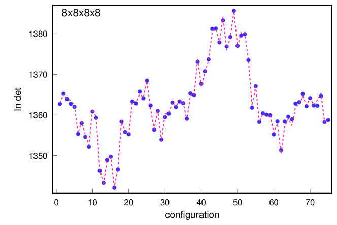
Figure 3: 6 link fit to ${\cal D}_{120}$, 8⁴ lattices

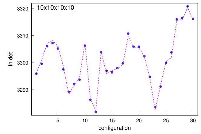
Figure 4: 6 link fit to ${\cal D}_{350}$, 10⁴ lattices

The accuracy of the loop fit to a truncated determinant is increased either by including longer loops or by raising the IR cutoff (which requires that more low eigenmodes be computed explicitly and included in the simulation). The variation with cutoff for the three different lattices studied is illustrated in Figure 5. The eigenvalue cutoff has been reexpressed as a physical lattice momentum, with the conversion performed using an average spectral density obtained by averaging the individual spectra for all lattices in the ensembles used. Loops up to length 6, together with Polyakov lines stretching across the lattice, have been included in the fit of the determinant.

Figure 5: $\sigma^{2}$ versus p${}_{min}({\rm lat})$ for 6⁴,8⁴ and 10⁴ lattices

The generic behavior is clear from Fig(5). The accuracy of the fit improves rapidly with increasing cutoff (initially, the variance decreases roughly like $e^{-Cp_{min}}$, where $p_{min}=|\lambda_{n_{\lambda}}|$ is the eigenvalue cutoff), reaching a small nonzero value. For the lattices studied,the minimum attained $\sigma^{2}$ was less than one in all cases, leading to the close matching of actual and loop fit determinant values visible in Figures 2-4. The $\sigma^{2}$ then fluctuates more or less randomly for further increases of cutoff around this value. This small nonzero contribution at fixed $\beta$ (increasing with the lattice volume) is due to higher dimension operators not included in the limited size loops in the fit and would presumably be reduced as the lattice $\beta$ is increased to push the system towards the continuum. The fluctuations are simply a reflection of the limited statistics of our relatively small ensembles- they become more visible at larger cutoff where the signal to background is reduced. This can also be seen by plotting the cutoff dependence of the $\sigma^{2}$ for the 6 link loop fits for the ensemble of 75 8⁴ lattices broken into three subensembles of 25 configurations each (Fig 6). At smaller cutoffs, strong infrared correlations extending over several lattices lead to fairly large differences in the $\sigma^{2}$ of the fits for small p_min, while at larger values of the cutoff, the size of fluctuations in each subensemble is comparable to the difference between the $\sigma^{2}$ for the different subensembles, suggesting that these fluctuations are statistical in origin.

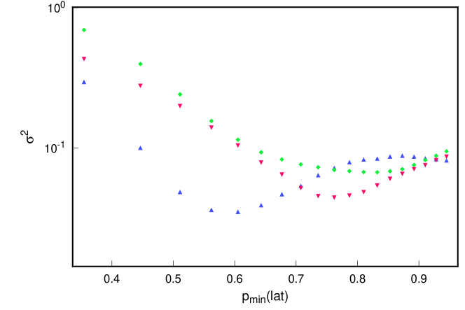
Figure 6: $\sigma^{2}$ versus p${}_{min}({\rm lat})$ for 3 ensembles of 25 8⁴ lattices

The accuracy of a simple loop representation for the ultraviolet part of the quark determinant, involving the contribution of a relatively small number of Wilson loop operators, depends on the fact that only a few independent gauge-invariant operators exist of mass dimension 4 or 6 [8]. On the other hand, the number of topologically distinguishable Wilson loops grows much more rapidly (in fact, exponentially) with the length of the loops. This results in very strong correlations between the values of distinct Wilson loop shapes over ensembles of independent lattices. For example, the single plaquette value is strongly correlated with the value of the 2x1 loop ($L_{3}$ in Figure 1). Thus, although the minimum $\sigma^{2}$ attainable for any given cutoff in link number is clearly only obtained by employing all Wilson loops up to the prescribed length, the actual coefficients of the individual loop values $L_{i}$ exhibit large variations from one subensemble to another for a given lattice volume, and also as the lattice volume is increased. On the other hand, if only truly independent operators are included, we should expect the coefficents (properly normalized for the overall lattice volume) to remain relatively constant as the lattice volume is increased at fixed $\beta$, reflecting the contribution of a definite set of low-dimension operators with expectation values approaching well-defined values in the infinite volume limit.

Cutoff $(1/a)$	Volume $N^{4}$	coefficients
$\Lambda_{QCD}$	$N$	constant	plaquette
0.00	6	-0.0225	0.0772
	8	-0.0209	0.0794
0.45	6	-0.0111	0.0695
	8	-0.0118	0.0699
0.56	6	-0.0043	0.0653
	8	-0.0048	0.0653

Table 1: Variation with volume of fit coefficients of link expansion of tr ln (Det) for various low eigenvalue cutoffs $\Lambda$.

This can be seen in Table 1, where we show the loop coefficients as a function of lattice volume for just the single plaquette operator obtained by minimizing the $\sigma^{2}$ with respect to a fit containing just a constant term (the unit operator) and the single plaquette loops (in operator terms, $F_{\mu\nu}^{2}$). The 10⁴ lattice results were not included because of the limited statistics available in this case (only 30 lattices as compared to 75 lattices for the 6⁴ and 8⁴ cases).

3 Quark determinant for heavy quarks- hopping expansion vs effective loop actions

The main physical difference between the behavior of the quark determinants for light and heavy quarks lies in the relative variance of the infrared and ultraviolet contributions. For light quarks, there are important fluctuations introduced both by the infrared modes, which incorporate the proper chiral behavior of the unquenched theory, and by the ultraviolet modes above $\Lambda_{QCD}$, which primarily renormalize the scale of the theory. Indeed, the latter are quantitatively dominant, but closely matched by an effective action involving only plaquettes or 6-link loops which for long distance physics reduces to an effective shift in the beta of the simulation. For heavy quarks, the density of the quark Dirac spectrum is much reduced in the infrared (which is cut off by the large bare quark mass), as are the fluctuations from the infrared modes below $\Lambda_{QCD}$, while the UV modes still have substantial variance, but again of a form which, as we shall show, can be accurately modeled by a simple loop action. The relative variance of the low and high end contributions of the (log) quark determinant is shown in Fig 7, where the IR/UV cut is placed at the 15 th (positive or negative) mode, roughly at $\Lambda_{QCD}$ for a 6⁴ lattice at $\beta$=5.7 (for the sake of visibility, an irrelevant constant vertical offset has been applied to bring the various contributions close to zero). For the heavier quark, $\kappa=$0.1500, there is comparatively little variance in the IR contributions, but large fluctuations in the UR part.

Figure 7: IR and UV contributions to quark determinants for light vs heavy quarks

The simplest approach one might take for the full quark determinant for heavy quarks employs the well-studied [9] hopping parameter expansion for $\cal{D}$=$\ln{(\gamma_{5}(D_{W}-m))}$, valid in the limit of small $\kappa$, i.e. large quark mass. In this section we examine the extent to which a truncated hopping parameter expansion can compete with the nonperturbative fitting of an effective loop action of the kind described in the preceding section. On a 6⁴ lattice with periodic boundary conditions, we saw previously that there are five independent gauge invariant contributions to $\cal{D}$ of order $\kappa^{6}$ or less, denoted $L_{i},1\leq i\leq 5$ above. The loop averages $L_{i}(U)$ on a given gauge configuration $\{U\}$ are normalized to give exactly one on the ordered configuration where all links are unity. Then a straightforward combinatoric exercise gives ($V$= lattice volume)

$$\cal{D}(U) = V(288\kappa^{4}L_{1}(U)-512\kappa^{6}L_{2}(U)+2304\kappa^{6}L_{3}(U)$$

$$+ 4608\kappa^{6}L_{4}(U)+1536\kappa^{6}L_{5}(U)+O(\kappa^{8}))$$

(Note that this computation gives an approximant to the full determinant, with no obvious way of implementing an IR/UV cutoff within the hopping parameter expansion.)

Unfortunately, the coefficients of higher order terms in the hopping parameter expansion grow fairly rapidly (the number of closed loops increases exponentially with the length of the loop) and the expansion converges slowly. For example, for $\kappa$=0.15, (with $\kappa^{8}$=2.6x10^-7 !) the average $\cal{D}$ over an ensemble of 30 configurations gives 172.4, while the hopping expansion gives 147.8. The discrepancy is nevertheless mainly due to a few low dimension operators which dominate the contribution of the longer loops, as is apparent from Fig 8. The hopping parameter expansion through 6th order tracks roughly the exact determinants apart from an offset (the identity operator). Of course, the nonperturbative fit including $L_{1-5}(U)$ does much better (the $\sigma^{2}$ is 0.112).

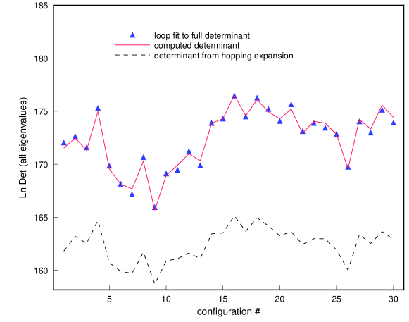
Figure 8: Full determinant, hopping parameter vs nonperturbative fit

We can improve the agreement of the truncated hopping expansion with the data by varying both the offset and the single plaquette component from the value of the $\kappa^{4}$ coefficient given in Eq (2). This amounts to including at least the lowest nontrivial dimension operator (dimension 4) arising from the longer loops (length 8 and higher). This fit is shown in Fig 9, in comparison with the unmodified hopping expansion result shifted only by a constant offset. The fit is certainly improved by optimizing the single plaquette component (the $\sigma^{2}$ is now 0.75) but clearly the nonperturbative fit of Fig. 8, in which all closed loops through length 6 are optimized, still wins by a substantial factor. We can conclude that even for quite heavy quarks, the hopping parameter expansion, though analytically available, is not competitive with a nonperturbative fit using even a small number of Wilson loops. Determining the coefficients in such a fit only requires the extraction of the determinant for a few typical configurations. We find that a sufficiently accurate determination of the loop coefficients can be obtained by calculating the spectrum on as few as 10 gauge configurations.

Figure 9: Hopping expansion fits, with offset vs with offset+plaquette

We pointed out earlier that the IR portion of the Dirac spectrum is relatively inert in the case of heavy quarks. One therefore expects that a nonperturbative fit with a few small loops should be accurate for heavy quarks, even if one insists on fitting the full determinant, as discussed above. Indeed, we saw above that the $\sigma{2}$ with a fit to the full determinant is 0.112 including loops up to length 6. The fit is still improved by excising the IR part of the spectrum, though not as dramatically as in the case of light quarks where the IR fluctuations require the inclusion of large loops. For $\kappa$=0.15, one finds for example that the $\sigma^{2}$ of a 5 loop fit decreases to 0.035, 0.026 and 0.019 when the lowest 30, 60 or 90 modes are excluded from the determinant.

4 Extracting the complete Dirac spectrum- explicit versus stochastic approaches

A fairly efficient method for performing a complete spectral resolution of the hermitian Wilson-Dirac operator was described some time ago by Kalkreuther [7]. One employs the usual Lanczos procedure, without reorthogonalization, pruning out the spurious eigenvalues by the Cullum-Willoughby procedure [10]. Typically the extraction of the complete Dirac spectrum requires (due to the inexact arithmetic) more Lanczos sweeps than the actual dimension (12$V$, where $V$ is the lattice volume), by a factor of 2-3. For example, on a 10⁴ lattice, the full spectrum is obtained after about 320000 Lanczos sweeps, as compared to the actual dimension of 120000. The convergence of the procedure is improved by starting from gauge-fixed configurations. (In spite of the fact that the spectrum is gauge-invariant, it appears that the presence of gauge noise can reduce the numerical stability of the Lanczos procedure.) Occasionally, spectral fluctuations lead to two eigenvalues which are almost degenerate, or a real eigenvalue almost degenerate with a spurious one, and the spectrum is found to be missing a small number of eigenvalues (note that the Lanczos procedure does not identify the degeneracy of the various eigenvalues). In an ensemble of 75 6⁴ lattices, the procedure missed a single mode in only two cases. For an ensemble of 20 10⁴ lattices, 3 eigenvalues were missed 5 times, 2 for 5 configurations, 1 for 6 configurations, and complete spectra were obtained for 4 configurations. Although the procedure can probably be tuned to reduce the frequency of missed eigenvalues, the general trend is nevertheless towards troublesome accidental degeneracies for larger lattices. Recently, we have found that the problem on larger lattices can be considerably ameliorated by a more careful retuning of the algorithm for identifying spurious eigenvalues- the resulting complete spectra agree completely with the reconstructed eigenvalues discussed below. Moreover, the convergence of the eigenvalues in the densest part of the spectrum occurs very rapidly as one reaches the end of the procedure, so that the spectrum of the tridiagonal matrix essentially consists of either spurious eigenvalues (easily identified by the Cullum-Willoughby procedure) or accurate converged eigenvalues. For example, with 320000 Lanczos sweeps on a 10⁴ lattice (120000 eigenvalues) one finds with a carefully tuned Lanczos calculation exactly 200000 spurious eigenvalues and 120000 converged eigenvalues, with the latter satisfying the set of exact sumrules discussed below to high accuracy (for a 10³x20 lattice with 240000 eigenvalues, complete spectra are obtained with 600000 Lanczos sweeps). The present tuning leaves about 3 orders of magnitude between the tolerance test for spurious eigenvalues (set at 10^-11) and the arithmetic precision (about 10^-14,15). For larger lattices where the volume and hence the maximum spectral density is a few orders of magnitude higher, we expect the Cullum-Willoughby procedure to misidentify some true eigenvalues as spurious, leading to incomplete spectra (as we indeed find if the tolerance parameter for spurious eigenvalues is set to 10^-10, for example).

In fact, in all cases mentioned above, incomplete spectra can be completely repaired with the aid of exact sum rules for traces of powers of the Wilson-Dirac matrix $H=\gamma_{5}(D_{W}-m)$. As we lose at most 3 eigenvalues, the lowest four sum rules suffice to determine all missing eigenvalues, with a spare relation left over for checking the accuracy of the reconstruction. One easily derives

$${\rm Tr}(H) = 0$$ (4)

$${\rm Tr}(H^{2}) = 12V(1+16\kappa^{2})$$ (5)

$${\rm Tr}(H^{3}) = 0$$ (6)

$${\rm Tr}(H^{4}) = 12V(1+64\kappa^{2}+(448-96<P>)\kappa^{4})$$ (7)

where the Wilson-Dirac operator $D_{W}-m$ in $H$ is normalized to be of the form $1+\kappa({\rm link\;\;terms})$, and $<P>$ in Eq(7) is the average plaquette value in the given configuration. A check of these sum rules on configurations where the entire spectrum has been successfully extracted gives ${\rm Tr}(H,H^{3})<$10^-7 while the quadratic and quartic sum rules are reproduced to at least eight significant figures. Repairing the incomplete spectra with these sum rules reveals, as expected, that the missing eigenvalues are either close to degenerate with each other or with a converged eigenvalue from the Lanczos procedure.

An alternative to the explicit spectral resolution of $H$, which is only really feasible for small to moderate sized lattices, is the stochastic approach developed by Golub and coworkers [5, 6], and applied by Irving and Sexton in their study [4] of loop actions for the quark determinant. Their formalism uses the close connection between the Lanczos recursion and Gaussian integration to generate rigorous lower and upper bounds to the diagonal matrix element $<v|f(A)|v>$ of any differentiable function $f(A)$ of a positive definite matrix $A$. The spectral sum giving this matrix element is transformed to a Riemann-Stieltjes integral and the usual quadrature rules (Gauss, Gauss-Radau, Gauss-Lobatto, etc.) applied to this integral can then be reexpressed in terms of a Lanczos recursion (for further details, we refer the reader to the paper of Bai, Fahey and Golub [6]). The use of alternative quadrature rules (in which information about the upper and lower limits of the spectrum is included in the Gaussian measure) does not seem to matter much in the application to the Wilson-Dirac matrix, although we have found that the Gauss-Lobatto version requires about 50% more Lanczos sweeps to achieve the same precision as the other quadrature rules. It is straightforward to generalize the arguments of [6] to show that the Lanczos estimates converge to the correct answer even for non-positive definite hermitian matrices (such as the hermitian Wilson-Dirac operator $H$), although the strict upper and lower bounds provided by the formalism no longer hold in the case $f(A)=\ln(A)$, as they depend on positivity of the derivatives of $f(A)$ over the entire spectrum. The rate of convergence of this procedure is impressive- for an 8⁴ lattice the estimate of $<v|\ln{|H|}|v>$ for a generic random vector $v$ with only 300 Lanczos sweeps is accurate to 7 places on a 8⁴ lattice, and to about 5 places on a 12³x24 lattice.

The Gaussian/Lanczos approach described above immediately leads to a stochastic method for estimating $\ln{\rm det}(|H|)=\sum_{i}<v_{i}|\ln{|H|}|v_{i}>$, where the sum extends over a complete orthonormal basis. Namely, one computes an average over a set of random vectors $|z_{i}>$ where each vector has components $\pm 1$ chosen at random:

$$\ln{\rm det}(|H|) = E(<z|\ln{|H|}|z>)$$ (8)

$$var(<z|\ln{|H|}|z>) = 2\sum_{i\not=j}|\ln{|H|}_{ij}|^{2}$$ (9)

We have checked that the choice of elements $\pm 1$ for the components of the random vectors is optimal, in the sense that the variance (8) obtained with this choice cannot be further reduced by an alternative choice of random variable. This procedure therefore gives an unbiased estimator for the full quark determinant, with errors that are purely statistical, decreasing as $1/\sqrt{N}$ with the number $N$ of random vectors used. Evidently the accuracy achieved for a given amount of computational effort is directly determined by the size of the offdiagonal matrix elements of $\ln{|H|}$. This is of course a very complicated functional of the gauge field for a general configuration. For the ordered configuration, however, $H$ can be explicitly diagonalized, and a straightforward computation yields

$$var(<z|\ln{|H|}|z>) = 4V\{\frac{1}{V}\sum_{k}\ln{(A(k)^{2}+B_{\mu}(k)B_{\mu}(k))}^{2}$$ (10)

$$- (\frac{1}{V}\sum_{k}\ln{(A(k)^{2}+B_{\mu}(k)B_{\mu}(k))})^{2}\}$$

where $A(k)=1-2\kappa\sum_{\mu}\cos{(k_{\mu})},B_{\mu}(k)=2\kappa\sin{(k_{\mu})}$, and $V$ is the lattice volume. In other words, the variance of the estimates (8) is exactly equal to the variance in the logarithm of the free quark lattice offshellness (as $A(k)^{2}+B_{\mu}(k)B_{\mu}(k)$ is just the lattice version of $k_{\mu}k_{\mu}+m^{2}$ in the continuum). For not too heavy quarks (it is easy to see that the variance (9) vanishes with $\kappa$) the number multiplying the lattice volume $V$ in (9) is of order unity, so the optimal stochastic procedure requires $N\simeq\sqrt{V}$ to determine $\ln{\rm det}(|H|)$ to within an additive error of order unity, assuming the free quark case as a rough guide. Explicit calculations show that the order of magnitude of the variance is indeed as given in (9). For example, the free quark formula (9) gives about 8x10³ for the variance on an 8⁴ lattice (choosing $\kappa$=0.12), while an actual run with 1000 random vectors on a nontrivial 8⁴ configuration ($\beta$=5.7, $\kappa$=0.1685) gives a variance of 9.7x10³, and a final result for the mean (log) determinant is 1224.0$\pm$ 3.1 (the error is obtained by taking the square root of the variance per data point). This should be compared with the exact value obtained from the complete spectral resolution carried out by the direct Lanczos approach described in the first part of this section, which was 1222.148. On a 12³x24 lattice at $\beta$=5.9, $\kappa=$0.1597, a typical configuration gave a variance of 8.0x10⁴, compared with 7.2x10⁴ from the free quark result (9) (again using $\kappa$=0.12 for the free case). An explicit evaluation with 820 random vectors gave a final result 8682$\pm$ 9.9 for the (log) determinant in this case.

We are now in a position to compare the computational efficiency of the direct and stochastic methods described above. The stochastic approach yields an estimate of the logarithmic determinant accurate to any fixed preassigned error with a computational effort growing like $V^{3/2}$, while the full Lanczos spectral resolution, which effectively determines the determinant to machine precision (actually, about eight significant figures), requires an effort of order $V^{2}$. However, the prefactors in each case render the Lanczos approach advantageous for small to moderate (say, 12⁴) lattices. For example, on an 8⁴ lattice, the complete spectral resolution requires on the order of 130000 applications of the “dslash” (lattice covariant quark derivative) operator, while the stochastic method would require about 10000 random vectors, each with 200 Lanczos sweeps- i.e a total of 2 million dslash operations- to reduce the error on the determinant to order unity (four significant figures). On the other hand, as discussed previously, on large lattices the direct Lanczos procedure is likely to fail as the machine precision will be inadequate to resolve the increasing number of accidental degeneracies due to the high spectral density. In this case the stochastic approach may be the only option for estimating the complete quark determinant.

5 Acknowledgements

The work of A.D. was supported in part by NSF grant 97-22097. The work of E.E was performed at the Fermi National Accelerator Laboratory, which is operated by Universities Research Association, Inc., under contract DE-AC02-76CHO3000. The work of H.T. was supported in part by the Department of Energy under grant DE-AS05-89ER 40518.

References

- [1] A. Duncan, E. Eichten and H. Thacker, Phys. Rev. D59, 014505(1999).
- [2] A. Duncan, E. Eichten and H. Thacker, Phys. Rev. Lett. 76, 3894(1996); Phys. Lett. B409, 387(1997).
- [3] J. C. Sexton and D. H. Weingarten, Phys. Rev. D55, 4025(1997)
- [4] A. C. Irving and J. C. Sexton, Phys. Rev. D55, 5456(1997).
- [5] G. Golub and G. Meurant, Stanford preprint SCCM93-07.
- [6] Z. Bai, M. Fahey and G. Golub, Stanford preprint SCCM95-09.
- [7] T. Kalkreuther, Comput. Phys. Commun. 95, 1(1996).
- [8] A. Patel and R. Gupta, Phys. Lett. B183, 193(1987).
- [9] I. Montvay and Munster, “Quantum Fields on a Lattice”.
- [10] J. Cullum and R. A. Willoughby, J. Comp. Phys, 44, 329(1981).