BNL–HET–99/2 Calculation of the strange quark mass using domain wall fermions

Abstract

We present a first calculation of the strange quark mass using domain wall fermions. This paper contains an overview of the domain wall discretization and a pedagogical presentation of the perturbative calculation necessary for computing the mass renormalization. We combine the latter with numerical simulations to estimate the strange quark mass. Our final result in the quenched approximation is 95(26) MeV in the ${\overline{\rm MS}}$ scheme at a scale of 2 GeV. We find that domain wall fermions have a small perturbative mass renormalization, similar to Wilson quarks, and exhibit good scaling behavior.

1 Introduction

The determination of the quark masses from first principles is an important task facing particle theorists today. The light quark masses are among the most poorly determined parameters of the Standard Model. The cause of the difficulty is the confining nature of QCD: quarks exist only in bound states. Furthermore, most of the mass of light hadrons is due to the energy of the color fields surrounding the quarks rather than the quarks themselves; therefore a nonperturbative treatment of QCD is required to connect the quark masses in the QCD Lagrangian with the spectrum of hadronic states measured experimentally.

Next–to–lowest order chiral perturbation theory ($\chi$PT) quite precisely predicts the ratios of quark masses [2] but cannot set the absolute scale. The most promising method of computing the light quark masses (i.e., $m_{u}$, $m_{d}$ and $m_{s}$) is lattice QCD. It has been suggested that QCD sum rules can be used to place fairly strict lower bounds on $m_{s}+m_{u}$ and $m_{d}+m_{u}$ by using analyticity conditions [3]; however, calculations of the values of the light quark masses from sum rules are thought to involve many uncertainties [4].

The feasibility of calculating the quark masses through Monte Carlo simulation of lattice QCD has been recognized since the early days of the field [5]. Most previous work utilized two formulations of lattice fermions: Wilson fermions which explicitly break chiral symmetry at finite lattice spacing and suffer from large discretization errors; and Kogut–Susskind fermions which maintain a remnant chiral symmetry, but badly break flavor symmetry and seem to have poorly converged weak–coupling expansions. Recently, Sheikholeslami–Wohlert (SW) fermions [6], an improvement of Wilson fermions, have also been used to compute the light quark masses [7, 8].

The usual method of computing the light quark masses on the lattice is the following. For fixed gauge coupling and various bare quark masses, one computes the pseudoscalar or vector meson mass from the exponential decay in Euclidean time of an appropriate correlation function. Using leading order $\chi$PT one extrapolates in the bare quark mass $m_{q}$ to where the meson mass takes on its physical value, then the corresponding value of the bare quark mass can be converted to the renormalized quark mass in any desired scheme. This method implicitly uses the vector Ward identity, so the difference $m_{q}-m_{c}$ is renormalized by $Z_{m}=Z_{S}^{-1}$, where $m_{c}$ is the bare quark mass corresponding to zero pion mass and $Z_{S}$ is the renormalization constant of the scalar density. Usually one converts the renormalized lattice quark mass to the continuum ${\overline{\rm MS}}$ regularization scheme by matching the weak coupling expansions of $Z_{S}$ in both schemes. Using this procedure the light quark mass $m_{l}\equiv(m_{u}+m_{d})/2$ and the strange quark mass $m_{s}$ may be computed independently, for example, using the pseudoscalar spectrum to fix $m_{l}$ and the vector spectrum to fix $m_{s}$. A comprehensive analysis of the light quark masses using this method appears in Ref. [9].

Recently several attempts have been made to remove some sources of uncertainty in the usual method. A large source of error in Wilson fermion calculations is the determination of the chiral limit; since they explicitly break chiral symmetry, Wilson quarks become massless at a nonzero critical bare quark mass, $m_{c}\neq 0$. One can avoid this error by using the axial Ward identity to fix the bare quark mass [10, 11]. One computes $\langle 0|\partial_{0}A_{0}|\pi\rangle$ and $\langle 0|P|\pi\rangle$, where $A_{\mu}$ is the local non-singlet axial vector current and $P$ the non-singlet pseudoscalar density, and then the quark mass is given by the ratio $\langle 0|\partial_{0}A_{0}|\pi\rangle/\langle 0|P|\pi\rangle$ and is renormalized by $Z_{m}=Z_{A}/Z_{P}$. Since the vector meson and baryon spectra cannot be used with this method, only one of either $m_{l}$ or $m_{s}$ may be fixed independently, the other is necessarily related by chiral perturbation theory.

Another large uncertainty enters into the matching between lattice and continuum regularizations. The typical scale at which this matching occurs is 2 GeV where the validity of WCPT is tenuous. In the case of Kogut–Susskind fermions, lattice WCPT is untrustworthy: next–to–leading order corrections can be 50–100% of the leading order term. Therefore, nonperturbative calculation of the renormalization factors is very desirable. Two methods are being explored presently which may remove the need for a perturbative expansion of the lattice theory [12], or push it to a very high energy scale at which the expansion parameter is much smaller [13]. Finally, the quenched approximation seems to give quark masses which are roughly 20% larger than unquenched quark masses [9]. Clearly this indicates that full QCD simulations are necessary for a precise calculation of light quark masses.

Presently no consensus has been reached regarding the values of the light quark masses, even within the quenched approximation. For example, using Wilson fermions and perturbative matching, the strange quark mass is 115(2) MeV when the kaon is used to fix the bare quark mass and 143(6) MeV when the $\phi$ meson is used [14], where the mass is defined in the ${\overline{\rm MS}}$ scheme at 2 GeV. Results using the SW action give a lighter strange quark mass of 95(16) MeV [8]. Furthermore, an exploratory nonperturbative determination of the quark mass renormalization agrees with the perturbative renormalization for the usual quark mass definition, but differs with the perturbative renormalization for the axial Ward identity definition [12]. Using the nonperturbative renormalization and the axial Ward identity, Ref. [12] finds a strange quark mass of 130(18) MeV. A more comprehensive presentation of the current status appears in Ref. [15].

In this paper, we employ a new fermion discretization to compute the light quark masses: domain wall fermions. Domain wall fermions utilize a fictitious extra (in this case, fifth) dimension in order to preserve chiral symmetry at nonzero lattice spacing; the chiral symmetries of the continuum are exactly preserved in the limit of an infinite fifth dimension [19, 57]. The idea originated in the context of chiral gauge theories. In Ref. [16], Kaplan constructed free lattice chiral fermions, without doublers, in $2k$ dimensions by considering Dirac fermions in $2k+1$–dimensions coupled to a mass defect in the extra dimension, or domain wall. For periodic boundary conditions in the extra dimension, an anti–domain wall also appears which supports $2k$–dimensional chiral fermions of the opposite handedness. Although the suitability of this approach for chiral gauge theories is still under intensive study, its usefulness for simulations of chirally symmetric vector gauge theories such as QCD now appears well established (for a review, see Ref. [17]).

Since the first suggestion that domain wall fermions offer a way to study chiral symmetry breaking of QCD [18, 19], considerable work has been done to assess the practicality of the method. In Ref. [18], a simplification of Kaplan’s original proposal is made for QCD simulations: half of the extra dimension is discarded, and the domain walls effectively become the boundaries of the extra dimension. For free field theory it has been shown that, for a range of the input parameters, a light four–dimensional mode of definite chirality is bound to one boundary and a similar mode of opposite chirality is bound to the other boundary; the mixing between the two modes is exponentially suppressed with the size of the extra dimension [19, 20, 21, 22]. Significant suppression of the mixing between the modes was also seen in nonperturbative simulations, but whether or not it is purely exponential remains an open question [23, 24, 25, 17]. Furthermore, the non–singlet axial Ward identity is reproduced, and predictions from chiral perturbation theory for the dependence of the pseudoscalar meson mass on the quark mass and for the kaon mixing parameter are satisfied [23, 24, 17]. Also, the expected behavior of $\langle\bar{q}q\rangle$ in the quenched approximation due to topological zero modes is reproduced [25, 26].

The paper is structured as follows: Section 2 introduces the details of the domain wall fermion action, Section 3 contains the results of the one–loop calculation of the massive quark self–energy, and Section 4 gives the details of our Monte Carlo simulations. In Section 5 we combine analytical and numerical results to give a value for the strange quark mass. Finally, we present our conclusions in Section 6 and include some details of our calculation in the Appendix.

2 Domain wall fermions

In this Section we review some properties of domain wall fermions in QCD, following the original boundary fermion variant by Shamir [18]. We take a pedagogical point of view and introduce notation and methods which will be relevant to our work later in this paper. We write down the action and the propagator, discuss the physics described by the light modes coupled to the boundaries, and mention previous work supporting the domain wall formulation of lattice QCD. For further details one should refer to the literature cited throughout the Section.

2.1 The action

On a lattice with spacing $a$, the domain wall fermion action is given by

$$-a^{4}\sum_{x,y}\sum_{s,s^{\prime}}\bar{\psi}_{s}(x/a)D_{s,s^{\prime}}(x/a,y/a)\psi_{s^{\prime}}(y/a),$$ (1)

where $x,y$ are four–dimensional Euclidean spacetime coordinates and $s,s^{\prime}\in[1,N_{s}]$ are coordinates in the fifth dimension. The Dirac operator can be separated into a four–dimensional part, $D^{\parallel}$, and a one–dimensional part, $D^{\perp}$:

$$aD_{s,s^{\prime}}(x,y)~{}=~{}aD^{\parallel}(x,y)\times\delta_{s,s^{\prime}}~{}+~{}\delta(x-y)\times aD^{\perp}_{s,s^{\prime}};$$ (2)

$x$ and $y$ have been rescaled to be dimensionless. The first term is the four–dimensional Wilson–Dirac operator with a mass term which is negative relative to the usual $4d$ Wilson fermion action:

$$aD^{\parallel}(x,y) = {1\over 2}\sum_{\mu}\Big{[}(1+\gamma_{\mu})U_{\mu}(x)\delta(x+\hat{\mu}-y)~{}+~{}(1-\gamma_{\mu})U^{\dagger}_{\mu}(y)\delta(x-\hat{\mu}-y)\Big{]}$$ (3)

$$+ (aM-4)\delta(x-y).$$

For $1<s<N_{s}$, the Dirac operator in the extra dimension is given by

$$aD^{\perp}_{s,s^{\prime}}=-\delta_{s,s^{\prime}}+{1\over 2}(1+\gamma_{5})\delta_{s+1,s^{\prime}}+{1\over 2}(1-\gamma_{5})\delta_{s-1,s^{\prime}}.$$ (4)

Note that the five–dimensional fermions are coupled to four–dimensional gauge fields which are identical at each $s$; i.e. the link matrices obey

$$U_{\mu,s}(x)~{}=~{}U_{\mu}(x) {\rm for} \mu\in[1,4],$$

$$U_{5,s}(x)~{}=~{}1 {\rm for} 1\leq s<N_{s}.$$ (5)

The boundary conditions in the fifth dimension are anti–periodic with a weight $am$ which, as we will see, is proportional to the $4d$ quark mass. The Dirac operator for the fifth dimension can be separated into its chiral components by the projectors, $P_{\pm}\equiv(1\pm\gamma_{5})/2$, such that

$$D^{\perp}_{s,s^{\prime}}~{}=~{}D^{\perp,+}_{s,s^{\prime}}P_{+}~{}+~{}D^{\perp,-}_{s,s^{\prime}}P_{-}.$$ (6)

In matrix notation,

$$aD^{\perp,+}_{s,s^{\prime}}~{}=~{}\left(\begin{array}[]{ccccc}-1&1&0&\ldots&0\\ 0&-1&1&\ldots&0\\ \vdots&\vdots&\vdots&\vdots&\vdots\\ 0&0&0&\ldots&1\\ -am&0&0&\ldots&-1\end{array}\right),\hskip 28.45274ptaD^{\perp,-}_{s,s^{\prime}}~{}=~{}\left(\begin{array}[]{ccccc}-1&0&\ldots&0&-am\\ 1&-1&\ldots&0&0\\ 0&1&\ldots&0&0\\ \vdots&\vdots&\vdots&\vdots&\vdots\\ 0&0&\ldots&1&-1\end{array}\right).$$ (7)

Since the perturbative calculation is simpler in (four–)momentum space, we Fourier transform the ordinary spacetime coordinates. The five–dimensional domain wall Dirac operator (2) becomes

$$aD_{s,s^{\prime}}(ap) = \Big{[}\sum_{\mu}i\gamma_{\mu}\sin ap_{\mu}+aM-\sum_{\mu}(1-\cos ap_{\mu})\Big{]}\delta_{s,s^{\prime}}+aD^{\perp}_{s,s^{\prime}}$$ (8)

$$= \sum_{\mu}i\gamma_{\mu}a\bar{p}_{\mu}\delta_{s,s^{\prime}}+W^{+}_{s,s^{\prime}}P_{+}~{}+~{}W^{-}_{s,s^{\prime}}P_{-}$$ (9)

where $a\bar{p}_{\mu}\equiv\sin ap_{\mu}$, and the $W^{\pm}$ are related to the $aD^{\perp,\pm}$ by

$$W^{\pm}_{s,s^{\prime}}~{}=~{}aD^{\perp,\pm}_{s,s^{\prime}}+\Big{[}aM-\sum_{\mu}(1-\cos ap_{\mu})\Big{]}\delta_{s,s^{\prime}}.$$ (10)

2.2 The mass matrix

The discrete extra dimension can be interpreted as a flavor space with $N_{s}-1$ heavy fermions and one light flavor [27]. In that framework, the $W^{\pm}$ in Eqn. (9) are mass matrices which govern the flavor mixing. One can have several physical pictures of how the mass hierarchy is maintained. The chiral symmetry is manifest in the domain wall picture; since the left– and right–handed modes are bound to opposite walls in the extra dimension and are separated by a distance $N_{s}$, so the chiral components can be rotated independently. The flavor space picture also provides insight. Ref. [28] relates the mass hierarchy in terms of a generalized see–saw formula. In fact, the Froggatt–Nielsen [29] mechanism allows one to establish an approximate conservation law which protects the light mass from large radiative corrections [28].

Let us examine the eigenvalues and eigenvectors of the tree–level mass matrix (in flavor space) for the action described above in Eqns. (1)–(7). Details are presented in Refs. [18, 21], and we repeat them in Appendix A.1 so that they may be extended to the one–loop case. Since the mass matrix is not hermitian, we diagonalize the mass matrix squared. Let $\Omega^{0}$ be the zero momentum limit of $W^{-}$ (10):

$$\Omega_{0}{}_{s,s^{\prime}}~{}=~{}\left(\begin{array}[]{ccccc}-b_{0}&0&\ldots&0&-am\\ 1&-b_{0}&\ldots&0&0\\ 0&1&\ldots&0&0\\ \vdots&\vdots&\vdots&\vdots&\vdots\\ 0&0&\ldots&1&-b_{0}\end{array}\right),$$ (11)

where $b_{0}\equiv 1-M$. Here and in the rest of the paper, we rescale $M$ so that it is dimensionless. As shown in Refs. [18, 21, 20], when $|b_{0}|<1$ the smallest eigenvalue of $\Omega_{0}\Omega_{0}^{\dagger}$ (and of $\Omega_{0}^{\dagger}\Omega_{0}$) is

$$(\lambda^{(1)})^{2}~{}=~{}(am)^{2}M^{2}(2-M)^{2}+O\Big{(}(am)^{4}\Big{)}+O\Big{(}(1-M)^{N_{s}}\Big{)}.$$ (12)

Therefore, the mass of the light mode, given by $\lambda^{(1)}$, has an additive renormalization which is suppressed as $N_{s}\rightarrow\infty$ for the range $0<M<2$. (We elaborate on this restriction on $M$ in the next Section and throughout the remainder of the paper.) For $|b_{0}|<1$ the eigenvectors of $\Omega_{0}\Omega_{0}^{\dagger}$ are given by

$$\phi_{s}^{(i)}~{}=~{}\left\{\begin{array}[]{ll}\sqrt{M(2-M)}~{}e^{-\alpha(s-1)}~{}\Big{(}{\rm sign}~{}b_{0}\Big{)}^{s-1}&i=1\\ \sqrt{{2\over N_{s}}}~{}\sin\bigg{(}{\pi(i-1)\over N_{s}}\Big{[}N_{s}+1-s\Big{]}\bigg{)}&i\neq 1\end{array}\right.$$ (13)

where the $i-$th eigenvector corresponds to eigenvalue $(\lambda^{(i)})^{2}$. The constant $\alpha_{0}$ is defined through

$$\cosh\alpha_{0}~{}=~{}{1+b_{0}^{2}-(\lambda_{0}^{(1)})^{2}\over 2|b_{0}|}.$$ (14)

Note that the light eigenmode in Eqn. (13) is exponentially concentrated at the $s=1$ boundary while the heavy ($i>1$) modes are not.

Once the eigenvectors of the mass matrix squared have been found, the Dirac operator can be diagonalized easily. Following Ref. [21] let us define unitary matrices $U^{(0)}$ and $V^{(0)}$ such that

$$U^{(0)}_{s,s^{\prime}}~{}\equiv~{}\phi_{s^{\prime}}^{(s)}\hskip 14.22636pt{\rm and}\hskip 14.22636ptV^{(0)}_{s,s^{\prime}}~{}\equiv~{}\phi_{N_{s}+1-s^{\prime}}^{(s)}.$$ (15)

Then the basis

$$\psi^{\rm diag}_{s}(p) \equiv U^{(0)}_{s,s^{\prime}}P_{+}\psi_{s^{\prime}}(p)+V^{(0)}_{s,s^{\prime}}P_{-}\psi_{s^{\prime}}(p)$$

$$\bar{\psi}^{\rm diag}_{s}(p) \equiv \bar{\psi}_{s^{\prime}}(p)P_{+}(V^{(0)}{}^{\dagger})_{s^{\prime},s}+\bar{\psi}_{s^{\prime}}(p)P_{-}(U^{(0)}{}^{\dagger})_{s^{\prime},s}$$ (16)

diagonalizes $DD^{\dagger}$ and $D^{\dagger}D$. Furthermore, the Dirac operator itself is diagonal in this basis, up to terms which vanish as $N_{s}\exp(-\alpha_{0}N_{s})$ [21, 22]:

$$\bar{\psi}(-p)D(ap)\psi(p) = \bar{\psi}^{\rm diag}(-p)\Big{(}V^{(0)}P_{+}+U^{(0)}P_{-}\Big{)}D\Big{(}P_{+}U^{(0)}{}^{\dagger}+P_{-}V^{(0)}{}^{\dagger}\Big{)}\psi^{\rm diag}(p)$$ (17)

$$= \bar{\psi}^{\rm diag}(-p)\Big{(}ia\hbox to0.0pt{/\hss}\kern-0.8pt\bar{p}~{}+~{}V^{(0)}W^{+}U^{(0)}{}^{\dagger}P_{+}~{}+~{}U^{(0)}W^{-}V^{(0)}{}^{\dagger}P_{-}\Big{)}\psi^{\rm diag}(p);$$

where the $V^{(0)}W^{+}U^{(0)}{}^{\dagger}$ and $U^{(0)}W^{-}V^{(0)}{}^{\dagger}$ are diagonal in $s,s^{\prime}$ [21]. Let us define $\chi\equiv\psi^{\rm diag}_{s=1}$, the eigenstate of the lightest eigenvalue of the mass matrix (squared). This mode has the effective tree-level action

$${\cal S}^{\rm tree}_{\rm eff}~{}=~{}a^{4}\int_{-\pi/a}^{\pi/a}{d^{4}p\over(2\pi)^{4}}~{}\bar{\chi}(-p)\Big{(}i\hbox to0.0pt{/\hss}\kern-0.8ptp~{}+~{}mM(2-M)\Big{)}\chi(p),$$ (18)

since $V^{(0)}W^{+}U^{(0)}{}^{\dagger}\Big{|}_{s=1,u=1}=U^{(0)}W^{-}V^{(0)}{}^{\dagger}\Big{|}_{1,1}=\lambda_{0}^{(1)}$ [21].

2.3 The propagator

The calculation of the tree–level fermion propagator $S_{F}$ proceeds similarly to the diagonalization of the mass matrix presented above. The final expression for the propagator is complicated, so we write it here schematically; it is written explicitly for the present action in [18, 21] and in Appendix B.1. As in Ref. [27] let us write the propagator as $S_{F}=D^{\dagger}/(DD^{\dagger})$ and project out its chiral eigenstates so that

$$S^{F}_{s,s^{\prime}}(p)~{}=~{}\Big{[}(-i\gamma_{\mu}\bar{p}_{\mu}\delta_{s,s^{\prime\prime}}+W^{-}_{s,s^{\prime\prime}})G^{R}_{s^{\prime\prime},s^{\prime}}P_{+}+(-i\gamma_{\mu}\bar{p}_{\mu}\delta_{s,s^{\prime\prime}}+W^{+}_{s,s^{\prime\prime}})G^{L}_{s^{\prime\prime},s^{\prime}}P_{-}\Big{]}$$ (19)

where $\bar{p}_{\mu}\equiv\sin p_{\mu}$, and $G^{R}$ ($G^{L}$) is the inverse of $D^{\dagger}D$ ($DD^{\dagger}$):

$$G^{R}_{s^{\prime\prime},s^{\prime}}~{}\equiv~{}\bigg{(}{1\over\bar{p}^{2}+W^{+}W^{-}}\bigg{)}_{s^{\prime\prime},s^{\prime}}~{}~{}{\rm and}~{}~{}G^{L}_{s^{\prime\prime},s^{\prime}}~{}\equiv~{}\bigg{(}{1\over\bar{p}^{2}+W^{-}W^{+}}\bigg{)}_{s^{\prime\prime},s^{\prime}}.$$ (20)

We give $G^{R}$ and $G^{L}$ explicitly in Appendix B.1, but let us mention their general behavior. The homogeneous solutions of

$$\Big{(}D^{\dagger}D\Big{)}_{s,s^{\prime\prime}}G^{R}_{s^{\prime\prime},s^{\prime}}=\delta_{s,s^{\prime}}~{}~{}{\rm and}~{}~{}\Big{(}DD^{\dagger}\Big{)}_{s,s^{\prime\prime}}G^{L}_{s^{\prime\prime},s^{\prime}}=\delta_{s,s^{\prime}}$$ (21)

are exponentials: $\exp(\pm\alpha(p)s)$. If $0<b(p)<1$ then the solutions are decaying exponentials; $\alpha(p)$ is real and defined through

$$\cosh\alpha(p)~{}=~{}{\bar{p}^{2}+1+b^{2}(p)\over 2|b(p)|},$$ (22)

where

$$b(p)~{}\equiv~{}1-M+\sum_{\mu}(1-\cos ap_{\mu}).$$ (23)

If $-1<b(p)<0$ then the solutions oscillate: $(-1)^{s}\exp(\pm\alpha(p)s)$, with $\alpha$ as in Eqn. (22). For $|b(p)|>1$ there is no longer a mode bound to the domain wall: the solutions of Eqn. (21) go like $\exp(\pm i\alpha(p)s)$ where $\alpha$ is now defined through

$$\cos\alpha(p)~{}=~{}{\bar{p}^{2}+1+b^{2}(p)\over 2b(p)},$$ (24)

Thus, $M$ must be in the range

$$0<M<2$$ (25)

in order for there to be a single massless fermion as $N_{s}\rightarrow\infty$. At greater values of $M$, “doubler” states in the other corners of the Brillouin zone become nearly massless. For example, the four states with one component of momentum near $\pi/a$ contribute, and so on in increments of 2 up to $8<M<10$ where again only a single state with all four momenta near $\pi/a$ exists. In fact the action is symmetric under the changes $M\to 10-M$ and $\psi_{s}(x)\to(-1)^{\sum_{\mu}x_{\mu}+s}\psi_{s}(x)$ so the physics of any region and the one reflected about $M=5$ are identical [30]. Henceforth, we concentrate our discussion on the single flavor theory near the origin of the Brillouin zone. Also note that the range of $M$ in Eqn. (25) is additively renormalized in the interacting theory, and we discuss this renormalization in detail in Sec. 3.2.

2.4 Summary of tree level properties

Let us emphasize the following points. For strictly infinite $N_{s}$ (and $m=0$) there is a massless right–handed fermion bound to the $s=1$ wall and a left–handed fermion bound to the anti–domain wall at $s=\infty$ [16]. For large, but finite, $N_{s}$ the mixing between the two chiralities is exponentially suppressed at tree level [18]. One describes a light 4–component Dirac fermion by coupling the two light modes with an explicit chiral symmetry breaking term $m$ [19]. Then the light Dirac fermion has a mass in the free theory equal to [18, 20]

$$am_{q}^{(0)}~{}=~{}M(2-M)\Big{[}am~{}+~{}(1-M)^{N_{s}}\Big{]}.$$ (26)

Therefore, neglecting exponentially small terms, domain wall fermions describe a light mode whose mass is multiplicatively renormalized. It also turns out that the light mode satisfies continuum–like axial Ward identities [19]. These features make domain wall fermions very attractive for simulating light quark physics, where chiral symmetry is crucial.

Another virtue of the domain wall formulation is that in the limit $N_{s}\to\infty$ the leading discretization errors for the $4d$ effective action are $O(a^{2})$. In the massless theory, any gauge invariant dimension–five operator with the required lattice symmetries can be written as a linear combination of the following two operators [6]:

$$O_{1} = \bar{q}~{}D^{2}~{}q$$ (27)

$$O_{2} = {i\over 2}\bar{q}~{}\sigma_{\mu\nu}F_{\mu\nu}~{}q$$ (28)

where $D^{2}$ is the second–order covariant derivative and $F_{\mu\nu}=[D_{\mu},D_{\nu}]$ is the field strength tensor. However, neither of these terms is invariant under a chiral transformation

$$q \rightarrow e^{i\epsilon\gamma_{5}}q$$

$$\bar{q} \rightarrow \bar{q}e^{i\epsilon\gamma_{5}}.$$ (29)

Since chirality violating effects have been shown to vanish as $N_{s}\to\infty$, the contributions of $O_{1}$ and $O_{2}$ to the effective action must be suppressed. In this sense, the domain wall fermion action is an $O(a)$–improved action [31, 24]. Even with an $O(a)$-improved action, $O(a)$ errors can enter into observables as the operators may require $O(a)$ improvement as well. However, such improvements would also violate chiral symmetry and, by the same argument as above, are suppressed as $N_{s}\to\infty$. Of course precise scaling tests are necessary to evaluate the extent of the improvement; although simulations to date [24], including the ones in this work, are consistent with these expectations.

3 Perturbative mass renormalization

In this Section we present our one–loop calculation of the quark mass renormalization. A renormalization factor is needed in order to match a lattice definition of quark mass to a continuum definition. We are also pursuing methods of computing renormalization factors nonperturbatively; however, that work is beyond the scope of this paper.

We compute the matching factor $Z_{m}(\mu,a)$ between a quark mass defined on a lattice with spacing $a$ to a continuum quark mass renormalized at momentum scale $\mu$:

$$m^{\overline{\rm MS}}(\mu)~{}=~{}Z_{m}(\mu,a)~{}m^{\rm LAT}(a).$$ (30)

$Z_{m}$ is computed by equating the one–loop continuum fermion propagator to the one–loop lattice fermion propagator. In this Section we present the calculation of the full five–dimensional self–energy, and then we discuss its effect on $M$ and $m$. The wavefunction renormalization has been computed already in Ref. [21]; we have extended that work to the massive case and present the full one–loop calculation here for clarity. Only the main points are made in the body of the Section, while more details are given in Appendix B.

3.1 Five–dimensional fermion self–energy

The fermion self–energy, $\Sigma(p,m)$, is given to one–loop order by the Feynman diagrams shown in Figure 1. We use $p$ to denote the external momentum and $l$ to denote the momentum in the loop integral. The tadpole graph has no fermion propagator in the loop, so it has trivial dependence on the fifth dimension, i.e. it is diagonal. On the other hand, the fermion in the loop of the half–circle graph may propagate in the fifth dimension (change flavor) while the gluon is unaffected. Therefore the half–circle graph has off–diagonal contributions in $s,s^{\prime}$ space.

Figure 1: One–loop fermion self–energy diagrams: the (a) tadpole and (b) half–circle graphs.

Even with the extra dimension, the steps of evaluating the half–circle graph are much like those for the calculation using Wilson fermions [34, 35]. First an integral which has the same infrared ($p\rightarrow 0$) limit is subtracted from $\Sigma(p,m)$ to cancel logarithmic divergences. The difference may then be Taylor expanded about zero lattice spacing. In the continuum limit, we neglect terms in the expansion which vanish as $a\rightarrow 0$; since the coefficients of $O(a)$ terms are exponentially suppressed with increasing $N_{s}$ the leading discretization errors are, in effect, $O(a^{2})$. The resulting expression can be arranged as follows:

$$\Sigma~{}=~{}{g^{2}C_{F}\over 16\pi^{2}}\Big{[}{1\over a}\Sigma_{0}+i\hbox to0.0pt{/\hss}\kern-0.8ptp\Sigma_{1}+m\Sigma_{2}\Big{]}.$$ (31)

After a lengthy calculation which is presented in Appendix B, these terms can be further subdivided into

$$\Sigma^{(0)}_{s,s^{\prime}} = I^{(0)}_{s,s^{\prime}}~{}-~{}2T\delta_{s,s^{\prime}}$$ (32)

$$\Sigma^{(1)}_{s,s^{\prime}} = L^{(1)}_{s,s^{\prime}}~{}+~{}I^{(1)}_{s,s^{\prime}}~{}-~{}{T\over 2}\delta_{s,s^{\prime}}$$ (33)

$$\Sigma^{(2)}_{s,s^{\prime}} = L^{(2)}_{s,s^{\prime}}~{}+~{}I^{(2)}_{s,s^{\prime}}$$ (34)

where the $L$ terms are proportional to $\ln a$, and the $I$ and $T$ terms are finite integrals to be computed numerically. We only need the renormalization of the lightest mode, so we delay further evaluation until we rotate the terms to the basis which diagonalizes the one–loop mass matrix. We should note, however, that the $I$ and $L$ terms are functions of $M$. Since $M$ becomes additively renormalized, this dependence is the source of a systematic uncertainty: what numerical value of $M$ should one use to compute $I^{(1)}$ and $I^{(2)}$? We will address this issue in Sec. 3.2. To summarize, the five-dimensional one–loop effective action is given by

$$\bar{\psi}_{s}(-p)\bigg{\{} a^{-1} \bigg{[}W^{+}P_{+}~{}+~{}W^{-}P_{-}~{}+~{}{g^{2}C_{F}\over 16\pi^{2}}\Big{(}I^{(0)}-2T\Big{)}\bigg{]}$$ (35)

$$+ i\hbox to0.0pt{/\hss}\kern-0.8ptp\bigg{[}1+{g^{2}C_{F}\over 16\pi^{2}}\bigg{(}L^{(1)}+I^{(1)}-{T\over 2}\bigg{)}\bigg{]}+m{g^{2}C_{F}\over 16\pi^{2}}\Big{(}L^{(2)}+I^{(2)}\Big{)}\bigg{\}}_{s,s^{\prime}}\psi_{s^{\prime}}(p).$$

3.2 Renormalization of $M$

We noted above (25) that in the free theory $M=0$ is the critical point where light modes begin to appear bound to the domain walls. The $1/a$ contribution from the self–energy graphs, $\Sigma_{0}$ given in Eqn. (32), shifts this value in the same way that the massless limit of Wilson–like fermions is shifted:

$$M=0~{}\to~{}M=M_{c},$$ (36)

where $M_{c}$ is the point at which the domain wall action first supports light chiral modes on the boundaries. If the tadpole contribution is dominant the shifts are identical since that graph is the same for domain wall and Wilson fermions.

Of course, the whole range of $M$ corresponding to light modes is renormalized when the coupling is non–zero, except that $M=5$ is a fixed point since the action is still symmetric under $M\to 10-M$ and $\psi_{s}(x)\to(-1)^{\sum_{\mu}x_{\mu}+s}\psi_{s}(x)$. For example, for numerical simulations it is helpful to know the optimal value of $M$ which minimizes the extent of the light mode in the fifth dimension. At tree–level the wavefunction corresponding to the zero mode bound to the $s=1$ domain wall is a $\delta$–function in the $s$–direction when $M=1$; i.e., $M=1$ is the optimal value for free domain wall fermions since the intrinsic quark mass arising from mixing of modes on opposite walls is minimized. However, simulations at $\beta\approx 6.0$ have shown that the optimal $M$ at which axial symmetries are preserved is somewhere around $1.7$ and that axial symmetries are poorly respected at $M=1.0$ [23, 24, 17].

The question now becomes, how is the whole range of $M$ renormalized? It cannot be a simple uniform shift since $M=5$ is a fixed point. If we consider only the tadpole contribution to the self–energy, the shift is approximately uniform in each region ($0<M<2$, $2<M<4$, $\ldots$), weighted by a factor

$$\sum_{\mu}(1-\cos{(p_{\mu})})\to 4,2,0,-2,-4$$ (37)

coming from the Wilson term. Surprisingly, this simple picture also describes the nonperturbative data well, as will be shown later in this paper. This tadpole–improved estimate of $M$ was originally proposed in Ref. [21].

Perturbatively, the shift of $M_{c}$ is given through the $a^{-1}$ terms in Eqn. (35):

$$M_{c}~{}=~{}-{g^{2}C_{F}\over 16\pi^{2}}\Sigma^{(0)}~{}=~{}-{g^{2}C_{F}\over 16\pi^{2}}\Big{(}I^{(0)}-2T\Big{)}.$$ (38)

$I^{(0)}=I^{(0)}_{s,s^{\prime}}$ is not diagonal in the extra dimension, the one–loop calculation of $M_{c}$ for the light mode involves rotating to the basis which diagonalizes the one–loop mass matrix. However, a reasonable first estimate for $M_{c}$ assumes the tadpole graph is numerically much larger than the contribution from $I^{(0)}$:

$$M_{c}^{\rm tad}~{}\equiv~{}{2g^{2}C_{F}T\over 16\pi^{2}},$$ (39)

where $T$ is given in Eqn. (56) and is numerically equal to 24.4. In Table 1 we give two values of $M_{c}^{\rm tad}$, each computed with different definitions of the strong coupling constant, $g^{2}_{V}(3.41/a)$ and $g^{2}_{V}(1/a)$. There is an obvious problem in deciding the relevant scale of this effect. In Section 5 we discuss the choice of coupling constant and scale in detail, but it is clear that a perturbative estimate of $M_{c}$ is not precise enough for our purposes. We note, however, that for a reasonable estimate of the renormalized coupling, the shift due to the tadpole agrees well with the above nonperturbative estimate.

Table 1: Values of $M_{\rm crit}$ estimated from the tadpole graph and computed with the 4–d Wilson fermion action.

	$\beta=6.3$	$\beta=6.0$	$\beta=5.85$
$M_{c}^{\rm tad}(3.41/a)$	0.676	0.754	0.812
$M_{c}^{\rm tad}(1/a)$	0.985	1.17	1.41
$\kappa_{c}^{W}$[37]	0.1519	0.1572	0.1617
$M_{c}^{W}$	0.708	0.819	0.908

Due to the above considerations, it is desirable to have a nonperturbative determination of $M_{c}$ since it appears in the definition of the lattice quark mass. A direct search for $M_{c}$ would be numerically prohibitive, so it is fortunate that there is a simple nonperturbative estimate available which originates from the overlap description of domain wall fermions [36] (thus it is exact only for $N_{s}\to\infty$). In this case a transfer matrix can be defined which describes propagation in the fifth dimension ${\cal T}=\exp(\gamma_{5}H^{W}(-M))$ where

$$H^{W}(-M)~{}\equiv~{}\gamma_{5}D^{\parallel}(-M)$$ (40)

is the ordinary $4d$ Hermitian Wilson–Dirac Hamiltonian with a mass term that is negative of the conventional one. $D^{\parallel}$ first supports exact zero modes as $M$ approaches a critical value $M_{c}^{W}$ defined by a vanishing pion mass. In this case ${\cal T}$ has a unit eigenvalue and propagation in the fifth dimension is unsuppressed. Thus $M_{c}$ for domain wall fermions corresponds to $M_{c}^{W}$ for Wilson fermions, usually given in terms of the hopping parameter, $\kappa_{c}^{W}$:

$$M_{c}^{W}~{}=~{}-\Bigg{(}{1\over 2\kappa_{c}^{W}}-4\Bigg{)}.$$ (41)

We can simply take $M_{c}=M_{c}^{W}$ from existing numerical simulations. In Table 1 we give the values of $\kappa_{c}^{W}$ computed in Ref. [37] and the corresponding value of $M_{c}^{W}$ which we use for the rest of this work.

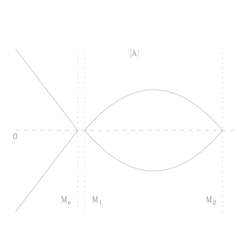
Figure 2: Expected spectrum of the Wilson–Dirac operator $D^{\parallel}$ as a function of $M$ (which is negative compared to the usual convention for Wilson fermions). There is a mass gap for $M<M_{c}$ and $M_{1}<M<M_{2}$, and no gap in the Aoki region $M_{c}<M<M_{1}$.

In Figure 2 we show schematically what the spectrum of the four–dimensional Wilson–Dirac operator should look like (with the domain wall convention for the sign of $M$) for the single flavor case. Ordinary Wilson fermion simulations are performed in the region $M<M_{c}$. while the domain wall fermion simulations have $M_{1}<M<M_{2}$. It has been conjectured by Aoki [38] that there is a range $M_{c}<M<M_{1}$ where there is no gap due to the spontaneous breaking of flavor and parity; evidence for the existence of this Aoki phase has been found in lattice QCD simulations [39] and analytically using an effective chiral Lagrangian [40] where the width of this phase, $M_{1}-M_{c}$, was found to be $O(a^{3})$. In the conventional picture (see Ref. [40] for a recent summary) the gap reopens after $M_{1}$ and closes again at $M_{2}$ when four of the doubler modes become massless.

The spectrum of the Hermitian Wilson–Dirac Hamiltonian has been studied in some detail in Ref. [41]. Many level crossings in the Hamiltonian were found uniformly in the region above $M_{1}$. These zeroes were related to small instanton-like configurations and are presumably related to the same lattice artifacts that give rise to so–called exceptional configurations [42]. If the density of these zero modes is non–zero in the large volume limit, then the gap is closed and domain wall fermions cannot exist: the entire allowed region of $M$ should then be in the Aoki phase. Since numerical evidence [23, 24, 25, 26] for the existence of domain wall fermions is quite strong, we infer that the density of these zeroes vanishes in the large volume limit (see Ref. [17] for more details), at least for the couplings relevant to present simulations. This is also consistent with the above studies of the Aoki phase. However, we also note that at some strong coupling the conventional picture is for the whole region to be in the Aoki phase, and at this coupling domain wall fermions cease to exist. The existence of the Aoki phase also reveals why the size of the extra dimension must increase as the coupling becomes stronger: as the gap gets smaller the size of the extra dimension must increase to maintain the same amount of suppression. We refer the reader to Ref. [28] for similar plausibility arguments on the behavior of domain fermions at strong and weak coupling.

In closing this section we emphasize that the simple replacement of

$$M~{}\rightarrow~{}\tilde{M}~{}\equiv~{}M-M_{c}^{W}$$ (42)

in the quark mass (26), though nonperturbative, is an ansatz which may or may not introduce $O(a)$ errors. Furthermore, $M$ cannot really be uniformly shifted, even piecewise, over the whole region. Nonperturbative effects such as instanton–like artifacts may be important (though these do seem to be more or less uniformly distributed above $M_{c}$). However, as previously mentioned, Eqn. (42) is a very good fit to our numerical data which we present in Sec. 4. Also the identification in Eqn. (41) is only exact in the limit $N_{s}\to\infty$. Again, simulations indicate this is a good approximation (see Ref. [17]).

3.3 Quark mass renormalization

In this Section we concentrate on the renormalization of the quark mass. We follow the method outlined in the case of the wavefunction renormalization [21]. The tree level quark mass was given in Sec. 2.2 by finding the smallest eigenvalue of the mass matrix squared, $\Omega_{0}\Omega_{0}^{\dagger}$. At one–loop level, the mass matrix is renormalized:

$$\Omega~{}\equiv~{}\Omega_{0}+g^{2}\Omega_{1}.$$ (43)

$\Omega_{0}$ is the tree–level mass matrix (11) and $\Omega_{1}$ is the one–loop correction given by the terms in (35)

$$\Omega_{1}~{}\equiv~{}{C_{F}\over 16\pi^{2}}\Big{(}\Sigma^{(0),-}+am\Sigma^{(2),-}\Big{)}.$$ (44)

where $\Sigma^{(j),\pm}\equiv\Sigma^{(j)}P_{\pm}$.

We rotate the fermion fields to the basis which diagonalizes the one–loop matrix $\Omega$

$$\psi^{\rm diag}_{s}(p) \equiv U_{s,s^{\prime}}P_{+}\psi_{s^{\prime}}(p)+V_{s,s^{\prime}}P_{-}\psi_{s^{\prime}}(p)$$

$$\bar{\psi}^{\rm diag}_{s}(p) \equiv \bar{\psi}_{s^{\prime}}(p)P_{+}(V^{\dagger})_{s^{\prime},s}+\bar{\psi}_{s^{\prime}}(p)P_{-}(U^{\dagger})_{s^{\prime},s}.$$ (45)

Then the terms which control the renormalization of the light fermion mode are as follows:

$$VW^{+}U^{\dagger}\Big{|}_{s=1,u=1} =UW^{-}V^{\dagger}\Big{|}_{1,1}~{}=~{} mM(2-M)$$ (46)

$$VI^{(0),+}U^{\dagger}\Big{|}_{1,1} =UI^{(0),-}V^{\dagger}\Big{|}_{1,1}~{}=~{} O(N_{s}b_{0}^{N_{s}})~{}\rightarrow~{}{\rm negligible}$$ (47)

$$UL^{(1),+}U^{\dagger}\Big{|}_{1,1} =VL^{(1),-}V^{\dagger}\Big{|}_{1,1}~{}\equiv~{} \tilde{L}_{1}$$ (48)

$$UI^{(1),+}U^{\dagger}\Big{|}_{1,1} =VI^{(1),-}V^{\dagger}\Big{|}_{1,1}~{}\equiv~{} \tilde{I}_{1}$$ (49)

$$VL^{(2),+}U^{\dagger}\Big{|}_{1,1} =UL^{(2),-}V^{\dagger}\Big{|}_{1,1}~{}\equiv~{} M(2-M)~{}\tilde{L}_{2}$$ (50)

$$VI^{(2),+}U^{\dagger}\Big{|}_{1,1} =UI^{(2),-}V^{\dagger}\Big{|}_{1,1}~{}\equiv~{} M(2-M)~{}\tilde{I}_{2}.$$ (51)

The results of Ref. [21] for $\tilde{L}_{1}$ and $\tilde{I}_{1}$ combined with our results for $\tilde{L}_{2}$ and $\tilde{I}_{2}$ are that

$$\tilde{L}_{1} = -2\int_{0}^{1}dx~{}x\ln\Big{(}{\pi\over az}\Big{)}^{2}~{}+~{}{3\over 2}$$ (52)

$$\tilde{L}_{2} = -4\int_{0}^{1}dx~{}\ln\Big{(}{\pi\over az}\Big{)}^{2}~{}+~{}4$$ (53)

$$\tilde{I}_{1} = -16\pi^{2}\int_{-\pi}^{\pi}{d^{4}l\over(2\pi)^{4}}~{}\Bigg{\{}{1\over 8\hat{l}^{2}}\sum_{\mu}\bigg{[}\sin^{2}l_{\mu}(\tilde{G}_{R}+\tilde{G}_{L})+2\cos l_{\mu}(b_{0}-b(l))\tilde{G}_{R}\Big{]}$$ (54)

$$+ \sum_{\mu}{\sin^{2}l_{\mu}\over 2\hat{l}^{4}}\Big{[}(b_{0}-b(l))\tilde{G}_{R}-\Big{(}2\cos^{2}{l_{\mu}\over 2}-\sum_{\nu}\cos^{2}{l_{\nu}\over 2}\Big{)}\tilde{G}_{L}+\hat{l}^{2}\tilde{G}_{R}\Big{]}\Bigg{\}}$$

$$+ 16\pi^{2}\int_{-\pi}^{\pi}{d^{4}l\over(2\pi)^{4}}~{}\Theta(\pi^{2}-l^{2})~{}{1\over l^{4}}$$

$$\tilde{I}_{2} = -16\pi^{2}\int_{-\pi}^{\pi}{d^{4}l\over(2\pi)^{4}}~{}{1\over\hat{l}^{2}}{1\over(1-e^{-\alpha(l)}b_{0})^{2}}~{}\Bigg{[}\bar{l}^{2}\sum_{\mu}\cos^{2}{l_{\mu}\over 2}{1\over(1-e^{\alpha(l)}b(l))^{2}}-\bar{l}^{2}{e^{-\alpha(l)}\over(1-e^{\alpha(l)}b(l))}$$ (55)

$$+ \sum_{\mu}\sin{l_{\mu}\over 2}e^{-2\alpha(l)}\Bigg{]}~{}+~{}4(16\pi^{2})\int_{-\pi}^{\pi}{d^{4}l\over(2\pi)^{4}}~{}\Theta(\pi^{2}-l^{2})~{}{1\over l^{4}}$$

$$T = 16\pi^{2}\int_{-\pi}^{\pi}{d^{4}l\over(2\pi)^{4}}~{}{1\over\hat{l}^{2}}.$$ (56)

where $z^{2}=(1-x)(p^{2}x+(m_{q}^{(0)})^{2})$, $\bar{l}_{\mu}\equiv\sin l_{\mu}$ and $\hat{l}_{\mu}\equiv 2\sin(l_{\mu}/2)$. We have also used the definitions

$$\tilde{G}_{R}(l)~{}=~{}{1\over 2b(l)\sinh\alpha(l)}\bigg{[}{(b_{0}^{-1}-e^{-\alpha(l)})-(b_{0}-e^{\alpha(l)})\over(b_{0}^{-1}-e^{-\alpha(l)})+(b_{0}-e^{\alpha(l)})}~{}-~{}{1-b_{0}^{2}\over(e^{\alpha(l)}-b_{0})^{2}}\bigg{]},$$ (57)

and

$$\tilde{G}_{L}(l)~{}=~{}{1\over 2b(l)\sinh\alpha(l)}\bigg{[}{(b_{0}^{-1}-e^{-\alpha(l)})-(b_{0}-e^{\alpha(l)})\over(b_{0}^{-1}-e^{-\alpha(l)})+(b_{0}-e^{\alpha(l)})}~{}-~{}{1-b_{0}^{2}\over(e^{\alpha(l)}-b_{0})^{2}}{e^{\alpha(l)}-b(l)\over e^{-\alpha(l)}-b(l)}\bigg{]}.$$ (58)

The quantities $b(l)$, $b_{0}=b(0)$, and $\alpha(l)$ are defined in Sec. 2.3 The finite integrals $\tilde{I}_{1},\tilde{I}_{2}$, and $T$ are plotted as functions the five–dimensional mass $M$ in Figure 3.

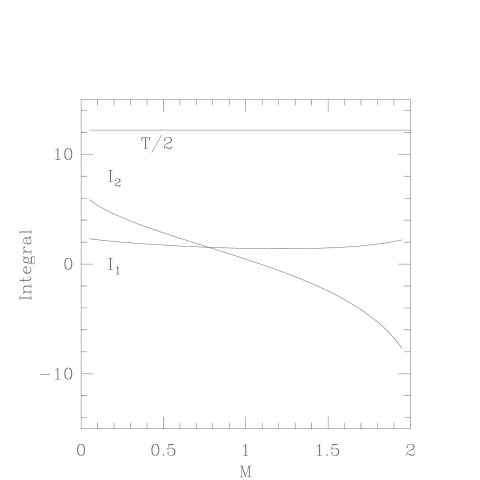
Figure 3: The three finite integrals evaluated at values of $M$, (see Eqns. (54)–(56)).

The expression for the fermion self–energy in the continuum, using dimensional regularization in the $\overline{\rm MS}$ scheme, can be written as

$$\Sigma(p,m_{f})~{}=~{}i\hbox to0.0pt{/\hss}\kern-0.8ptp\Sigma^{\overline{\rm MS}}_{1}~{}+~{}m_{f}\Sigma^{\overline{\rm MS}}_{2},$$ (59)

where $m_{f}$ is the continuum mass and

$$\Sigma_{1}^{\overline{\rm MS}} = {2}\int_{0}^{1}dx~{}x~{}\ln\Big{(}{Q^{2}\over z_{c}^{2}}\Big{)}-1,$$ (60)

$$\Sigma_{2}^{\overline{\rm MS}} = {4}\int_{0}^{1}dx~{}\ln\Big{(}{Q^{2}\over z_{c}^{2}}\Big{)}-2,$$ (61)

and $z_{c}^{2}\equiv(1-x)(p^{2}x+m_{f}^{2})$. The lattice mass and continuum mass are matched onto each other by combining these calculations so that, in Eqn. (30),

$$Z_{m}~{}=~{}{Z^{\rm LAT}_{2}\over Z^{\rm LAT}_{1}}\times{Z^{\overline{\rm MS}}_{1}\over Z^{\overline{\rm MS}}_{2}},$$ (62)

with the notation that $Z_{j}\equiv 1-g^{2}C_{F}\Sigma_{j}/16\pi^{2}$. The final mass renormalization factor between domain wall fermions and continuum fermions in the $\overline{\rm MS}$ scheme is given by

$$Z_{m}~{}=~{}1~{}-~{}{6g^{2}C_{F}\over 16\pi^{2}}\bigg{(}\ln(\mu a)-C_{m}\bigg{)},$$ (63)

where

$$C_{m}~{}=~{}\ln\pi-{1\over 4}+{1\over 6}\bigg{(}{T\over 2}+\tilde{I}_{1}-\tilde{I}_{2}\bigg{)}.$$ (64)

As discussed in detail in Sec. 3.2, the parameter $M$ is renormalized. Since the perturbative estimate of the renormalization (38) is large and untrustworthy, we use the ansatz (42). The integrals (54) and (55) are unchanged, except the trivial replacement $M\to\tilde{M}$ in Figs. 3 and 4. We mark the region of $\tilde{M}$ where our simulations have been performed with vertical dashed lines. Between those, $0.7<\tilde{M}<1.0$, $C_{m}$ varies from 2.88 to 3.10. These values of $C_{m}$ should be compared to $C_{m}=2.16$ for Wilson fermions, 3.22 for Sheikholeslami–Wohlert fermions, and 6.54 for Kogut–Susskind fermions.

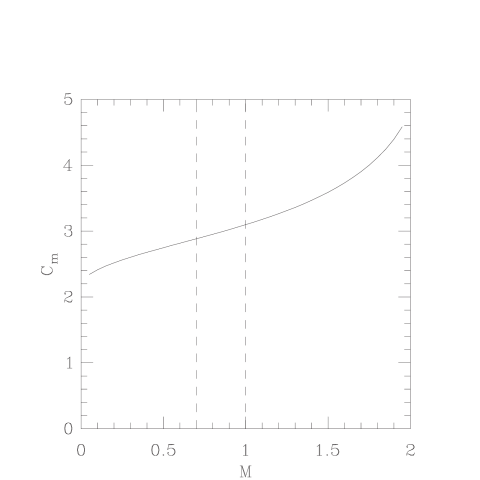
Figure 4: The matching coefficient $C_{m}$ as a function $M$. The dashed lines indicate the range of $M$ where numerical simulations have been performed.

4 Monte Carlo results

In practice, Monte Carlo simulation of quenched QCD using domain wall fermions is very similar to standard calculations using Wilson fermions. We use the conjugate gradient algorithm to invert the five–dimensional fermion matrix. Next, $4d$ quark fields are constructed from the $5d$ fields at the two boundaries [19]:

$$q(x) = P_{+}\psi_{1}(x)~{}+~{}P_{-}\psi_{N_{s}}(x)$$

$$\bar{q}(x) = \bar{\psi}_{N_{s}}(x)P_{+}~{}+~{}\bar{\psi}_{1}(x)P_{-}$$ (65)

These are the simplest interpolating fields for the lightest mode, and composite operators constructed from them satisfy exact continuum–like Ward identities in the limit $N_{s}\to\infty$ [19].

For this exploratory calculation of the strange quark mass, we compute the pseudoscalar meson mass and decay constant on a few dozen configurations at three lattice spacings. Specifically we perform Monte Carlo simulations at three values of the gauge coupling: $\beta\equiv 6/g^{2}=$ 5.85, 6.0, and 6.3. The size of the extra dimension for the main part of this work for the three couplings was $N_{s}=$ 14, 10, and 10, respectively, and the $5d$ mass parameter was $M=$ 1.7, 1.7, and 1.5, respectively. The value of $M\approx 1.7$ at 6.0 is the optimal value which suppresses propagation of the light mode in the extra dimension, as found in a previous study [24]. The $M$ at the other two $\beta$’s were ad hoc choices based on the $\beta=6.0$ value and the fact that the optimal $M$ should decrease to 1 in the weak coupling limit. At all three gauge couplings the mesonic two–point functions were computed with $m=$ 0.075 and 0.050, and at $\beta=6.0$ and 6.3 another mass, $m=0.025$, was also included. The lattice volumes at $\beta=6.0$ and 6.3 are roughly $\approx$(1.6 fm)³ while the $\beta=5.85$ volume is $\approx$(2.0 fm)³. Our raw lattice simulation results are given in Table 2.

Table 2: Pseudoscalar mass and decay constant for the main numerical data set.

	$\beta=5.85,16^{3}\times 32$		$\beta=6.0,16^{3}\times 32$		$\beta=6.3,24^{3}\times 60$
$m$	$aM_{\pi}$	$af_{\pi}$	$aM_{\pi}$	$af_{\pi}$	$aM_{\pi}$	$af_{\pi}$
0.025	–	–	0.309(6)	0.076(4)	0.245(5)	0.056(5)
0.050	0.488(5)	0.104(4)	0.423(5)	0.088(4)	0.340(4)	0.066(3)
0.075	0.588(4)	0.114(4)	0.517(5)	0.094(4)	0.425(4)	0.072(3)

In addition to the gauge coupling and bare quark mass, domain wall fermion simulations depend on the five–dimensional mass $M$ and the size of the extra dimension $N_{s}$. The study of how data are affected by changing these parameters is important. Given the results of Ref. [24], we believe that we have taken $N_{s}$ large enough so that corrections due to the mixing of the two light modes in the center of the extra dimension are smaller than the rest of our uncertainties which we will show later to be $\approx 10\%-20\%$. The effect of a finite $N_{s}$ is to give the pion an additional intrinsic mass $m_{I}$:

$$(aM_{\pi})^{2}~{}=~{}A~{}\tilde{M}~{}(2-\tilde{M})~{}(m~{}+~{}m_{I}).$$ (66)

In the free theory $m_{I}=|1-M|^{N_{s}}$ [20], and in the interacting theory $m_{I}$ is expected to decay exponentially $m_{I}\sim\exp(-\alpha N_{s})$.

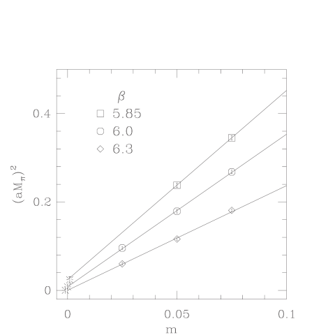
Figure 5: Lattice pseudoscalar mass vs. $m$ for the three $\beta$ values. Asterisks indicate linear extrapolations to $m=0$ with jackknifed errors and are slightly displaced horizontally for clarity.

Indeed we find a nonzero intercept when we extrapolate the pion mass squared to $m=0$ for $\beta=5.85$ and 6.0, (see Fig. 5), but find that the $\beta=6.3$ mass squared does extrapolate to zero. We have repeated simulations at $\beta=6.0$ using $N_{s}=14$ and found the pion mass decreases by a few percent (compare Tables 2 and 3) signaling a statistically significant $m_{I}$. However, errors in determining the lattice spacing from $f_{\pi}$ are much larger than the difference in $aM_{\pi}$ and so the $N_{s}=10$ results are sufficient for this work.

A thorough study of the $N_{s}$ dependence at a stronger coupling, $\beta=5.7$, was presented in Ref. [25, 26]. They find two important results. First, physical results were unchanged between $N_{s}=32$ and 48. This is consistent with arguments above concerning the behavior of domain wall fermions at stronger coupling. They used $M=1.65$ in their study. It is possible that a larger value would decrease the value of $N_{s}$ required to reach the asymptotic region. Second, even in this limit, the pion mass does not vanish as $m\to 0$, which is then presumably a ($4d$) finite volume effect.

We were able to test for finite volume errors at $\beta=6.0$ by computing the pion mass with $N_{s}=10$ on a $24^{3}\times 40$ lattice. The results, $aM_{\pi}=0.318(5)$ and 0.427(4), for $m=0.025$ and 0.050 respectively, are not statistically distinguishable from the results on the $16^{3}\times 32$ lattice (see Tab. 2).

Table 3: Pseudoscalar mass $(aM_{\pi})$ for the $\beta=6.0$, $N_{s}=14$ numerical data set.

$m$	$M=1.5$	$M=1.7$	$M=1.9$	$M=2.1$
0.025	0.290(9)	0.293(7)	0.290(7)	0.281(11)
0.050	0.394(7)	0.411(5)	0.412(7)	0.396(8)
0.075	0.487(7)	–	0.510(7)	0.490(7)

Since the quark mass, even at tree level, explicitly depends on $M$, we performed several more runs at $\beta=6.0$ with $m=0.025,0.050$ and 0.075, varying $M$ between 1.5 and 2.1 on roughly 20 configurations with $N_{s}=14$. Table 3 displays the values of $aM_{\pi}$ obtained from these simulations, and Fig. 6 shows $(aM_{\pi})^{2}$ as a function of $m$. The linear least squares fits extrapolate to $(aM_{\pi})^{2}=0$ at $m=0$ within the (uncorrelated) errors for each $M$ separately. Furthermore, in Fig. 7 we plot $(aM_{\pi})^{2}$ as a function of $M$ for the three values of $m$. We can test the ansatz (42) simply by fitting the data to

$$(aM_{\pi})^{2}=A~{}m~{}\tilde{M}~{}(2-\tilde{M}),$$ (67)

for each $m$. The dashed lines in Fig. 7 are fits to Eqn. (67) and have good $\chi^{2}$’s; each $\chi^{2}$ per degree of freedom is less than one, and $A$ is the same within (uncorrelated) errors for each $m$: $A=$ 3.48(8), 3.42(6), and 3.52(4) for $m=$ 0.025, 0.05, and 0.075, respectively. Therefore, the ansatz (42) is well justified in this work. At present the data do not permit a more general fit. Given these observations we find the definition of the lattice quark mass

$$m^{\rm LAT}~{}=~{}m~{}\tilde{M}~{}(2-\tilde{M})$$ (68)

to be very reasonable and suitable for this work.

Figure 6: Pion meson mass squared as a function of $m$ for $\beta=6.0$. Lines are least squares fits which extrapolate to $(aM_{\pi})^{2}=0$ at $m=0$ for all four values of $M$ within the errors shown by asterisks.

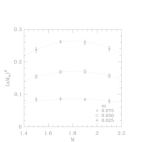
Figure 7: Pion meson mass squared as a function of $M$ at $\beta=6.0$. $N_{s}=14$ except for the $M=1.7$, $m=0.075$ point which has $N_{s}=10$. The dotted lines are fits to $(aM_{\pi})^{2}=Am\tilde{M}(2-\tilde{M})$.

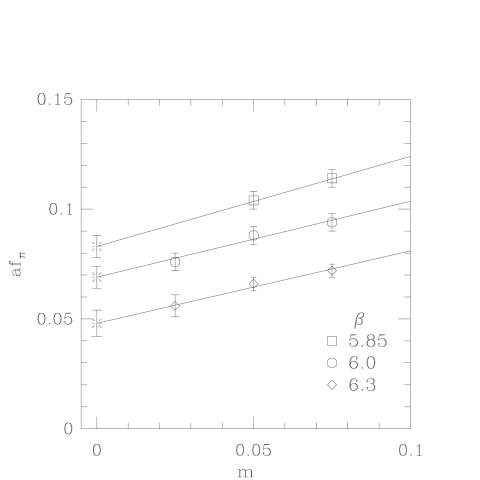
Figure 8: Lattice pseudoscalar decay constant vs. $m$ for the three $\beta$ values. Asterisks indicate linear extrapolations to $m=0$ with jackknifed errors.

5 Quark mass and coupling constant

We believe we have a good understanding of the dependence of hadron spectrum on $M$, so now we concentrate on the data at one value of $M$ per lattice spacing (as listed in Table 4). We compute the pion decay constant $af_{\pi}$ for three masses $m$ for each $\beta$ and extrapolate linearly to the chiral limit, $m=0$, (see Fig. 8). We determine the lattice spacing by setting this extrapolated value to the physical pion decay constant, $f_{\pi}=130.7$ MeV. Here we must emphasize that in this exploratory calculation, the determination of the inverse lattice spacing has a large systematic uncertainty due to having a only a few data points to extrapolate $af_{\pi}$ to $m=0$. In the continuum, $\chi$PT gives a one–loop correction to the decay constant which goes as [43]

$$f_{\pi}~{}=~{}f\bigg{[}1+{M_{\pi}^{2}\over(4\pi f)^{2}}\ln\bigg{(}{M_{\pi}^{2}\over\Lambda^{2}}\bigg{)}\bigg{]},$$ (69)

where $f$ is the tree–level decay constant and $\Lambda$ is the cutoff. With only three quark masses we cannot resolve the logarithmic behavior of $f_{\pi}$, so we extrapolate linearly to $m=0$, (see Fig. 8). We should remark that the signal for the decay constant is rather noisy: $af_{\pi}$ varies by as much as 10% depending on the range of Euclidean time over which one computes correlation functions. Since the determination of the lattice spacing for this work is through the extrapolation of $af_{\pi}$ to $m=0$, it comes with a large uncertainty.

Table 4: Summary of simulation parameters and results.

	$\beta=5.85$	$\beta=6.0$	$\beta=6.3$
# configs.	18	30	11
volume	$16^{3}\times 32$	$16^{3}\times 32$	$24^{3}\times 60$
$N_{s}$	14	10	10
$M$	1.7	1.7	1.5
$a^{-1}(f_{\pi})$ (GeV)	1.57(15)	1.89(14)	2.72(34)
$m_{s}$(MeV)	73(7)	75(6)	76(10)
$M_{c}^{W}$	0.908	0.819	0.708
$C_{m}$	2.94	3.01	2.94
$m_{s}^{\rm LAT}$(MeV)	70(7)	74(6)	73(10)
$\langle{\rm Tr}~{}U_{\rm plaq}/3\rangle$	0.5751	0.5937	0.6224
$\alpha_{V}(3.41/a)$	0.157	0.146	0.131
$Z_{m}(\mu=2{\rm GeV})$	1.30	1.34	1.34

Next, we use chiral perturbation theory as a guide to interpolate the pion mass squared linearly in the quark mass: $M_{\pi}^{2}\sim m$ to the value of $m$ which gives the physical kaon mass, 495 MeV. That value must then be doubled to take into account the fact that we use degenerate quarks in our simulations, while the physical kaon has one strange quark and one lighter non–strange quark. We denote the parameter $m$ corresponding to the physical kaon by $m_{s}$ and display our results in Table 4. Using Eqn. (68) we obtain $m_{s}^{\rm LAT}$, the domain wall strange quark mass.

Combining Eqns. (30) and (63) the following expression relates a quark mass computed on a lattice with spacing $a$ to the quark mass defined in the modified minimal subtraction scheme of dimensional regularization at momentum scale $\mu$:

$$m_{s}^{\overline{\rm MS}}(\mu)~{}=~{}m_{s}^{\rm LAT}\Bigg{[}1-{2\alpha_{s}\over\pi}\bigg{(}\ln(\mu a)-C_{m}\bigg{)}\Bigg{]},$$ (70)

where we have substituted $g^{2}/4\pi=\alpha_{s}$ and $C_{F}=4/3$. The last quantity we need is the coupling constant $\alpha_{s}$. In a one–loop calculation such as this, there is ambiguity in the definition of the coupling constant. The matching equation (70) is derived by equating the poles of the one–loop quark propagators computed in the continuum and on the lattice. Each procedure uses a differently defined coupling constant; however, the difference between the two coupling constants is a higher order correction in perturbation theory:

$$\alpha_{s}^{\rm LAT}-\alpha_{s}^{\rm CONT}~{}=~{}O(\alpha_{s}^{2}).$$ (71)

It has been known for some time that the bare coupling constant is not a good expansion parameter for lattice perturbation theory [46]. Therefore we use a physical definition related to the heavy quark potential. Specifically, we define the coupling constant using the two–loop perturbative expression for the plaquette (the $1\times 1$ Wilson loop):

$$-\ln\bigg{\langle}{1\over 3}{\rm Tr}~{}U_{\rm plaq}\bigg{\rangle}~{}=~{}{4\pi\over 3}\alpha_{V}(3.41/a)\Big{[}1~{}-~{}1.19\alpha_{V}~{}+~{}O(\alpha_{V}^{2})\Big{]}.$$ (72)

The scale $3.41/a$ has been computed by estimating and minimizing the effect of higher order terms [46]. One can run $\alpha_{V}$ to any other scale using the universal two–loop beta function. Alternatively, one can compute the continuum $\overline{\rm MS}$ coupling constant $\alpha_{\overline{\rm MS}}$ from $\alpha_{V}$ (at a scale $q$) perturbatively [47]:

$$\alpha_{\overline{\rm MS}}(qe^{-5/6})~{}=~{}\alpha_{V}(q)\Big{[}1+{2\alpha_{V}\over\pi}+O(\alpha_{V}^{2})\Big{]}.$$ (73)

Although the three–loop beta function has been computed for $\alpha_{\overline{\rm MS}}$ [48], we choose to use the two–loop beta function for consistency; the difference comes in below the 1% level.

The remaining problem is to decide on the scales and corresponding couplings to insert in the matching equation (70). Refs. [49, 50] advocate the reorganizing of lattice perturbation theory as we described above, so that the resulting expression may be “horizontally matched” to the continuum perturbative expansion. In converting our lattice quark mass into a continuum quark mass we follow the procedure described in Ref. [9]. Then the continuum matching scale $\mu$ should be set to the “best” lattice scale which minimizes the higher order corrections to the fermion self–energy. Unfortunately, it is harder to estimate $\mu$ for logarithmically divergent graphs than it was in the case of the plaquette. Therefore we resort to trying a spread of $\mu$ values. Evidence from previous work indicates that in the range $\mu=0.5/a$ to $\pi/a$ the higher order, ultraviolet–dominated, effects are minimized [46, 9]. Finally, the quark mass is run to 2 GeV using the two–loop running equation [51]. We also test the systematic error by repeating the procedure for different values of $\mu$. In Table 5 we give the strange quark masses at the matching scales, $m(\mu)$, and the mass run to $\mu=2$ GeV; we also give our values of $\alpha_{\overline{\rm MS}}$ at different scales. Our statistical errors are 3–4 times larger than the variation in $m$(2 GeV) computed with different values of $\mu$, so we cannot argue that one particular scale minimizes higher order effects in Eqn. (70).

Table 5: Strange quark masses (in MeV) in the $\overline{\rm MS}$ scheme at increasing values of the matching scale $\mu$. We give the mass at both the matching scale $\mu$ and at 2 GeV. The first pair of masses are without tadpole improvement and the second pair include tadpole improvement.

$\mu$	$\alpha_{\overline{\rm MS}}(\mu)$	$m(\mu)$	$m$(2 GeV)	$m^{\rm TI}(\mu)$	$m^{\rm TI}$(2 GeV)
$\beta=5.85$
$0.5/a$	0.275	114(11)	96(9)	108(11)	90(9)
$1/a$	0.199	96(9)	92(9)	93(9)	90(9)
$2.0$ GeV	0.181	91(9)	91(9)	90(9)	90(9)
$2/a$	0.156	85(8)	90(9)	85(8)	90(9)
$\pi/a$	0.137	81(8)	90(9)	81(8)	90(9)
$\beta=6.0$
$0.5/a$	0.243	116(9)	102(8)	111(8)	97(7)
$1/a$	0.182	99(8)	99(8)	97(7)	96(7)
$2.0$ GeV	0.178	98(8)	98(8)	96(7)	96(7)
$2/a$	0.146	89(7)	97(7)	89(7)	97(7)
$\pi/a$	0.129	85(6)	96(7)	85(7)	97(7)
$\beta=6.3$
$0.5/a$	0.202	107(14)	101(13)	103(14)	97(13)
$2.0$ GeV	0.175	99(13)	99(13)	97(13)	97(13)
$1/a$	0.159	94(12)	98(13)	93(12)	96(13)
$2/a$	0.131	86(11)	97(13)	86(11)	97(13)
$\pi/a$	0.118	82(11)	97(13)	83(11)	97(13)

One might try to improve the perturbation expansion by nonperturbatively estimating ultraviolet effects which spoil the convergence. For example, the tadpole–improvement prescription advocates perturbatively expanding the quantity $m^{\rm LAT}/u_{0}$, where $u_{0}$ is designed to be sensitive to short–distance fluctuations [46]. Therefore, the tadpole–improved quark mass, in the $\overline{\rm MS}$ scheme is related to $m^{\rm LAT}/u_{0}$ perturbatively by

$$m^{\rm TI}_{\overline{\rm MS}}(\mu)~{}=~{}\Big{(}m^{\rm LAT}\Big{/}u_{0}\Big{)}\bigg{[}1-{2\alpha_{s}\over\pi}\bigg{(}\ln\mu a~{}-~{}\Big{[}C_{m}-C_{T}\Big{]}\bigg{)}\bigg{]},$$ (74)

where $u_{0}$ is defined to be the fourth root of the plaquette

$$u_{0}~{}\equiv~{}\bigg{\langle}{1\over 3}{\rm Tr}~{}U_{\rm plaq}\bigg{\rangle}^{1/4},$$ (75)

and it is computed from Monte Carlo simulation. The matching coefficient is modified at the one loop level by the perturbative expansion of $u_{0}$

$$u_{0}~{}=~{}1-{1\over 12}g^{2}~{}\equiv~{}1-{2\over\pi}C_{T}\alpha_{s},$$ (76)

which defines $C_{T}$. In Table 5 we give the tadpole–improved strange quark mass for the various matching scales, $m^{\rm TI}(\mu)$, as well as the mass run to 2 GeV, $m^{\rm TI}$(2 GeV). At the lower scales $\mu\leq 2$ GeV, tadpole–improvement lowers the mass by 4–6 MeV indicating that the unimproved perturbative result has significant higher order corrections. On the other hand, there is no significant difference between the standard and improved expansions when the matching is done at $\mu>2$ GeV. Therefore, we will choose for our final result the improved mass with the matching done at $\mu=2/a$, $m_{\overline{\rm MS}}^{\rm TI}(2/a)$ in Table 5, and assign a 2 MeV systematic error due to the arbitrary choice of scale. We perturbatively run our final result to 2 GeV for comparison with other results.

In Figure 9 we plot our results for the strange quark mass (with statistical error bars only) in the $\overline{\rm MS}$ scheme at the scale 2 GeV along with those obtained using other fermion discretizations. In choosing the data to which we compare the domain wall results, we used those which were obtained with the same method. The masses were computed by fixing the kaon to be its physical mass and the matchings to the continuum were computed perturbatively. Unfortunately, we can only set the lattice spacing using $f_{\pi}$ while the other data in Fig. 9 use the $\rho$ meson mass. In typical Wilson fermion simulations [52], as well as preliminary domain wall fermion simulations [53], there is a $\approx 15\%$ systematic uncertainty due to choosing $f_{\pi}$ vs. $M_{\rho}$ to set the scale.

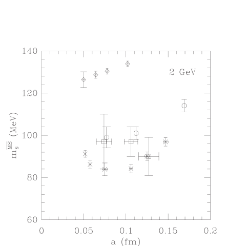
Figure 9: Strange quark mass in $\overline{\rm MS}$ scheme at 2 GeV. Our results are displayed as squares, Wilson fermions as diamonds [14], Sheikholeslami–Wohlert fermions as circles [8], and Kogut–Susskind results as crosses [44, 45].

In this first work, the statistical errors are rather large, about 15%, yet it is encouraging that we see no significant signs of scaling violations. As argued in Sec. 2.3, discretization errors should be $O(a^{2})$ rather than $O(a)$ since wrong–chirality operators are suppressed; however, a more precise study is needed to draw a firm conclusion. Since no scale dependence can be detected within the statistical errors in this exploratory study, we take a weighted average of the strange quark mass determined at the three lattice spacings to give 95 MeV with a purely statistical uncertainty of 5 MeV. A linear extrapolation to the continuum limit raises the central value by 15 MeV, but of course has a large uncertainty. Given that we do not expect to have $O(a)$ scaling violations, we take 95 MeV as our strange quark mass but add the 15 MeV in quadrature with the rest of our systematic errors.

The largest systematic error arises from the ambiguity in which physical quantity is used to fix the lattice spacing. As mentioned above, preliminary results and experience with Wilson fermions lead us to believe there could be at least a 15% uncertainty using domain wall fermions. Considering that our calculation of $f_{\pi}$ was done with only a few quark masses, we conservatively estimate a 20% systematic uncertainty in $a^{-1}$; the other systematic errors are small in comparison. For example, the uncertainty in matching scale induces an error of 2 MeV. We have not yet computed the strange quark mass by fixing the $\phi$ meson to its physical mass, but in Wilson fermion simulations there is an $O(10\%)$ difference from the strange quark mass using the kaon. For now we include this error as a systematic uncertainty in our calculation, but it must be explicitly checked with domain wall fermions. Of course quenching also induces a systematic error; however, we are unable to address its effects without a full dynamical–fermion simulation.

Table 6: Sources of systematic uncertainty in computing the strange quark mass.

Source	Estimated size
Using $f_{\pi}$ vs. $M_{\rho}$ to set $a$	20%
Matching scale, $\mu$	2%
Using $\phi$ vs. $K$ to set $m_{s}$	10%
Continuum extrapolation	16%

Adding the statistical and systematic errors in quadrature, our final result for the strange quark mass within the quenched approximation is

$$m_{\overline{\rm MS}}(2~{}{\rm GeV})~{}=~{}95(26)~{}{\rm MeV}.$$ (77)

6 Conclusions

This work has focused on the steps needed to compute the light quark masses with the domain wall fermion discretization. We have extended the calculation of the domain wall fermion self–energy to the massive case. We find that the perturbative mass renormalization factor which matches the domain wall lattice regularization to the $\overline{\rm MS}$ regularization scheme is as well–behaved as that for Wilson fermions.

In conjunction with the perturbative calculation, we have performed numerical simulations of quenched lattice QCD using domain wall fermions. At $\beta=6.0$ the pion mass squared vanishes linearly in $m$ as $m\rightarrow 0$, and the ansatz $M\to M-M_{c}^{W}$ is a good fit to the data. Finally we compute the strange quark mass $m_{\overline{\rm MS}}$(2 GeV) at three lattice spacings. Within our errors, the results are scale independent so we take a weighted average giving $m_{\overline{\rm MS}}(2~{}{\rm GeV})~{}=~{}95(26)$ MeV, where systematic uncertainties (except for quenching effects) have been added in quadrature with the statistical error.

We intend to perform a larger scale calculation which will include the vector meson spectrum. This will allow us to calculate the “average” light quark mass $(m_{u}+m_{d})/2$ together with the strange quark mass. In addition we will be able to estimate the systematic error due to setting the lattice scale from $f_{\pi}$ vs. $M_{\rho}$. A higher statistics study will be able to sensitively test for scaling violations, and possibly give a value for the light quark masses which is comparable in precision to other lattice calculations.

Future prospects for this formulation are promising. Domain wall fermions have an advantage over Wilson fermions, improved or not, in that they have chiral symmetry which is broken only by the explicit mass $m$ coupling the boundaries – the mixing of the two modes in between the boundaries can be made negligible compared to $m$. Consequently there is no mixing between operators of different chirality and the quark mass is protected from additive renormalization. A lattice discretization which respects the axial symmetries of continuum QCD has an excellent chance to improve calculations of matrix elements involving light hadrons.

Appendix A Diagonalization

A.1 Tree level

In this Appendix we discuss the spectrum of the domain wall Dirac operator at zero momentum at tree level. Although this work appears in Ref. [18], a treatment here is useful to establish our notation, which is similar to Ref. [21].

Given the mass matrix $\Omega_{0}$, defined in Eqn. (11), we wish to solve the eigenvalue equation

$$\Big{(}\Omega_{0}\Omega_{0}^{\dagger}\Big{)}_{s,s^{\prime}}\phi^{(i)}_{s^{\prime}}~{}=~{}(\lambda_{0}^{(i)})^{2}\phi^{(i)}_{s},$$ (78)

where the index $i\in[1,N_{s}]$ labels the eigenstates. The general equation to be satisfied is

$$\Big{(}1+b_{0}^{2}-\lambda_{0}^{2}\Big{)}\phi_{s}-b_{0}\Big{(}\phi_{s+1}+\phi_{s-1}\Big{)}~{}=~{}0.$$ (79)

If $0<b_{0}<1$ then the general solutions are of the form

$$\phi_{s}~{}=~{}Ae^{\alpha_{0}s}+Be^{-\alpha_{0}s}$$ (80)

where $\alpha_{0}$ is defined through

$$\cosh\alpha_{0}~{}=~{}{1+b_{0}^{2}-(\lambda_{0}^{(i)})^{2}\over 2|b_{0}|}.$$ (81)

If $-1<b_{0}<0$ then the general solutions are of the form

$$\phi_{s}~{}=~{}(-1)^{s}\Big{(}Ae^{\alpha_{0}s}+Be^{-\alpha_{0}s}\Big{)}.$$ (82)

For $(\lambda_{0}^{(i)})^{2}<(1-b_{0})^{2}$ or $(\lambda_{0}^{(i)})^{2}>(1+b_{0})^{2}$, $\alpha$ becomes imaginary and

$$\cos i\alpha_{0}~{}=~{}{1+b_{0}^{2}-(\lambda_{0}^{(i)})^{2}\over 2b_{0}}.$$ (83)

Let us concentrate on the first case of exponential damping. We must apply the boundary conditions

$$\Big{(}b_{0}^{2}+a^{2}m^{2}-(\lambda_{0}^{(1)})^{2}\Big{)}\phi_{1}-b_{0}~{}\phi_{2}+am~{}b_{0}~{}\phi_{N_{s}} = 0$$ (84)

$$\Big{(}1+b_{0}^{2}-(\lambda_{0}^{(1)})^{2}\Big{)}\phi_{N_{s}}-b_{0}~{}\phi_{N_{s}-1}+am~{}b_{0}~{}\phi_{1} = 0.$$ (85)

In order to make these conditions consistent with the general equation (79), $\phi_{s=0}$ and $\phi_{s=N_{s}+1}$ must satisfy

$$-b_{0}~{}\phi_{0}~{}+~{}\phi_{1} = (am)^{2}~{}\phi_{1}-am~{}b_{0}~{}\phi_{N_{s}}$$ (86)

$$-b_{0}~{}\phi_{N_{s}+1} = am~{}b_{0}~{}\phi_{1}.$$ (87)

As has been found previously [18, 21, 20], the eigenvalue is

$$(\lambda^{(1)})^{2} = (am)^{2}(1-b_{0}^{2})^{2}~{}+~{}O\Big{(}(am)^{4}\Big{)}~{}+~{}O\Big{(}b_{0}^{N_{s}}\Big{)}$$ (88)

$$= (am)^{2}M^{2}(2-M)^{2}~{}+~{}O\Big{(}(am)^{4}\Big{)}~{}+~{}O\Big{(}(1-M)^{N_{s}}\Big{)}.$$

The corresponding normalized eigenvector is

$$\phi_{s}^{(1)} = \sqrt{1-b_{0}^{2}}~{}e^{-\alpha_{0}(s-1)}$$ (89)

$$= \sqrt{M(2-M)}~{}e^{-\alpha_{0}(s-1)}.$$

The eigenvectors corresponding to the heavier modes can be decomposed into a basis of sine functions

$$\phi_{s}^{(i)}~{}=~{}\sqrt{{2\over N_{s}}}~{}\sin\bigg{(}{\pi(i-1)\over N_{s}}\Big{[}N_{s}+1-s\Big{]}\bigg{)};\hskip 8.5359pt{\rm for}~{}i\neq 1$$ (90)

Note that if $b_{0}<0$ then

$$\phi_{s}^{(1)}~{}=~{}(-1)^{s}\sqrt{1-b_{0}^{2}}~{}e^{-\alpha_{0}(s-1)}$$ (91)

while the other eigenvectors and all the eigenvalues are unchanged. Also, the eigenvalues and eigenvectors are the same for $\Omega_{0}^{\dagger}\Omega_{0}$ with the substitution $s\rightarrow N_{s}+1-s$. Let us define unitary matrices which diagonalize $\Omega_{0}\Omega_{0}^{\dagger}$ as

$$U^{(0)}_{s,s^{\prime}}~{}\equiv\phi^{(s)}_{s^{\prime}}$$ (92)

and which diagonalize $\Omega_{0}^{\dagger}\Omega_{0}$ as

$$V^{(0)}_{s,s^{\prime}}~{}\equiv\phi^{(s)}_{N_{s}+1-s^{\prime}}.$$ (93)

A.2 One–loop level

As in Appendix A.1, we want to derive an effective action for the lightest eigenstate. In general this involves computing one–loop corrections to the matrices $U$ and $V$ which diagonalize the square of the mass matrix, $\Omega$. However, it has already been shown [21, 22] that the light mode is stable under radiative corrections. Following Ref. [21], let us write the mass matrix as

$$\Omega~{}=~{}W^{-}~{}+~{}g^{2}\Omega_{1}~{}\equiv~{}W^{-}~{}+~{}{g^{2}C_{F}\over 16\pi^{2}}\Big{(}\Sigma^{(0),-}~{}+~{}am\Sigma^{(2),-}\Big{)},$$ (94)

where the $\Sigma^{(j)}$ are given in Eqns. (32) – (34) and $\Sigma^{(j),\pm}\equiv\Sigma^{(j)}P_{\pm}$. Then, to diagonalize $\Omega\Omega^{\dagger}$ to $O(g^{2})$, one must compute the corrections to $U$ and $V$:

$$U^{(0)} \rightarrow U\equiv(1+g^{2}U^{(1)})U^{(0)}$$

$$V^{(0)} \rightarrow V\equiv(1+g^{2}V^{(1)})V^{(0)},$$ (95)

If we write the one–loop eigenvalue equations as

$$\Big{(}U\Omega\Omega^{\dagger}U^{\dagger}\Big{)}_{s,s^{\prime}}~{}=~{}\Big{[}(\lambda_{0}^{(s)})^{2}+g^{2}(\lambda_{1}^{(s)})^{2}\Big{]}\delta_{s,s^{\prime}},$$ (96)

and

$$\Big{(}V\Omega^{\dagger}\Omega V^{\dagger}\Big{)}_{s,s^{\prime}}~{}=~{}\Big{[}(\lambda_{0}^{(s)})^{2}+g^{2}(\lambda_{1}^{(s)})^{2}\Big{]}\delta_{s,s^{\prime}},$$ (97)

then it can be shown that [21]

$$U^{(1)}_{s,s^{\prime}} = \bigg{[}\lambda_{0}^{(s)}(U^{(0)}\Omega_{1}V^{(0)}{}^{\dagger})_{s,s^{\prime}}+\lambda_{0}^{(s^{\prime})}(U^{(0)}\Omega_{1}V^{(0)}{}^{\dagger})_{s^{\prime},s}\bigg{]}\bigg{/}\bigg{[}(\lambda_{0}^{(s)})^{2}-(\lambda_{0}^{(s^{\prime})})^{2}\bigg{]}$$

$$V^{(1)}_{s,s^{\prime}} = \bigg{[}(U^{(0)}\Omega_{1}V^{(0)}{}^{\dagger})_{s,s^{\prime}}\lambda_{0}^{(s^{\prime})}+(U^{(0)}\Omega_{1}V^{(0)}{}^{\dagger})_{s^{\prime},s}\lambda_{0}^{(s)}\bigg{]}\bigg{/}\bigg{[}(\lambda_{0}^{(s)})^{2}-(\lambda_{0}^{(s^{\prime})})^{2}\bigg{]}$$

for $s\neq s^{\prime}$, and

$$U^{(1)}_{s,s}~{}=~{}V^{(1)}_{s,s}~{}=~{}0,$$ (98)

and, most importantly,

$$(\lambda_{1}^{(s)})^{2}~{}=~{}2(U^{(0)}\Omega_{1}V^{(0)}{}^{\dagger})_{s,s}\lambda_{0}^{(s)}.$$ (99)

Therefore, in order to compute the quark mass to one loop, we need $(U^{(0)}\Omega_{1}V^{(0)}{}^{\dagger})_{1,1}$. Aoki and Taniguchi [21] have shown that $U^{(0)}\Sigma_{0,-}V^{(0)}{}^{\dagger}$ is negligibly small, and in Appendix B we compute $U^{(0)}\Sigma^{(2),-}V^{(0)}{}^{\dagger}\Big{|}_{1,1}$ and $V^{(0)}\Sigma^{(2),+}U^{(0)}{}^{\dagger}\Big{|}_{1,1}$.

Appendix B Perturbative calculation – details

B.1 Feynman rules

The Feynman rules are similar to those for Wilson fermions plus plaquette–action gluons [54].

In the gauge sector, we use the usual four dimensional plaquette action:

$$S_{g}~{}=~{}\beta\sum_{\rm plaq}{1\over 3}~{}{\rm Re~{}Tr~{}}(1-U_{\rm plaq}).$$ (100)

In the five dimensional picture there are simply $N_{s}$ copies of the gauge field, and in the flavor interpretation the gluons are simply flavorless.

The propagator of a gluon (in Feynman gauge) with momentum $q$ is given by

$$D_{\mu\nu}(q)~{}=~{}{\delta_{\mu\nu}\over 4\sum_{\rho}\sin^{2}(aq_{\rho}/2)}~{}\equiv~{}{\delta_{\mu\nu}\over\hat{q}^{2}}.$$ (101)

The one-gluon – fermion vertex with incoming (outgoing) momentum $p_{1}$ ($p_{2}$) is $gt_{n}v_{\mu}(q)$, where

$$v_{\mu}(q)~{}=~{}\Big{(}i\gamma_{\mu}\cos aq_{\mu}-\sin aq_{\mu}\Big{)},$$ (102)

$q=(p_{1}+p_{2})/2$, and $t_{n}$ is one of the eight generators of $SU(3)$. The two-gluon – fermion vertex with gluon indices $n,\mu$ and $n,\mu^{\prime}$ and fermion momenta as above is $(g^{2}/2)\{t_{n},t_{n^{\prime}}\}\delta_{\mu,\mu^{\prime}}$, with

$$w_{\mu}(q)~{}=~{}-\Big{(}i\gamma_{\mu}\sin aq_{\mu}+\cos aq_{\mu}\Big{)}.$$ (103)

The massive fermion propagator for the boundary wall variant used in this work was derived in Ref. [18] and also Ref. [21] whose notation we adopt. The tree–level $G^{R}$ and $G^{L}$, as defined in Eqn. (20), are given by

$$G^{R}_{s,s^{\prime}}~{}=~{}G^{0}_{s,s^{\prime}}+A_{++}e^{\alpha(s+s^{\prime})}+2A_{+-}\cosh\alpha(s-s^{\prime})+A_{--}e^{-\alpha(s+s^{\prime})}$$ (104)

and

$$G^{L}_{s,s^{\prime}}~{}=~{}G^{0}_{s,s^{\prime}}+B_{++}e^{\alpha(s+s^{\prime})}+2B_{+-}\cosh\alpha(s-s^{\prime})+B_{--}e^{-\alpha(s+s^{\prime})}.$$ (105)

The inhomogeneous part of the solution is

$$G^{0}_{s,s^{\prime}}~{}=~{}A\cosh\Big{(}\alpha(N_{s}-|s-s^{\prime}|)\Big{)},$$ (106)

and the constants defined implicitly above are

$$A = {1\over 4b\sinh\alpha~{}\sinh(\alpha N_{s})}$$ (107)

$$A_{++} = (e^{-2\alpha N_{s}}-1)(1-be^{e}{-\alpha})(1-m^{2})A/F$$ (108)

$$A_{+-} = 2b\sinh\alpha(1+2m\cosh(\alpha N_{s})+m^{2})A/F$$ (109)

$$A_{--} = (1-e^{2\alpha N_{s}})(1-be^{\alpha})(1-m^{2})A/F$$ (110)

$$B_{++} = (e^{-2\alpha N_{s}}-1)e^{-\alpha}(e^{-\alpha}-b)(1-m^{2})A/F$$ (111)

$$B_{+-} = 2b\sinh\alpha(1+2m\cosh(\alpha N_{s})+m^{2})A/F$$ (112)

$$B_{--} = (1-e^{2\alpha N_{s}})e^{\alpha}(e^{\alpha}-b)(1-m^{2})A/F$$ (113)

where

$$F=e^{\alpha N_{s}}\Big{[}1-be^{\alpha}+m^{2}(be^{-\alpha}-1)\Big{]}-4bm\sinh\alpha+e^{-\alpha N_{s}}\Big{[}be^{-\alpha}-1+m^{2}(1-be^{\alpha})\Big{]}.$$ (114)

B.2 Tadpole diagram

The tadpole diagram (Fig. 1a) is simple to compute. Since it has no fermion propagator in the loop, it is equivalent to the case for Wilson fermions:

$$\Sigma^{\rm tad}_{s,s^{\prime}}(p) = {16\pi^{2}\delta_{s,s^{\prime}}\over a}\sum_{\mu}\int_{-\pi}^{\pi}{d^{4}l\over(2\pi)^{4}}w_{\mu}(ap)D_{\mu\nu}(l)$$ (115)

$$= -{\delta_{s,s^{\prime}}\over 2}\Big{(}i\hbox to0.0pt{/\hss}\kern-0.8ptp+{4\over a}\Big{)}T,$$

where $T$ is the finite integral

$$T~{}=~{}16\pi^{2}\int_{-\pi}^{\pi}{d^{4}l\over(2\pi)^{4}}{1\over 4\sum_{\mu}\sin^{2}(l_{\mu}/2)}~{}=~{}24.4.$$ (116)

B.3 Taylor expansion

The calculation of the half–circle graph (Fig. 1b) with domain wall fermions parallels the same calculation with Wilson fermions [35]. The contribution of the half–circle graph to the fermion self–energy is

$$\Sigma^{\rm h-c}_{s,s^{\prime}}(p,m) = {16\pi^{2}\over a}\int_{-\pi}^{\pi}{d^{4}l\over(2\pi)^{4}}\sum_{\mu,\nu}v_{\mu}\Big{(}{l+ap\over 2}\Big{)}S^{F}_{s,s^{\prime}}(l,am)D_{\mu\nu}(ap-l)v_{\nu}\Big{(}{l+ap\over 2}\Big{)}.$$ (117)

$$\equiv {16\pi^{2}\over a}\int_{-\pi}^{\pi}{d^{4}l\over(2\pi)^{4}}E(l,ap,am).$$ (118)

The second line above defines the integrand $E$.

A simple Taylor expansion of Eqn. (117) about zero lattice spacing would not be valid due to the logarithmic divergence of the integral. That is, the coefficients of the power series in $a$ would have a $\ln a$ dependence, which must first be separated before expanding the Taylor series. We subtract and then add back a similar half–circle graph built from continuum–like Feynman rules designed to have the same infrared behavior as the present rules.

$$\Sigma^{\rm IR}_{s,s^{\prime}}(p,m) = {16\pi^{2}\over a}\int_{-\pi}^{\pi}{d^{4}l\over(2\pi)^{4}}~{}\Theta(\pi^{2}-l^{2})~{}{(i\gamma_{\mu})~{}S^{\rm IR}_{s,s^{\prime}}(l,am)~{}(i\gamma_{\mu})\over(ap-l)^{2}}$$ (119)

$$\equiv {16\pi^{2}\over a}\int_{-\pi}^{\pi}{d^{4}l\over(2\pi)^{4}}E^{\rm IR}(l,ap,am).$$ (120)

The step function $\Theta(\pi^{2}-l^{2})$ makes the integral spherically symmetric and therefore easier to evaluate. We will specify the continuum–like fermion propagator $S^{\rm IR}$ in the next Section.

Now we can write the half-circle graph in terms of a Taylor expansion of $(\Sigma-\Sigma^{\rm IR})$

$$\Sigma^{\rm h-c}(p,m) = {16\pi^{2}\over a}\int_{l}~{}\Theta(\pi^{2}-l^{2})E^{\rm IR}(l,ap,am)$$ (121)

$$+ {1\over a}\int_{l}\Big{[}E(l,ap,am)-\Theta(\pi^{2}-l^{2})E^{\rm IR}(l,ap,am)\Big{]}$$

$$= {16\pi^{2}\over a}\int_{l}~{}\Theta(\pi^{2}-l^{2})\Big{[}E^{\rm IR}(l,ap,am)-E^{\rm IR}(l,0,0)\Big{]}+{1\over a}\int_{l}E(l,0,0)$$

$$+ \int_{l}{d\over da}\Big{[}E(l,ap,am)-\Theta(\pi^{2}-l^{2})E^{\rm IR}(l,ap,am)\Big{]}\Big{|}_{a=0}~{}+~{}O(a).$$

We use a shorthand notation for the loop integral, namely $\int_{l}\equiv\int d^{4}l/(2\pi)^{4}$. Eqn. (121) is the “master” equation for computing the half–circle graph: in the remainder of this Appendix, we compute the various terms appearing within it.

B.4 Infrared terms

In this Section, we compute $E^{\rm IR}$ and $dE^{\rm IR}/da$. The IR ($a\to 0$) limit of the fermion propagator is

$$S^{\rm IR}(l,am)~{}=~{}{1\over l^{2}+a^{2}(m_{q}^{(0)})^{2}}\sum_{+,-}(-i\hbox to0.0pt{/\hss}\kern 0.0ptl-am\delta_{\pm}+\Delta_{\pm})C_{\pm}P_{\pm},$$ (122)

where $\delta_{+}=\delta_{s,1}\delta_{s^{\prime},N_{s}}$, $\delta_{-}=\delta_{s,N_{s}}\delta_{s^{\prime},1}$, $\Delta_{\pm}=\delta_{s\mp 1,s^{\prime}}-b_{0}\delta_{s,s^{\prime}}$, and

$$C_{+} = (1-b_{0}^{2})b_{0}^{2N_{s}-s-s^{\prime}}+am_{q}^{(0)}b_{0}^{N_{s}}\Big{(}b_{0}^{s-s^{\prime}}+b_{0}^{-s+s^{\prime}}\Big{)}$$ (123)

$$C_{-} = (1-b_{0}^{2})b_{0}^{s+s^{\prime}-2}+am_{q}^{(0)}b_{0}^{N_{s}}\Big{(}b_{0}^{s-s^{\prime}}+b_{0}^{-s+s^{\prime}}\Big{)}.$$ (124)

Note also the presence of the tree–level quark mass $m_{q}^{(0)}=mM(2-M)$ which was defined above in Eqn. (26).

Let us first compute the integral of $dE^{\rm IR}/da$. Since the IR vertices are just $i\gamma_{\mu}$, there will be just two terms, one with $dS^{\rm IR}(l,am)/da$ and the other with $d(ap-l)^{-2}/da$. The result for the first term is

$$\int_{l}\Theta\sum_{\mu}{(i\gamma_{\mu})S^{\rm IR}(l,am)(-2p)\cdot(ap-l)(i\gamma_{\mu})\over(ap-l)^{4}}\bigg{|}_{a=0}~{}=~{}\int_{l}\Theta\sum_{+,-}{-i\hbox to0.0pt{/\hss}\kern-0.8ptpC^{0}_{\mp}P_{\pm}\over l^{4}},$$ (125)

where $C^{0}\equiv C|_{a=0}$, and $\Theta=\Theta(\pi^{2}-l^{2})$. Note the $\Delta_{\pm}$ term in the fermion propagator is anti-symmetric in $l$ and so vanishes upon integration above. The second term comes from taking the derivative of $S^{\rm IR}$:

$${d\over da}S^{\rm IR}(l,am)\Big{|}_{a=0} = -S^{\rm IR}(l,0)\bigg{[}{d\over da}\Big{(}S^{\rm IR}(l,am)\Big{)}^{-1}\bigg{]}\bigg{|}_{a=0}S^{\rm IR}(l,0)$$ (126)

$$= \sum_{+,-}{m\over l^{4}}\bigg{[}(-i\hbox to0.0pt{/\hss}\kern 0.0ptl+\Delta_{\pm})~{}C^{0}_{\pm}P_{\pm}\delta_{\pm}~{}(-i\hbox to0.0pt{/\hss}\kern 0.0ptlC^{0}_{\pm}+\Delta_{\pm}C^{0}_{\mp})P_{\pm}\bigg{]}$$

After some algebra, we have

$$\int_{l}{1\over l^{2}}\bigg{[}(i\gamma_{\mu}){d\over da}S^{\rm IR}(i\gamma_{\mu})\bigg{]}_{s,s^{\prime}}\bigg{|}_{a=0} = -4(16\pi^{2})m_{q}^{(0)}\int_{l}\Theta{1-b_{0}^{2}\over l^{4}}\Big{[}b_{0}^{N_{s}-s+s^{\prime}-1}P_{+}$$ (127)

$$-b_{0}^{N_{s}+s-s^{\prime}-1}P_{-}\Big{]}.$$

The integration of the $E^{\rm IR}(l,ap,am)-E^{\rm IR}(l,0,0)$ term of Eqn. (121) is quite similar to that for Wilson fermions (see e.g. [35]). We delay writing down the answer, since it simplifies greatly upon diagonalization in flavor space.

B.5 Finite terms

Let’s first look at the numerator of $E(l,ap,am)$. For the time being we suppress the indices $s,s^{\prime}$.

$${\cal N} \equiv \sum_{\mu}v_{\mu}((l+ap)/2)S^{F}(l,am)v_{\mu}((l+ap)/2)$$ (128)

$$= \sum_{\mu}\Big{[}i\gamma_{\mu}\cos{1\over 2}(l+ap)_{\mu}-\sin{1\over 2}(l+ap)_{\mu}\Big{]}\Big{[}(-i\bar{\hbox to0.0pt{/\hss}\kern 0.0ptl}+W^{-})G^{R}P_{+}+(-i\bar{\hbox to0.0pt{/\hss}\kern 0.0ptl}+W^{+})G^{L}P_{-}\Big{]}$$

$$\times \Big{[}i\gamma_{\mu}\cos{1\over 2}(l+ap)_{\mu}-\sin{1\over 2}(l+ap)_{\mu}\Big{]}$$

Multiplying the factors of ${\cal N}$ gives

$${\cal N}= - \sum_{\mu}\Big{(}-i\gamma_{\mu}~{}\bar{\hbox to0.0pt{/\hss}\kern 0.0ptl}~{}\gamma_{\mu}~{}+~{}W^{-}\Big{)}~{}G^{R}P_{-}~{}\Big{(}\cos^{2}{1\over 2}(l+ap)_{\mu}\Big{)}$$ (129)

$$- \sum_{\mu}\Big{(}-i\gamma_{\mu}~{}\bar{\hbox to0.0pt{/\hss}\kern 0.0ptl}~{}\gamma_{\mu}~{}+~{}W^{+}\Big{)}~{}G^{L}P_{+}~{}\Big{(}\cos^{2}{1\over 2}(l+ap)_{\mu}\Big{)}$$

$$+ \Big{(}-i\bar{\hbox to0.0pt{/\hss}\kern 0.0ptl}~{}+~{}W^{-}\Big{)}~{}G^{R}P_{+}~{}\Big{(}\sum_{\mu}\sin^{2}{1\over 2}(l+ap)_{\mu}\Big{)}$$

$$+ \Big{(}-i\bar{\hbox to0.0pt{/\hss}\kern 0.0ptl}~{}+~{}W^{+}\Big{)}~{}G^{L}P_{-}~{}\Big{(}\sum_{\mu}\sin^{2}{1\over 2}(l+ap)_{\mu}\Big{)}$$

$$- \sum_{\mu}i\gamma_{\mu}\Big{(}-i\bar{\hbox to0.0pt{/\hss}\kern 0.0ptl}~{}+~{}W^{-}\Big{)}~{}G^{R}P_{+}~{}\Big{(}{1\over 2}\sin(l+ap)_{\mu}\Big{)}$$

$$- \sum_{\mu}\Big{(}-i\bar{\hbox to0.0pt{/\hss}\kern 0.0ptl}~{}+~{}W^{-}\Big{)}i\gamma_{\mu}~{}G^{R}P_{-}~{}\Big{(}{1\over 2}\sin(l+ap)_{\mu}\Big{)}$$

$$- \sum_{\mu}i\gamma_{\mu}\Big{(}-i\bar{\hbox to0.0pt{/\hss}\kern 0.0ptl}~{}+~{}W^{+}\Big{)}~{}G^{L}P_{-}~{}\Big{(}{1\over 2}\sin(l+ap)_{\mu}\Big{)}$$

$$- \sum_{\mu}\Big{(}-i\bar{\hbox to0.0pt{/\hss}\kern 0.0ptl}~{}+~{}W^{+}\Big{)}i\gamma_{\mu}~{}G^{L}P_{+}~{}\Big{(}{1\over 2}\sin(l+ap)_{\mu}\Big{)},$$

where, as usual, $\bar{\hbox to0.0pt{/\hss}\kern 0.0ptl}\equiv\sum_{\nu}\gamma_{\nu}\bar{l}_{\nu}$. To compute $\int_{l}E(l,0,0)$ we divide Eqn. (129) by $\hat{l}^{2}$ and integrate. Since the integration region is symmetric in $l_{\mu}$, the terms odd in $l_{\mu}$ in (129) vanish upon integration. The result is given by

$$\int_{l}E(l,0,0) = \int_{l}~{}{1\over\hat{l}^{2}}\bigg{\{}\sum_{\mu}\sin^{2}{l_{\mu}\over 2}\Big{[}(W_{0}^{-}G^{R})_{s,s^{\prime}}P_{+}+(W_{0}^{+}G^{L})_{s,s^{\prime}}P_{-}\Big{]}$$ (130)

$$- \sum_{\mu}\cos^{2}{l_{\mu}\over 2}\Big{[}(W_{0}^{+}G^{L})_{s,s^{\prime}}P_{+}+(W_{0}^{-}G^{R})_{s,s^{\prime}}P_{-}\Big{]}-{\bar{l}^{2}\over 2}\Big{(}G^{R}_{s,s^{\prime}}+G^{L}_{s,s^{\prime}}\Big{)}\bigg{\}}$$

where $W_{0}^{\pm}\equiv W^{\pm}|_{am=0}$.

Next we compute

$${d\over da}E(l,ap,am)\bigg{|}_{a=0}~{}\equiv~{}i\hbox to0.0pt{/\hss}\kern-0.8ptp{\cal E}^{1}~{}+~{}m{\cal E}^{2},$$ (131)

where

$$i\hbox to0.0pt{/\hss}\kern-0.8ptp{\cal E}^{1} = \sum_{\mu}2v_{\mu}((l+ap)/2)S^{F}(l,am){d\over da}\bigg{(}v_{\mu}((l+ap)/2)\bigg{)}\widehat{(l-ap)}^{-2}$$

$$+~{}{\cal N}{d\over da}\bigg{(}\widehat{(l-ap)}^{-2}\bigg{)}$$

$${\rm and}~{}~{}m{\cal E}^{2} = v_{\mu}((l+ap)/2)~{}{dS^{F}\over da}~{}v_{\mu}((l+ap)/2)~{}\widehat{(l-ap)}^{-2}.$$ (132)

Note that $v_{\mu}S^{F}(dv_{\mu}/da)$ is the same as Eqn. (129) with the replacements

$$\cos^{2}{1\over 2}(l+ap)_{\mu} \rightarrow -{p_{\mu}\over 2}\sin(l+ap)_{\mu}$$

$$\sin^{2}{1\over 2}(l+ap)_{\mu} \rightarrow {p_{\mu}\over 2}\sin(l+ap)_{\mu}$$ (133)

$${1\over 2}\sin(l+ap)_{\mu} \rightarrow {p_{\mu}\over 2}\cos(l+ap)_{\mu}.$$

After some algebra, the result is ${\cal E}^{1}_{s,s^{\prime}}={\cal E}^{1,+}_{s,s^{\prime}}P_{+}+{\cal E}^{1,-}_{s,s^{\prime}}P_{-}$, where

$$\int_{l}{\cal E}^{1,+}_{s,s^{\prime}} = -\int_{l}\bigg{\{}{1\over 8\hat{l}^{2}}\bigg{[}\bar{l}^{2}\Big{(}G^{R}_{s,s^{\prime}}+G^{L}_{s,s^{\prime}}\Big{)}+\sum_{\mu}\cos l_{\mu}\Big{(}(W_{0}^{-}G^{R})_{s,s^{\prime}}+(W_{0}^{+}G^{L})_{s,s^{\prime}}\Big{)}\bigg{]}$$ (134)

$$+ {1\over 2\hat{l}^{4}}\bigg{[}\bar{l}^{2}\Big{(}\sum_{\mu}\sin^{2}{l\mu\over 2}\Big{)}G^{R}_{s,s^{\prime}}-\sum_{\mu}\bar{l}^{2}_{\mu}\Big{(}2\cos^{2}{l_{\mu}\over 2}-\sum_{\nu}\cos^{2}{l_{\nu}\over 2}\Big{)}G^{L}_{s,s^{\prime}}$$

$$+ {\bar{l}^{2}\over 2}\Big{(}(W_{0}^{-}G^{R})_{s,s^{\prime}}+(W_{0}^{+}G^{L})_{s,s^{\prime}}\Big{)}\bigg{]}\bigg{\}}$$

and

$$\int_{l}{\cal E}^{1,-}_{s,s^{\prime}} = -\int_{l}\bigg{\{}{1\over 8\hat{l}^{2}}\bigg{[}\bar{l}^{2}\Big{(}G^{R}_{s,s^{\prime}}+G^{L}_{s,s^{\prime}}\Big{)}+\sum_{\mu}\cos l_{\mu}\Big{(}(W_{0}^{-}G^{R})_{s,s^{\prime}}+(W_{0}^{+}G^{L})_{s,s^{\prime}}\Big{)}\bigg{]}$$ (135)

$$+ {1\over 2\hat{l}^{4}}\bigg{[}\bar{l}^{2}\Big{(}\sum_{\mu}\sin^{2}{l\mu\over 2}\Big{)}G^{L}_{s,s^{\prime}}-\sum_{\mu}\bar{l}^{2}_{\mu}\Big{(}2\cos^{2}{l_{\mu}\over 2}-\sum_{\nu}\cos^{2}{l_{\nu}\over 2}\Big{)}G^{R}_{s,s^{\prime}}$$

$$+ {\bar{l}^{2}\over 2}\Big{(}(W_{0}^{-}G^{R})_{s,s^{\prime}}+(W_{0}^{+}G^{L})_{s,s^{\prime}}\Big{)}\bigg{]}\bigg{\}}.$$

For the second term in Eqn. (132), the calculation is simplified through the use of the identity

$${d\over da}S_{s,s^{\prime}}(l,am)\bigg{|}_{a=0} = -S_{s,s^{\prime\prime}}(l,0)\bigg{[}{d\over da}D_{s^{\prime\prime},s^{\prime\prime\prime}}(l,am)\bigg{]}\bigg{|}_{a=0}S_{s^{\prime\prime\prime},s^{\prime}}(l,0)$$ (136)

$$= S_{s,s^{\prime\prime}}(l,0)\Big{[}m\Big{(}\delta_{s^{\prime\prime},N_{s}}\delta_{s^{\prime\prime\prime},1}P_{+}~{}+~{}\delta_{s^{\prime\prime},1}\delta_{s^{\prime\prime\prime},N_{s}}P_{-}\Big{)}\Big{]}S_{s^{\prime\prime\prime},s^{\prime}}(l,0).$$

The term generated by taking this derivative is proportional, therefore, to the mass $m$. We express the coefficient by

$${\cal E}^{2}_{s,s^{\prime}}~{}=~{}\sum_{\mu}~{}{1\over\hat{l}^{2}}~{}v_{\mu}\Big{(}{l_{\mu}\over 2}\Big{)}~{}\Big{[}S_{s,N_{s}}P_{+}S_{1,s^{\prime}}~{}+~{}S_{s,1}P_{-}S_{N_{s},s^{\prime}}\Big{]}~{}v_{\mu}\Big{(}{l_{\mu}\over 2}\Big{)}.$$ (137)

Algebraic manipulation similar to above gives ${\cal E}^{2}_{s,s^{\prime}}={\cal E}^{2,+}_{s,s^{\prime}}P_{+}+{\cal E}^{2,-}_{s,s^{\prime}}P_{-}$ with

$$\int_{l}{\cal E}^{2,+}_{s,s^{\prime}} = \int_{l}{1\over\hat{l}^{2}}\bigg{\{}\bar{l}^{2}\sum_{\mu}\cos^{2}{l_{\mu}\over 2}G^{R}_{s,N_{s}}G^{L}_{1,s^{\prime}}~{}-~{}\bar{l}^{2}\sum_{\mu}\sin^{2}{l_{\mu}\over 2}G^{L}_{s,1}G^{R}_{N_{s},s^{\prime}}$$ (138)

$$+ \sum_{\mu}\sin^{2}{l_{\mu}\over 2}(W_{0}^{-}G^{R})_{s,N_{s}}(W_{0}^{-}G^{R})_{1,s^{\prime}}~{}-~{}\sum_{\mu}\cos^{2}{l_{\mu}\over 2}(W_{0}^{+}G^{L})_{s,1}(W_{0}^{+}G^{L})_{N_{s},s^{\prime}}$$

$$- {\bar{l}^{2}\over 2}\bigg{[}G^{R}_{s,N_{s}}(W_{0}^{-}G^{R})_{1,s^{\prime}}~{}+~{}(W_{0}^{-}G^{R})_{s,N_{s}}G^{L}_{1,s^{\prime}}~{}+~{}G^{L}_{s,1}(W_{0}^{+}G^{L})_{N_{s},s^{\prime}}$$

$$+ (W_{0}^{+}G^{L})_{s,1}G^{R}_{N_{s},s^{\prime}}\bigg{]}\bigg{\}}$$

and

$$\int_{l}{\cal E}^{2,-}_{s,s^{\prime}} = \int_{l}{1\over\hat{l}^{2}}\bigg{\{}\bar{l}^{2}\sum_{\mu}\cos^{2}{l_{\mu}\over 2}G^{L}_{s,1}G^{R}_{N_{s},s^{\prime}}~{}-~{}\bar{l}^{2}\sum_{\mu}\sin^{2}{l_{\mu}\over 2}G^{R}_{s,N_{s}}G^{L}_{1,s^{\prime}}$$ (139)

$$+ \sum_{\mu}\sin^{2}{l_{\mu}\over 2}(W_{0}^{+}G^{L})_{s,1}(W_{0}^{+}G^{L})_{N_{s},s^{\prime}}~{}-~{}\sum_{\mu}\cos^{2}{l_{\mu}\over 2}(W_{0}^{-}G^{R})_{s,N_{s}}(W_{0}^{-}G^{R})_{1,s^{\prime}}$$

$$- {\bar{l}^{2}\over 2}\bigg{[}G^{R}_{s,N_{s}}(W_{0}^{-}G^{R})_{1,s^{\prime}}~{}+~{}(W_{0}^{-}G^{R})_{s,N_{s}}G^{L}_{1,s^{\prime}}~{}+~{}G^{L}_{s,1}(W_{0}^{+}G^{L})_{N_{s},s^{\prime}}$$

$$+ (W_{0}^{+}G^{L})_{s,1}G^{R}_{N_{s},s^{\prime}}\bigg{]}\bigg{\}}$$

B.6 Diagonalization of the self–energy

Returning to the calculation of $E^{\rm IR}(l,ap,am)-E^{\rm IR}(l,0,0)$, we diagonalize the IR fermion propagator. We refer the reader to Appendix A for the explanation of the matrices which diagonalize the mass matrix. In the $a\to 0$ limit, the propagator for light mode is

$$S^{\rm IR}_{1,1}(l,am)~{}=~{}{1\over l^{2}+a^{2}(m_{q}^{(0)})^{2}}\sum_{+,-}(-i\hbox to0.0pt{/\hss}\kern 0.0ptl+am),$$ (140)

since the pieces of the full $5d$ propagator (122) transform as follows in the diagonal basis:

$$UC_{+}U^{\dagger} = VC_{-}V^{\dagger}~{}=~{}1+O(N_{s}b_{0}^{N_{s}})$$ (141)

$$V\Delta_{-}C_{-}U^{\dagger} = U\Delta_{+}C_{+}V^{\dagger}~{}=~{}O(N_{s}^{2}b_{0}^{2N_{s}})$$ (142)

$$V\delta_{-}C_{-}U^{\dagger} = U\delta_{+}C_{+}V^{\dagger}~{}=~{}b_{0}(1-b_{0}^{2})am.$$ (143)

Then the calculation of the $E_{\rm IR}(l,ap,am)-E_{\rm IR}(l,0,0)$ term proceeds identically to that in the case of ordinary four–dimensional Wilson fermions [34, 35]. The result is

$${16\pi^{2}\over a}\int_{l}\Theta(\pi^{2}-l^{2})\Big{[}E_{\rm IR}(l,ap,am) - E_{\rm IR}(l,0,0)\Big{]}~{}=~{}-\int_{0}^{1}dx~{}$$ (144)

$$\times \bigg{\{}2i\hbox to0.0pt{/\hss}\kern-0.8ptpx\bigg{[}\ln\Big{(}{\pi\over az}\Big{)}^{2}-{3\over 2}\bigg{]}+4m_{q}^{(0)}\bigg{[}\ln\Big{(}{\pi\over az}\Big{)}^{2}-1\bigg{]}\bigg{\}}$$

$$\equiv \bigg{(}i\hbox to0.0pt{/\hss}\kern-0.8ptp\tilde{L}_{1}~{}+~{}m_{q}^{(0)}\tilde{L}_{2}\bigg{)},$$

where $z^{2}\equiv(1-x)(p^{2}x+(m_{q}^{(0)})^{2})$.

Next we compute the derivative term of Eqn. (121) for the light mode. Recalling the notation from Eqn. (33),

$$16\pi^{2}\int_{l}{d\over da}\Big{[}E(l,ap,am)-\Theta(\pi^{2}-l^{2})E^{\rm IR}(l,ap,am)\Big{]}\Big{|}_{a=0}~{}\equiv~{}i\hbox to0.0pt{/\hss}\kern-0.8ptp\tilde{I}_{1}~{}+~{}m_{q}^{(0)}\tilde{I}_{2}.$$ (145)

Combining ${\cal E}^{1}$ (Eqns. (134) and (135)) and its IR counterpart (125) gives

$$\tilde{I}_{1} = 16\pi^{2}\int_{-\pi}^{\pi}{d^{4}l\over(2\pi)^{4}}~{}\Bigg{\{}{1\over 8\hat{l}^{2}}\sum_{\mu}\bigg{[}\sin^{2}l_{\mu}(\tilde{G}_{R}+\tilde{G}_{L})+2\cos l_{\mu}(b_{0}-b(l))\tilde{G}_{R}\Big{]}$$ (146)

$$+ \sum_{\mu}{\sin^{2}l_{\mu}\over 2\hat{l}^{4}}\Big{[}(b_{0}-b(l))\tilde{G}_{R}-\Big{(}2\cos^{2}{l_{\mu}\over 2}-\sum_{\nu}\cos^{2}{l_{\nu}\over 2}\Big{)}\tilde{G}_{L}+\hat{l}^{2}\tilde{G}_{R}\Big{]}\Bigg{\}}$$

$$- 16\pi^{2}\int_{-\pi}^{\pi}{d^{4}l\over(2\pi)^{4}}~{}\Theta(\pi^{2}-l^{2})~{}{1\over l^{4}}$$

where

$$\tilde{G}_{R}(l) \equiv \sum_{s,s^{\prime}}(U^{(0)})_{1,s}G^{R}_{s,s^{\prime}}(l)(U^{(0)}{}^{\dagger})_{s^{\prime},1}~{}=~{}\sum_{s,s^{\prime}}(V^{(0)})_{1,s}G^{L}_{s,s^{\prime}}(l)(V^{(0)}{}^{\dagger})_{s^{\prime},1}$$ (147)

$$= {1\over 2b(l)\sinh\alpha(l)}\bigg{[}{(b_{0}^{-1}-e^{-\alpha(l)})-(b_{0}-e^{\alpha(l)})\over(b_{0}^{-1}-e^{-\alpha(l)})+(b_{0}-e^{\alpha(l)})}~{}-~{}{1-b_{0}^{2}\over(e^{\alpha(l)}-b_{0})^{2}}\bigg{]}$$

and

$$\tilde{G}_{L}(l) \equiv \sum_{s,s^{\prime}}(U^{(0)})_{1,s}G^{L}_{s,s^{\prime}}(l)(U^{(0)}{}^{\dagger})_{s^{\prime},1}~{}=~{}\sum_{s,s^{\prime}}(V^{(0)})_{1,s}G^{R}_{s,s^{\prime}}(l)(V^{(0)}{}^{\dagger})_{s^{\prime},1}$$ (148)

$$= {1\over 2b(l)\sinh\alpha(l)}\bigg{[}{(b_{0}^{-1}-e^{-\alpha(l)})-(b_{0}-e^{\alpha(l)})\over(b_{0}^{-1}-e^{-\alpha(l)})+(b_{0}-e^{\alpha(l)})}~{}-~{}{1-b_{0}^{2}\over(e^{\alpha(l)}-b_{0})^{2}}{e^{\alpha(l)}-b(l)\over e^{-\alpha(l)}-b(l)}\bigg{]}$$

Likewise, combining ${\cal E}^{2}$ (Eqns. (138) and (139)) and its IR counterpart (127) gives

$$\tilde{I}_{2} = {16\pi^{2}\over 1-b_{0}^{2}}\int_{-\pi}^{\pi}{d^{4}l\over(2\pi)^{4}}~{}{1\over 2\hat{l}^{2}}\Bigg{\{}-\bar{l}^{2}\sum_{\mu}\cos^{2}{l_{\mu}\over 2}\bigg{[}V_{1,s}G^{R}_{s,N_{s}}G^{L}_{1,s^{\prime}}U^{\dagger}{}_{s^{\prime},1}+U_{1,s}G^{L}_{s,1}G^{R}_{N_{s},s^{\prime}}V^{\dagger}{}_{s^{\prime},1}\bigg{]}$$ (149)

$$+ \bar{l}^{2}\sum_{\mu}\sin^{2}{l_{\mu}\over 2}\bigg{[}V_{1,s}G^{L}_{s,1}G^{R}_{N_{s},s^{\prime}}U^{\dagger}{}_{s^{\prime},N_{s}}+U_{1,s}G^{R}_{s,N_{s}}G^{L}_{1,s^{\prime}}V^{\dagger}{}_{s^{\prime},N_{s}}\bigg{]}$$

$$+ {\bar{l}^{2}\over 2}\bigg{[}V_{1,s}G^{R}_{s,N_{s}}\Big{(}W^{-}G^{R}\Big{)}_{1,s^{\prime}}U^{\dagger}{}_{s^{\prime},1}+U_{1,s}G^{R}_{s,N_{s}}\Big{(}W^{-}G^{R}\Big{)}_{1,s^{\prime}}V^{\dagger}{}_{s^{\prime},1}\bigg{]}$$

$$+ {\bar{l}^{2}\over 2}\bigg{[}V_{1,s}\Big{(}W^{-}G^{R}\Big{)}_{s,N_{s}}G^{L}_{1,s^{\prime}}U^{\dagger}{}_{s^{\prime},1}+U_{1,s}\Big{(}W^{-}G^{R}\Big{)}_{s,N_{s}}G^{L}_{1,s^{\prime}}V^{\dagger}{}_{s^{\prime},1}\bigg{]}$$

$$+ {\bar{l}^{2}\over 2}\bigg{[}V_{1,s}G^{L}_{s,1}\Big{(}W^{+}G^{L}\Big{)}_{N_{s},s^{\prime}}U^{\dagger}{}_{s^{\prime},1}+U_{1,s}G^{L}_{s,1}\Big{(}W^{+}G^{L}\Big{)}_{N_{s},s^{\prime}}V^{\dagger}{}_{s^{\prime},1}\bigg{]}$$

$$+ {\bar{l}^{2}\over 2}\bigg{[}V_{1,s}\Big{(}W^{+}G^{L}\Big{)}_{s,1}G^{R}_{N_{s},s^{\prime}}U^{\dagger}{}_{s^{\prime},1}+U_{1,s}\Big{(}W^{+}G^{L}\Big{)}_{s,1}G^{R}_{N_{s},s^{\prime}}V^{\dagger}{}_{s^{\prime},1}\bigg{]}$$

$$+ \sum_{\mu}\cos^{2}{l_{\mu}\over 2}\bigg{[}V_{1,s}\Big{(}W^{+}G^{L}\Big{)}_{s,1}\Big{(}W^{+}G^{L}\Big{)}_{N_{s},s^{\prime}}U^{\dagger}{}_{s^{\prime},1}$$

$$\hskip 28.45274pt+~{}U_{1,s}\Big{(}W^{-}G^{R}\Big{)}_{s,N_{s}}\Big{(}W^{-}G^{R}\Big{)}_{1,s^{\prime}}V^{\dagger}{}_{s^{\prime},1}\bigg{]}$$

$$- \sum_{\mu}\sin^{2}{l_{\mu}\over 2}\bigg{[}V_{1,s}\Big{(}W^{-}G^{R}\Big{)}_{s,N_{s}}\Big{(}W^{-}G^{R}\Big{)}_{1,s^{\prime}}U^{\dagger}{}_{s^{\prime},1}$$

$$\hskip 28.45274pt+~{}U_{1,s}\Big{(}W^{+}G^{L}\Big{)}_{s,1}\Big{(}W^{+}G^{L}\Big{)}_{N_{s},s^{\prime}}V^{\dagger}{}_{s^{\prime},1}\bigg{]}\Bigg{\}}$$

$$- 4(16\pi^{2})\int_{-\pi}^{\pi}{d^{4}l\over(2\pi)^{4}}~{}\Theta(\pi^{2}-l^{2})~{}{1\over l^{4}}$$

Summing over internal indices we find that

$$V_{1,s}G^{R}_{s,N_{s}}G^{L}_{1,s^{\prime}}U^{\dagger}{}_{s^{\prime},1} = {1\over(e^{\alpha(l)}-b_{0})^{2}}~{}{e^{2\alpha(l)}\over(1-e^{\alpha(l)}b(l))^{2}}~{}\equiv~{}G_{1}(l)$$ (150)

$$U_{1,s}G^{L}_{s,1}G^{R}_{N_{s},s^{\prime}}V^{\dagger}{}_{s^{\prime},1} = G_{1}(l)$$ (151)

$$V_{1,s}G^{R}_{s,N_{s}}\Big{(}W^{-}G^{R}\Big{)}_{1,s^{\prime}}U^{\dagger}{}_{s^{\prime},1} = \Big{(}e^{-\alpha(l)}-b(l)\Big{)}~{}G_{1}(l)$$ (152)

$$V_{1,s}\Big{(}W^{-}G^{R}\Big{)}_{s,N_{s}}G^{L}_{1,s^{\prime}}U^{\dagger}{}_{s^{\prime},1} = \Big{(}e^{-\alpha(l)}-b(l)\Big{)}~{}G_{1}(l)$$ (153)

$$U_{1,s}G^{L}_{s,1}\Big{(}W^{+}G^{L}\Big{)}_{N_{s},s^{\prime}}V^{\dagger}{}_{s^{\prime},1} = \Big{(}e^{-\alpha(l)}-b(l)\Big{)}~{}G_{1}(l)$$ (154)

$$U_{1,s}\Big{(}W^{+}G^{L}\Big{)}_{s,1}G^{R}_{N_{s},s^{\prime}}V^{\dagger}{}_{s^{\prime},1} = \Big{(}e^{-\alpha(l)}-b(l)\Big{)}~{}G_{1}(l)$$ (155)

$$V_{1,s}\Big{(}W^{-}G^{R}\Big{)}_{s,N_{s}}\Big{(}W^{-}G^{R}\Big{)}_{1,s^{\prime}}U^{\dagger}{}_{s^{\prime},1} = \Big{(}e^{-\alpha(l)}-b(l)\Big{)}^{2}~{}G_{1}(l)$$ (156)

$$U_{1,s}\Big{(}W^{+}G^{L}\Big{)}_{s,1}\Big{(}W^{+}G^{L}\Big{)}_{N_{s},s^{\prime}}V^{\dagger}{}_{s^{\prime},1} = \Big{(}e^{-\alpha(l)}-b(l)\Big{)}^{2}~{}G_{1}(l).$$ (157)

All other terms in (149) vanish as $N_{s}\to\infty$. Substituting (150)–(157) into (149) gives the final result:

$$\tilde{I}_{2} = -16\pi^{2}\int_{-\pi}^{\pi}{d^{4}l\over(2\pi)^{4}}~{}{1\over\hat{l}^{2}}{1\over(e^{\alpha(l)}-b_{0})^{2}}~{}\Bigg{[}\bar{l}^{2}\sum_{\mu}\cos^{2}{l_{\mu}\over 2}{1\over(1-e^{\alpha(l)}b(l))^{2}}-\bar{l}^{2}{e^{-\alpha(l)}\over(1-e^{\alpha(l)}b(l))}$$ (158)

$$+ \sum_{\mu}\sin{l_{\mu}\over 2}~{}e^{-2\alpha(l)}\Bigg{]}-4(16\pi^{2})\int_{-\pi}^{\pi}{d^{4}l\over(2\pi)^{4}}~{}\Theta(\pi^{2}-l^{2})~{}{1\over l^{4}}$$

References

- [1]
- [2] H. Leutwyler, in Summer school on masses of fundamental particles, ed. M. Lévy, et al., Cargése, 1996; hep-ph/9609467.
- [3] L. Lellouch, E. de Rafael, and J. Taron, Phys. Lett. B414, 195 (1997).
- [4] T. Bhattacharya, R. Gupta, and K. Maltman, Phys. Rev. D57, 5455 (1998).
- [5] F. Fucino, G. Martinelli, C. Omero, G. Parisi, R. Petronzio, and F. Rapuano, Nucl. Phys. B210, 407 (1982).
- [6] B. Sheikholeslami and R. Wohlert, Nucl. Phys. B259, 572 (1985).
- [7] C. Allton, V. Giménez, L. Giusti, and F. Rapuano, Nucl. Phys. B489, 427 (1997).
- [8] B. Gough et al., Phys. Rev. Lett. 79, 1622 (1997).
- [9] R. Gupta and T. Bhattacharya, Phys. Rev. D55, 7203 (1997).
- [10] Y. Kuramashi et al., (JLQCD Collaboration), Nucl. Phys. Proc. Suppl. 63, 275 (1998).
- [11] K. Kanaya et al., (CP–PACS Collaboration), Nucl. Phys. Proc. Suppl. 63, 161 (1998).
- [12] V. Giménez, L. Giusti, F. Rapuano, and M. Talevi, Nucl. Phys. B540, 472 (1999).
- [13] K. Jansen et al., Phys. Lett. B372, 275 (1996).
- [14] CP-PACS Collaboration, R. Burkhalter, plenary talk at the “Internat’l Symposium on Lattice Field Theory 1998”, Boulder, CO, USA, hep-lat/9810043; T. Yoshié (private communication).
- [15] R. Kenway, plenary talk at the “Internat’l Symposium on Lattice Field Theory 1998”, Boulder, CO, USA, hep-lat/9810054.
- [16] D. Kaplan, Phys. Lett. B288, 342 (1992).
- [17] For a summary of current research using domain wall fermions, see T. Blum, plenary talk at the “Internat’l Symposium on Lattice Field Theory 1998”, Boulder, CO, USA, hep-lat/9810017.
- [18] Y. Shamir, Nucl. Phys. B406, 90 (1993).
- [19] V. Furman and Y. Shamir, Nucl. Phys. B439, 54 (1995).
- [20] P. Vranas, Phys. Rev. D57, 1415 (1998).
- [21] S. Aoki and Y. Taniguchi, Phys. Rev. D59, 054510 (1999).
- [22] Y. Kikukawa, H. Neuberger, and A. Yamada, Nucl. Phys. B526, 572 (1998).
- [23] T. Blum and A. Soni, Phys. Rev. D56, 174 (1997).
- [24] T. Blum and A. Soni, Phys. Rev. Lett. 79, 3595 (1997).
- [25] P. Chen, et al., Parallel talk by G. Fleming at the “Internat’l Symposium on Lattice Field Theory 1998”, Boulder, CO, USA, hep-lat/9811013.
- [26] P. Chen, et al., Parallel talk by R. Mawhinney at the “Internat’l Symposium on Lattice Field Theory 1998”, Boulder, CO, USA, hep-lat/9811026.
- [27] R. Narayanan and H. Neuberger, Phys. Lett. B302, 62 (1993).
- [28] H. Neuberger, Phys. Rev. D57, 5417 (1998).
- [29] C. Froggatt and H. Nielsen, Nucl. Phys. B147, 277 (1979).
- [30] We thank Y. Shamir for a discussion on this point.
- [31] Y. Kikukawa, R. Narayanan, and H. Neuberger, Phys. Lett. B399, 105 (1997).
- [32] S. Aoki, T. Izubuchi, Y. Kuramashi, and Y. Taniguchi, Phys. Rev. D59, 094505 (1999).
- [33] T. Blum, A. Soni, and M. Wingate, Parallel talk by M. Wingate at the “Internat’l Symposium on Lattice Field Theory 1998”, Boulder, CO, USA, hep-lat/9809109.
- [34] A. Gonzalez Arroyo, F.J. Yndurain, and G. Martinelli, Phys. Lett. 117B, 437 (1982).
- [35] C. Bernard, A. Soni, and T. Draper, Phys. Rev. D36 3224 (1987).
- [36] R. Narayanan and H. Neuberger, Nucl. Phys. B443, 305 (1995).
- [37] C. Bernard, T. Blum, and A. Soni, Phys. Rev. D58, 014501 (1998).
- [38] S. Aoki, Phys. Rev. D30, 2653 (1984).
- [39] S. Aoki, T. Kaneda, and A. Ukawa, Phys. Rev. D56, 1808 (1997); and references therein.
- [40] S. Sharpe and R. Singleton, Jr., Phys. Rev. D58, 074501 (1998).
- [41] R. Edwards, U. Heller, and R. Narayanan, Nucl. Phys. B535, 403 (1998).
- [42] W. Bardeen, A. Duncan, E. Eichten, G. Hockney, and H. Thacker, Phys. Rev. D57, 1633 (1998).
- [43] P. Langacker and H. Pagels, Phys. Rev. D8, 4595 (1973).
- [44] JLQCD Collaboration, S. Aoki et al. (data appearing in Ref. [9]).
- [45] S. Kim and S. Ohta, Nucl. Phys. Proc. Suppl. 53, 199 (1997).
- [46] G.P. Lepage and P. Mackenzie, Phys. Rev. D48, 2250 (1993).
- [47] S. Brodsky, G.P. Lepage, and P. Mackenzie, Phys. Rev. D28, 228 (1983).
- [48] G. Rodrigo and A. Santamaria, Phys. Lett. B313, 441 (1993).
- [49] X. Ji, hep-lat/9506034 (unpublished).
- [50] R. Gupta, T. Bhattacharya, and S. Sharpe, Phys. Rev. D55, 4036, (1997).
- [51] C. Allton, M. Ciuchini, M. Crisafulli, E. Franco, V. Lubicz, and G. Martinelli, Nucl. Phys. B431, 667 (1994).
- [52] F. Butler, H. Chen, J. Sexton, A. Vaccarino, and D. Weingarten, Nucl. Phys. B421, 217 (1994).
- [53] T. Blum and A. Soni, Proceedings of the International Europhysics Conference on High Energy Physics, Jerusalem, Aug. 1997, hep-lat/9712004.
- [54] H. Kawai, R. Nakayama, and K. Seo, Nucl. Phys. B189, 40 (1981).
- [55] JLQCD Collaboration) S. Aoki et al., hep-lat/9901019.
- [56] D. Becirevic et al., Phys. Lett. B444, 401 (1998).
- [57] Y. Kikukawa and T. Noguchi, hep-lat/9902022.