SHEP/99/11

SWAT/99/213

February 1999

The Three Dimensional Thirring Model for $N_{f}=4$ and $N_{f}=6$

L. Del Debbio ^a and S.J. Hands ^b

(the UKQCD collaboration)

^aDepartment of Physics and Astronomy, University of Southampton,

Highfield, Southampton SO17 1BJ, U.K.

^bDepartment of Physics, University of Wales Swansea,

Singleton Park, Swansea SA2 8PP, U.K.

We present Monte Carlo simulation results for the three dimensional Thirring model for numbers of fermion flavors $N_{f}=4$ and 6. For $N_{f}=4$ we find a second order chiral symmetry breaking transition at strong coupling, corresponding to an ultra-violet fixed point of the renormalisation group defining a non-trivial continuum limit. The critical exponents extracted from a fit to a model equation of state are distinct from those found for $N_{f}=2$. For $N_{f}=6$, in contrast, we present evidence for tunnelling between chirally symmetric and broken vacua at strong coupling, implying that the phase transition is first order and no continuum limit exists. The implications for the phase diagram of the model in the plane of coupling strength and $N_{f}$ are briefly discussed.

PACS: 11.10.Kk, 11.30.Rd, 11.15.Ha

Keywords: four-fermi, Monte Carlo simulation, dynamical fermions, chiral symmetry breaking, renormalisation group fixed point

1 Introduction

The study of quantum field theories in which the ground state shows a sensitivity to the number of light fermion flavors $N_{f}$ is intrinsically interesting. Examples include QCD-like theories with an intermediate number of flavors [1], $N=1$ supersymmetric QCD [2], and the properties of QCD itself at high baryon number density [3]. Two model field theories which are thought to display this phenomenon in three spacetime dimensions are QED [4] and the Thirring model [5-9]. $\mbox{QED}_{3}$, which is super-renormalisable, is believed to exist in a state of spontaneously broken chiral symmetry for $N_{f}<N_{fc}$, where $N_{fc}$ is some critical value. It has been suggested that the infra-red behaviour is described by a conformal fixed point [10][11], ie. that the critical scaling exhibits an essential singularity as $N_{f}\nearrow N_{fc}$. Since infra-red properties are governed by strongly coupled dynamics due to the model’s asymptotic freedom, the determination of $N_{fc}$ and description of the fixed point is an inherently non-perturbative problem. The Thirring model, by contrast, is non-renormalisable for $d>2$, but renormalisable in a large-$N_{f}$ expansion [5][12], which predicts that the ground state has unbroken chiral symmetry. On the other hand, Schwinger-Dyson [6] and lattice [9] studies suggest that for $N_{f}$ less than some $N_{fc}$ at strong coupling chiral symmetry is spontaneously broken, the transition at the critical coupling $g_{c}^{2}$ defining an ultra-violet renormalisation group (RG) fixed point. Once again, the issues of the numerical value of $N_{fc}$ and the nature of the critical scaling must be addressed by non-perturbative means.

It is natural to speculate whether $N_{fc}$ and the critical behaviour of the two models might be related. As we shall outline in the next section, the pattern of global symmetry breaking is the same in both cases, and hence one might naively expect the universality classes to coincide. Another suggestive argument is that the Schwinger-Dyson equation describing the IR behaviour of $\mbox{QED}_{3}$ is identical to that describing the UV of the Thirring model at strong coupling [6]. One should be cautious, however, firstly because the results of Schwinger-Dyson studies may be sensitive to the truncations employed, and secondly because universality arguments may not apply in the presence of a massless particle, whose presence in the $\mbox{QED}_{3}$ spectrum is guaranteed by gauge invariance, but which is only predicted in the Thirring model in the strong coupling limit. Nonetheless, it would be interesting if the UV fixed points found for finite coupling in the Thirring model [9] were related in any way to approximate IR fixed points of $\mbox{QED}_{3}$ invoked to account for non-Fermi liquid behaviour in the normal phase of high temperature superconductors [13].

In previous lattice studies [9] we have performed Monte Carlo simulations of the Thirring model with $N_{f}=2$, 4 and 6 (the simulation algorithm used requires $N_{f}$ to be even, as outlined in the next section). For $N_{f}=2$ and 4 we found evidence for spontaneous chiral symmetry breaking at strong coupling, and studies of the $N_{f}=2$ case from a variety of lattice volumes and bare fermion masses in the neighbourhood of the transition permitted a finite volume scaling analysis of the model’s equation of state (EOS). The result was that a continuous phase transition was found characterised by a critical inverse coupling $1/g_{c}^{2}=1.92(2)$ and critical exponents $\delta=2.75(9)$, $\beta=0.57(2)$, $\nu=0.71(4)$, where certain assumptions such as hyperscaling were used to extract the latter values. The implication is that a continuum limit exists at the critical point, described by an interacting quantum field theory. These results have recently been corroborated in an independent study of the $\chi U\phi_{3}$ model [14], a model of interacting scalars, fermions and gauge fields. In the strong gauge coupling limit it can be shown that this model is equivalent to our lattice $N_{f}=2$ Thirring model, with the mapping [15]

$${1\over g^{2}}={{2r^{2}}\over{1-r^{2}}}\;\;\;\mbox{with}\;\;\;r={{I_{1}(2\kappa)}\over{I_{0}(2\kappa)}},$$ (1.1)

where $g^{2}$ is the Thirring coupling constant and $\kappa$ is the hopping parameter of the scalar field in the $\chi U\phi_{3}$ model. The strong coupling results of ref. [14], based on fits to equations of state and spectroscopy and a study of Lee-Yang zeros, and making different assumptions about the critical scaling, are $\kappa_{c}=0.983(12)\Rightarrow 1/g_{c}^{2}=1.84(4)$, $\delta=3.45(71)$, $\beta=0.51(11)$ and $\nu=0.75(10)$, which are compatible with ours. We note in passing that the exponent $\tilde{\nu}$ of [14] can be identified with the ratio $\nu/\Delta$, where $\Delta=\delta\beta$ is the gap exponent associated with the critical scaling of the Lee-Yang edge singularity [16].

In [14] the main thrust of the analysis was to search for possible new RG fixed points in a coupling space of higher dimension, ie. away from the strong gauge coupling limit, but keeping $N_{f}=2$. In this paper we explore a different direction, namely the effect of increasing the number of fermion flavors, by extending our earlier Monte Carlo simulations to encompass the cases $N_{f}=4$ and $N_{f}=6$. Most of the new results we present will be from a $16^{3}$ lattice with bare fermion mass $m=0.01$ in lattice units, closer to the chiral limit than previous studies. We shall see, using an analysis identical to that of [9], that for $N_{f}=4$ the data is well fitted by the assumption of a critical equation of state at the chiral transition, yielding exponent values distinct from those for $N_{f}=2$. This is consistent with the scenario that both models define UV RG fixed points, described by distinct field theories, and that the critical $N_{fc}>4$. For $N_{f}=6$, by contrast, no critical scaling is observed; instead our data is consistent with there being a first order chiral symmetry breaking phase transition, implying that in this case there is no continuum limit, and that therefore $N_{fc}<6$. In the next section we present the lattice model in detail and review its pattern of symmetry breaking, contrasting this with the continuum model. In section 3 we present results from simulations of the $N_{f}=4$ model, including fits to an RG-inspired equation of state, an attempt to construct a scaling function, and details of the model’s spectrum (both of the fundamental fermion and $f\bar{f}$ bound states) and susceptibilities, which enables an interesting comparison, both qualitative and quantitative, with $N_{f}=2$. The phenomenon of parity doubling in the spin-1 sector, observed in [9], is also explained more fully here. Section 4 concentrates on simulations of the $N_{f}=6$ model; here we show evidence for metastability in the critical region, suggestive of a first order transition. In section 5 we present a summary and conclusions.

2 Lattice Formulation

The lattice action we simulate employs the staggered fermion formulation, with an auxiliary vector field $A_{\mu}$ defined on the lattice links [9]:

$$S = \frac{1}{2}\sum_{x\mu i}\bar{\chi}_{i}(x)\eta_{\mu}(x)\biggl{[}(1+iA_{\mu}(x))\chi_{i}(x+\hat{\mu})-(1-iA_{\mu}(x-\hat{\mu}))\chi_{i}(x-\hat{\mu})\biggr{]}$$ (2.1)

$$+m\sum_{xi}\bar{\chi}_{i}(x)\chi_{i}(x)+\frac{N}{4g^{2}}\sum_{x\mu}A_{\mu}^{2}(x).$$

Here $\eta_{\mu}$ are the Kawamoto-Smit phases, and the index $i$ runs over $N$ flavors of staggered fermion. The auxiliary field may be integrated over to yield a form of the action with explicit four-fermion couplings:

$$S = \frac{1}{2}\sum_{x\mu i}\bar{\chi}_{i}(x)\eta_{\mu}(x)\left[\chi_{i}(x+\hat{\mu})-\chi_{i}(x-\hat{\mu})\right]+m\sum_{xi}\bar{\chi}_{i}(x)\chi_{i}(x)+$$ (2.2)

$$\frac{g^{2}}{4N}\sum_{x\mu ij}\biggl{[}2\bar{\chi}_{i}(x)\chi_{i}(x+\hat{\mu})\bar{\chi}_{j}(x+\hat{\mu})\chi_{j}(x)+$$

$$\bar{\chi}_{i}(x)\chi_{i}(x+\hat{\mu})\bar{\chi}_{j}(x)\chi_{j}(x+\hat{\mu})+\bar{\chi}_{i}(x+\hat{\mu})\chi_{i}(x)\bar{\chi}_{j}(x+\hat{\mu})\chi_{j}(x)\biggr{]}.$$

Note that the last two four-fermi terms, which vanish for $N=1$ due to the Grassmann nature of $\chi$, $\bar{\chi}$, were mistakenly omitted in eqn. (2.1) of [9].

It is possible to rewrite the action (2.1) in terms of fields $q$, $\bar{q}$, which carry explicit spin and flavor indices [17][9]. One then finds that the number of continuum four-component fermions $N_{f}$ is related to $N$ via

$$N_{f}=2N.$$ (2.3)

It is interesting, however, to compare the global symmetries of the lattice action with those of the continuum Thirring model with $N_{f}$ flavors, which are the same as $\mbox{QED}_{3}$ [11]. In the continuum model in the chiral limit $m\to 0$, there is a global symmetry generated by the $4\times 4$ Dirac matrices $1\kern-4.5pt1,\gamma_{4},\gamma_{5},\gamma_{4}\gamma_{5}$, which when combined with explicit flavor rotations means that the full global symmetry group is $\mbox{U}(2N_{f})$. The parity-invariant mass term $m\bar{\psi}\psi$ is not invariant under rotations generated by either $\gamma_{4}$ or $\gamma_{5}$, but leaves two independent $\mbox{U}(N_{f})$ symmetries unbroken. The proposed pattern of chiral symmetry breaking in the continuum model is thus

$$\mbox{U}(2N_{f})\to\mbox{U}(N_{f})\otimes\mbox{U}(N_{f}).$$ (2.4)

For the lattice action (2.1) we identify a global symmetry in the massless limit:

$$\bar{\chi}_{o}\mapsto\bar{\chi}_{o}U \chi_{e}\mapsto U^{\dagger}\chi_{e}$$

$$\bar{\chi}_{e}\mapsto\bar{\chi}_{e}V \chi_{o}\mapsto V^{\dagger}\chi_{o},$$ (2.5)

where $\chi_{o/e}$ denotes the field defined on odd (ie. $\varepsilon(x)=(-1)^{x_{1}+x_{2}+x_{3}}=-1$) and even sites respectively, and $U$, $V$ are independent $\mbox{U}(N)$ matrices. With $m\not=0$, the symmetry only persists for $U\equiv V$; hence the pattern of chiral symmetry breaking is

$$\mbox{U}(N)\otimes\mbox{U}(N)\to\mbox{U}(N).$$ (2.6)

It is an open question whether there is a continuum limit of the lattice model in which the pattern (2.4) is approximately realised. This could in principle be resolved in a simulation by careful analysis of, say, the spectrum of approximate Goldstone modes. Another possibility, which must be given serious consideration due to the strongly-coupled nature of any putative fixed point, is that it is the lattice pattern (2.6) which characterises the continuum limit, and that the form (2.4) is not realised. In this scenario the $N=1$ model would share the same symmetry breaking pattern (2.6) as the lattice Gross-Neveu model with continuous chiral symmetry considered in [18], with $N_{f}=2$ (ie. $N=1$). The smallest number of flavors for which this model has been simulated using a hybrid Monte Carlo algorithm is $N_{f}=4$ ($N=2$)[18]. An interesting possibility is that the lattice versions of the Thirring and Gross-Neveu models lie in the same universality class for $N_{f}=2$ [14]. Finally, we note that the global symmetries of (2.1) are identical to those of non-compact lattice $\mbox{QED}_{3}$.

In the work presented here we simulated the action (2.1) using a standard hybrid Monte Carlo algorithm. The form of the action permits an even-odd partitioning, so that there is no extra doubling of fermion species. We will present new results here for the cases $N=2$ and $N=3$, corresponding to $N_{f}=4$ and $N_{f}=6$ respectively. The measurements we perform, and the nomenclature we use, are exactly the same as those described for the $N_{f}=2$ case in [9], to which we refer the reader for technical details (although note that the factors of $1/V$ appearing in the susceptibility definitions (2.25-27) of [9] are incorrect). Most of the new results in this paper were obtained on a $16^{3}$ system with bare fermion mass $m=0.01$. It is worth recording the numerical effort involved, since it is surprisingly large. To maintain a reasonable acceptance rate in the hybrid Monte Carlo, we used timesteps typically between 0.01 and 0.015. Our conjugate gradient routine was set to accept residual norms of $10^{-6}$ per lattice site during guidance and $10^{-9}$ per site on the Metropolis step: we found the number of iterations required varied from 600 in the symmetric phase to 1500 in the broken phase during guidance, and from 800 to 1900 during the Metropolis step. A large amount of computational effort is also required in the $\beta=0$ limit of the $\chi U\phi_{3}$ model [14].

3 $N_{f}=4$

This section is devoted to a complete analysis of the RG structure of the theory for $N_{f}=4$. The approach adopted here has been explained in detail in previous publications [9].

3.1 Fits to the Equation of State

Table 1: List of results for the chiral condensate for $N_{f}=4$

$L$	$m$	$1/g^{2}$	$\langle\bar{\chi}\chi\rangle$	$\Delta\langle\bar{\chi}\chi\rangle$
16	0.01	0.5	0.2199	0.0025
16	0.01	0.6	0.1912	0.0025
16	0.01	0.65	0.1717	0.0030
16	0.01	0.67	0.1547	0.0030
16	0.01	0.7	0.1403	0.0021
16	0.01	0.75	0.1136	0.0025
16	0.01	0.8	0.0903	0.0028
16	0.01	0.9	0.0591	0.0018
16	0.02	0.5	0.2473	0.0014
16	0.02	0.6	0.2157	0.0015
16	0.02	0.65	0.2011	0.0011
16	0.02	0.67	0.1923	0.0012
16	0.02	0.7	0.1774	0.0011
16	0.02	0.8	0.1367	0.0015
16	0.02	0.9	0.1056	0.0014
16	0.03	0.65	0.2228	0.0008
16	0.03	0.67	0.2135	0.0010
16	0.03	0.7	0.2022	0.0009
16	0.04	0.65	0.2358	0.0008
16	0.04	0.67	0.2294	0.0008
16	0.04	0.7	0.2208	0.0009

First results for $N_{f}=4$ were presented in [9]. Further results from a $16^{3}$ lattice are analysed here by fitting to an equation of state for fixed lattice size. Next, by combining the outcome of the new runs with previously published results, a fit to an equation of state including finite size effects is also presented. For the sake of completeness, the main results leading to the equation of state are summarised.

Figure 1: Chiral condensate vs. $1/g^{2}$ on $16^{3}$ lattice. The solid lines are the fits from (3.9), the dashed line the extrapolation to the chiral limit.

For fixed lattice size, the solution of the RG equation in a neighbourhood of a fixed point yields a generic relation between the order parameter and the external symmetry breaking field, which is called an equation of state:

$$m\left(\langle\bar{\chi}\chi\rangle,t,1\right)\sim\langle\bar{\chi}\chi\rangle^{\delta}{\cal F}(t\langle\bar{\chi}\chi\rangle^{-1/\beta}),$$ (3.1)

where for the Thirring model the order parameter is the chiral condensate $\langle\bar{\chi}\chi\rangle$, the symmetry breaking field the bare fermion mass $m$, and the reduced coupling $t$ parametrising the distance from criticality identified with

$$t=1/g^{2}-1/g_{c}^{2}.$$ (3.2)

$\cal F$ is a universal scaling function. By setting $m=0$ in Eq. (3.1), the critical behaviour of the order parameter when the external field is switched off is recovered:

$$t\langle\bar{\chi}\chi\rangle^{-1/\beta}\sim\mbox{const}$$ (3.3)

while, for $t=0$, ${\cal F}(0)$ is a constant and hence:

$$m\sim\langle\bar{\chi}\chi\rangle^{\delta}$$ (3.4)

showing clearly that $\beta$ and $\delta$ are the usual critical exponents introduced in the context of phase transitions. If the critical exponents are related to the existence of a UV fixed point, as we are assuming in this section, they must obey the hyper-scaling relations:

$$\beta = \frac{1}{2}\nu(d-2+\eta)$$ (3.5)

$$\delta = \frac{d+2-\eta}{d-2+\eta}$$ (3.6)

where $\eta$ is related to the anomalous dimension of $\bar{\chi}\chi$ and $\nu$ is the critical exponent which characterises the divergence of the correlation length as $t\rightarrow 0$.

A Taylor expansion for small $t$ reduces Eq. (3.1) to an expression which can be used to fit the lattice data:

$$m=B\langle\bar{\chi}\chi\rangle^{\delta}+At\langle\bar{\chi}\chi\rangle^{\delta-1/\beta}+{\cal O}\left((t\langle\bar{\chi}\chi\rangle^{-1/\beta})^{2}\right).$$ (3.7)

The new set of data generated on the $16^{3}$ lattice are summarised in Tab. 1.

Since Eq. (3.7) is obtained from a Taylor expansion around the critical coupling, it is only expected to fit the data in a close neighbourhood around the latter. The number of data points included in the fit is chosen in order to minimize the $\chi^{2}$/d.o.f.

Table 2: Results for $N_{f}=4$ from fits on the $12^{3}$ and $16^{3}$ lattices.

	Parameter	Fit I	Fit II
$16^{3}$	$1/g^{2}_{c}$		0.67(9)
	$\delta$		3.64(18)
	$\beta$		—
	$A$		0.837(2)
	$B$		8.61(1.9)
	$\chi^{2}$/d.o.f		2.3
$12^{3}$	$1/g^{2}_{c}$	0.63(1)	0.66(1)
	$\delta$	3.67(28)	3.43(19)
	$\beta$	0.38(4)	—
	$A$	0.78(5)	0.73(2)
	$B$	7.9(2.8)	6.4(1.5)
	$\chi^{2}$/d.o.f	3.1	2.0

The results of the fit together with previously published results are reported in Tab. 2. Fit I is a fit in which both $\delta$ and $\beta$ are kept as free parameters; fit II imposes the constraint $\delta-1/\beta=1$, originally inspired by Schwinger-Dyson solutions of the gauged Nambu – Jona-Lasinio model [19], and consistent with the degeneracy of scalar and pseudoscalar bound states in the chirally symmetric phase [9]. The agreement with the previous results on the $12^{3}$ lattice indicates both that the lattice sizes considered here are sufficiently close to the infinite volume limit, and that this additional constraint is approximately obeyed by the data. It is therefore possible to try to include finite size effects in the equation of state following the prescription presented in [9].

The inverse size of the lattice, in units of the lattice spacing, can be included in the RGE as a relevant coupling with eigenvalue 1, with a fixed point at $1/L=0$ [20]. The equation of state obtained in this framework is [9]:

$$m\langle\bar{\chi}\chi\rangle^{-\delta}\sim{\cal F}(t\langle\bar{\chi}\chi\rangle^{-1/\beta},L^{-1/\nu}\langle\bar{\chi}\chi\rangle^{-1/\beta})$$ (3.8)

where ${\cal F}$ is now a universal scaling function of two rescaled variables. The data are then fitted to the equation obtained by Taylor expansion of Eq. (3.8):

$$m=B\langle\bar{\chi}\chi\rangle^{\delta}+A(t+CL^{-1/\nu})\langle\bar{\chi}\chi\rangle^{\delta-1/\beta}+\mbox{higher order terms},$$ (3.9)

Table 3: Results for $N_{f}=4$ from fit including finite size scaling.

	Parameter	Fit III
$N_{f}=4$	$1/g^{2}_{c}$	0.69(1)
	$\delta$	3.76(14)
	$\beta$	0.36(2)
	$\eta$	0.26(4)
	$\nu$	0.57(1)
	$A$	0.83(2)
	$B$	10(2)
	$C$	2.0(5)
	$\chi^{2}$/d.o.f	2.0

The results of the fit are shown in Tab. 3. They are consistent with those coming from the fixed size analysis, confirming the existence of a fixed point, with non-gaussian critical exponents. A non-trivial check comes from the value of $\beta$, which is determined using the constraint $\delta-1/\beta=1$, but must also obey the hyperscaling relation. Plugging the fitted values for $\delta$ and $\nu$ in Eq. (3.5) yields $\beta=0.36$, in agreement with the determination mentioned above.

The data for the fermion condensate as a function of the inverse coupling are reported in Fig. 1 for different values of the bare mass. The dashed line represents the critical curve for $m=0.0$ which is obtained from Eq. (3.9) with $L=16$ and the values obtained from the fit for the critical exponents. The solid lines through the data points are also obtained from Eq. (3.9). It can be seen from the picture that the equation of state provides a satisfactory description of the lattice data.

3.2 Scaling function

Figure 2: The universal scaling function for $N_{f}=4$ reconstructed from rescaled data, using the critical exponents determined from fit III above.

Figure 3: The universal scaling function for $N_{f}=2$ reconstructed from rescaled data, using the critical exponents determined from fit III presented in [9].

The general form of the equation of state presented in Eq. (3.1) suggests a further check of the values obtained for the critical exponents [21]. A plot of the rescaled variables $m\langle\bar{\chi}\chi\rangle^{-\delta}$ vs. $t\langle\bar{\chi}\chi\rangle^{-1/\beta}$ should show that the data from runs at different values of the coupling and the bare mass lie on a single curve, describing the universal scaling function ${\cal F}$.

The curve shown in Fig. 2 is obtained using the critical exponents determined from the fit III to rescale the data points from the $16^{3}$ lattice . The points do indeed lie on a single curve (within 1-2 standard deviations). Defining $x=t\langle\bar{\chi}\chi\rangle^{-1/\beta}$, we performed two different fits for the scaling function.

• a quadratic fit, which yields:

$${\cal F}(x)=10.329+0.586x+0.008x^{2}$$ (3.10)

The constant term agrees very well with the coefficient $B$ from fit III, while the coefficient of the linear term is within 25% of $A$. The fact that the coefficient of the quadratic term turns out to be so small confirms that the data are approximately described by a linear function, providing yet more evidence in favour of our hypothesis $\delta-1/\beta=1$.

• on the range shown in Fig. 2, we also tried to fit to the form:

$${\cal F}(x)=p+q(20+x)^{r}$$ (3.11)

in order to check for a possible non-linear behaviour. The curvature which is visible in the data is reflected in the result of the fit: $p=1.33$, $q=0.2$ and $r=1.28$. However, if we expand the result around $x=0$, where we have fitted to the Taylor expansion of the EOS, we obtain:

$${\cal F}(x)=10.472+0.584x+0.004x^{2}$$ (3.12)

which shows a very good agreement with the previous fit and the same small coefficient for the quadratic term.

Those results confirm that our determination of the critical exponents does allow one to rescale the data points on a single universal curve and that the constraint $\delta-1/\beta=1$ provides a satisfactory description of the data close to the critical point.

In order to check our previous determination of the critical exponents for the $N_{f}=2$ case, the results of the same analysis on the old set of data [9] is presented in Fig. 3. The results are qualitatively similar. The critical exponents determined from the fit to the EOS define the rescaled variables so that all the points are on a universal curve. The outcome of the fit to the universal function yields once again a very small quadratic coefficient.

3.3 Susceptibilities

Table 4: Susceptibilities for the $N_{f}=2$ model from a $16^{3}$ lattice with $m=0.01$

$1/g^{2}$	$\chi_{l}$	$\chi_{t}$
$1.6$	5.35(70)	20.18(50)
$1.8$	5.44(74)	14.25(40)
$1.88$	5.23(31)	12.50(21)
$1.9$	4.90(43)	12.49(24)
$1.92$	5.32(42)	12.40(24)
$2.0$	5.37(48)	10.25(50)
$2.1$	5.88(29)	8.61(20)
$2.2$	5.88(33)	7.18(12)
$2.4$	4.66(21)	5.29(10)
$3.0$	3.05(13)	3.10(3)

Table 5: Susceptibilities for the $N_{f}=4$ model from a $16^{3}$ lattice with $m=0.01$

$1/g^{2}$	$\chi_{l}$	$\chi_{t}$
$0.5$	1.93(75)	21.80(29)
$0.6$	3.76(38)	18.96(24)
$0.65$	4.39(56)	17.17(30)
$0.67$	4.14(49)	15.47(30)
$0.7$	3.35(50)	14.03(21)
$0.75$	5.53(32)	11.36(25)
$0.8$	5.47(34)	9.03(28)
$0.9$	5.18(24)	5.91(18)

In this subsection we report on measurements of integrated two-point functions in scalar and pseudoscalar channels, which we denote by analogy with ferromagnetic systems as respectively the longitudinal susceptibility $\chi_{l}$ and transverse susceptibility $\chi_{t}$. It turns out that the susceptibilities yield the most convincing evidence that the scaling properties at the fixed points of the $N_{f}=2$ and $N_{f}=4$ models are distinct, and so we also present and plot results from equivalent measurements for $N_{f}=2$. In terms of the fermion kinetic operator $M$, $\chi_{l}$ is defined by

$$\chi_{l} = \left[\langle(\mbox{tr}M^{-1})^{2}\rangle-\langle\mbox{tr}M^{-1}\rangle^{2}\right]-\sum_{y}\langle M^{-1}_{xy}M^{-1}_{yx}\rangle$$ (3.13)

$$\equiv \chi_{ls}+\chi_{lns},$$

where we distinguish between a flavor singlet contribution given by diagrams formed from disconnected fermion lines, which must be measured using a stochastic estimator, and a non-singlet contribution formed from diagrams used in standard meson spectroscopy, with the source $x$ used for calculating the inverse of $M$ chosen at random for each measurement. The transverse susceptibility has vanishing singlet part, and is given by

$$\chi_{t}=\sum_{x}\langle\varepsilon(0)M^{-1}_{0x}\varepsilon(x)M^{-1}_{x0}\rangle\equiv{1\over m}\langle\bar{\chi}\chi\rangle,$$ (3.14)

where the second equality results from the axial Ward identity. In practice the Ward identity yields much the less noisy signal, and is the one tabulated, though we have checked that the two relations give consistent results.

Figure 4: Estimates for $\chi_{t}$ (solid line) and $\chi_{lns}$ (dotted line) for 200 measurements of the $N_{f}=4$ model with $m=0.01$, $1/g^{2}=0.67$.

In Tables 4 and 5 we give our results for susceptibilities obtained from $16^{3}$ lattices with $m=0.01$ for both $N_{f}=2$ and $N_{f}=4$ (the $N_{f}=2$ results were plotted in [9]). It is interesting to note that the dominant source of statistical error in $\chi_{l}$, particularly in the broken phase, comes from the non-singlet contribution $\chi_{lns}$. The reason for this can be gleaned from inspecting a time history of the connected fermion line contribution to both $\chi_{lns}$ and $\chi_{t}$, as shown in Fig. 4. Although the bulk of the $\chi_{t}$ values obtained are $\leq 25$, there are a few measurements which yield significantly larger upward excursions with correlated negative excursions for the estimate of $\chi_{lns}$.

A plausible explanation for this observation can be found by representing the fermion propagator in terms of the eigenmodes of $D{\!\!\!\!/}\,_{xy}\equiv M_{xy}-m\delta_{xy}$:

$$M^{-1}_{xy}=\sum_{n}{{\phi_{n}(x)\phi^{*}_{n}(y)}\over{i\lambda_{n}+m}},$$ (3.15)

where the sum runs over the eigenmodes $\phi_{n}$ satisfying $D{\!\!\!\!/}\,\phi_{n}(x)=i\lambda_{n}\phi_{n}(x)$. A straightforward calculation then yields for the connected fermion line contribution evaluated with source $x$ the following:

$$\chi_{t/lns}(x)=\sum_{n}\phi^{*}_{n}(x)\phi_{n}(x){{\lambda_{n}^{2}\pm m^{2}}\over{(\lambda_{n}^{2}+m^{2})^{2}}}.$$ (3.16)

Hence we may attribute the large spikes in Fig. 4 to configurations where there is a particularly small eigenvalue $|\lambda|<m$ and the associated eigenmode has a large value at the site of the source; the largest upward excusions will thus be $\raisebox{-2.15277pt}{$\ \stackrel{{\scriptstyle\textstyle<}}{{\textstyle\sim}}\ $}O(m^{-2})$. The spikes make the signal noisy; for the data shown in Fig. 4 the estimate for $\chi_{t}$ is $16.3\pm 1.0$, whereas the estimate from the Ward identity, $15.5\pm 0.3$, is consistent but with a much smaller error.

Figure 5: Reduced susceptibilities for $N_{f}=2,4$ from a $16^{3}$ lattice with $m=0.01$

In order to make a meaningful comparison between susceptibilites from $N_{f}=2,4$ we plot the data from both models as a function of a reduced coupling $t^{\prime}$ distinct from that of subsection 3.1, defined by

$$t^{\prime}=g_{c}^{\prime 2}\left({1\over g^{2}}-{1\over g_{c}^{\prime 2}}\right),$$ (3.17)

with $g_{c}^{\prime 2}$ chosen to be the value of $g^{2}$ for which the coefficient $(t+CL^{-1/\nu})$ vanishes in eqn. (3.9), using the fitted parameters of Table 3 and Table 8 of ref. [9]. The data, which is also normalised such that $\chi_{t}(t^{\prime}=0)=1$, is plotted in Fig. 5. What we find is a marked difference between the shapes of the curves for the two models, even once the admittedly large errors are taken into account; the $N_{f}=2$ data show $\chi_{l}$ and $\chi_{t}$ almost degenerate deep in the symmetric phase, and then $\chi_{t}$ increasing with positive curvature into the broken phase while $\chi_{l}$ remains roughly constant. The $N_{f}=4$ data, by contrast, suggest that the rise of $\chi_{t}$ in the broken phase is less steep, and that at the same time $\chi_{l}$ decreases.

Table 6: Susceptibilities and $R_{\pi}$ for a range of masses from a $16^{3}$ lattice

$N_{f}$	$1/g^{2}$	$m$	$\chi_{l}$	$\chi_{t}$	$R_{\pi}$
2	1.88	0.01	5.23(31)	12.50(21)	0.418(26)
		0.02	2.91(22)	8.28(8)	0.351(26)
		0.03	2.33(15)	6.41(5)	0.363(23)
		0.04	1.77(10)	5.24(3)	0.337(19)
4	0.65	0.01	4.39(56)	17.17(30)	0.256(33)
		0.02	1.63(20)	10.06(9)	0.162(20)
		0.03	1.21(13)	7.43(5)	0.162(17)
		0.04	0.89(9)	5.90(3)	0.151(15)
	0.67	0.01	4.14(49)	15.47(30)	0.267(32)
		0.02	2.04(19)	9.62(10)	0.212(20)
		0.03	1.56(13)	7.12(5)	0.219(18)
		0.04	0.86(12)	5.74(4)	0.149(20)
	0.70	0.01	3.35(50)	14.03(21)	0.239(35)
		0.02	2.16(16)	8.87(11)	0.243(19)
		0.03	1.49(15)	6.74(5)	0.221(22)
		0.04	1.23(10)	5.52(5)	0.224(18)

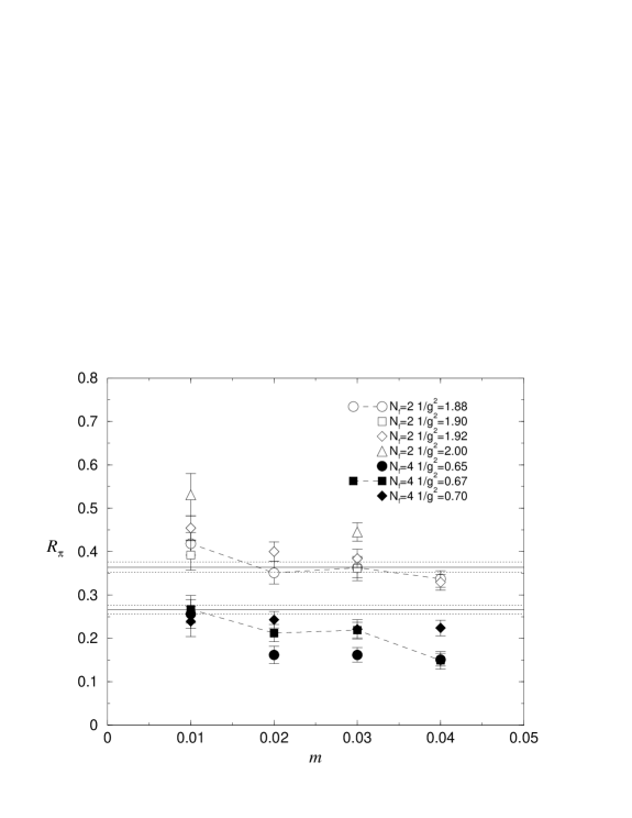
Figure 6: The ratio $R_{\pi}$ vs. $m$ for $N_{f}=2,4$ from a $16^{3}$ lattice.

The results of Fig. 5, being obtained away from the chiral limit, can serve at best as a qualitative indicator of the differences between the two models. A more quantitative guide comes from considering the ratio $R_{\pi}\equiv\chi_{l}/\chi_{t}$ as a function of bare mass $m$ [22][9]. In general $R_{\pi}$ varies with $m$, but exactly at the critical coupling, the equation of state (3.7) predicts that $R_{\pi}=\delta^{-1}$ independent of $m$. In Table 6 we present results for susceptibilities and $R_{\pi}$ for $m=0.01,\ldots,0.04$ for a range of couplings in the critical region (including some new results for $N_{f}=2$ at $1/g^{2}=1.88$); they are plotted together with results from Table 9 of ref. [9] in Fig. 6. Note that over the mass range explored $\chi$ varies by a factor of $O(3)$. Also shown in the figure are the values of $\delta^{-1}$ obtained from the equation of state fits for $N_{f}=2,4$. Within the large errors, we see that the results for $N_{f}=2$ with $1/g^{2}=1.88$ (corresponding to $t^{\prime}\simeq 0$) are roughly independent of $m$ and fall within the error band of $\delta$; for $N_{f}=4$ both independence of $m$ and agreement with $\delta$ is less convincing for the $1/g^{2}=0.67$ data (ie. $t^{\prime}\simeq-0.015$), though still plausible (it is also possible that the equation of state fits have under-estimated $\delta$ in this case). Whilst considerably more accuracy would be required before this technique became a competitive means of estimating $1/g_{c}^{2}$, in the critical region the values of $R_{\pi}$ for $N_{f}=2,4$ are clearly distinct, supporting our claim that the models’ continuum limits belong to different universality classes. One feature of Fig. 6 that remains to be explained is the systematically larger values af $R_{\pi}$ for $m=0.01$: this could be either a finite volume effect, or an artifact due to insufficient sampling of the small eigenvalue configurations noted in Fig. 4. Note that if such configurations are undersampled, the ratio $R_{\pi}$ will be over-estimated.

3.4 Spectrum

The mass spectrum of the theory is studied by fitting the time-dependence of the two-point functions with a single exponential decay. The fermion propagator has been fitted to:

$$C_{f}(t)=A\left(e^{-\mu_{R}t}-(-1)^{t}e^{-\mu_{R}(L-t)}\right),$$ (3.18)

where $\mu_{R}$ is the physical fermion mass and the minus sign between the forward and backward terms is due to our choice of antiperiodic boundary conditions in the timelike direction. Both the scalar and pion channels were fitted by the form

$$C_{l}(t)=A\left(e^{-Mt}+e^{-M(L-t)}\right).$$ (3.19)

Although the lattice data has a larger statistical noise, the masses in the three channels studied here show similar behaviours to those obtained for $N_{f}=2$ in previous publications [9].

The results are summarised in Tabs. 7, 8 and 9. The number of configurations available for each value of $1/g^{2}$ and $m$ is reported in square brackets.

Table 7: Results for the fermion spectrum.

$1/g^{2}$	$m=0.01$	$m=0.02$	$m=0.03$	$m=0.04$
$0.5$	0.65(9) [319]	0.97(20) [107]
$0.6$	0.46(5) [338]	0.43(10) [105]
$0.65$	0.42(4) [210]	0.50(5) [200]	0.48(3) [234]	0.57(3) [208]
$0.67$	0.25(7) [206]		0.45(4) [228]	0.61(5) [219]
$0.7$	0.32(3) [229]	0.37(3) [240]	0.36(2) [250]	0.43(2) [208]
$0.75$	0.16(3) [231]
$0.8$	0.16(2) [205]	0.23(2) [102]
$0.9$	0.06(1) [209]	0.14(1) [99]

Table 8: Results for the pion spectrum.

$1/g^{2}$	$m=0.01$	$m=0.02$	$m=0.03$	$m=0.04$
$0.5$	0.164(5) [313]	0.237(6) [107]
$0.6$	0.170(5) [333]	0.234(8) [105]
$0.65$	0.191(4) [209]	0.258(5) [200]	0.308(6) [234]	0.350(3) [208]
$0.67$	0.194(4) [206]	0.264(4) [200]	0.310(10) [228]	0.353(4) [219]
$0.7$	0.198(3) [221]	0.261(5) [230]	0.320(30) [250]
$0.75$	0.191(3) [228]
$0.8$	0.205(2) [201]	0.272(7) [102]
$0.9$	0.223(1) [203]	0.263(7) [99]

Table 9: Results for the scalar spectrum.

$1/g^{2}$	$m=0.01$	$m=0.02$	$m=0.03$	$m=0.04$
$0.5$	0.29(11) [305]	0.34(11) [107]
$0.6$	0.24(3) [306]
$0.65$	0.28(7) [209]	0.55(13) [200]	0.77(8) [225]	0.86(5) [208]
$0.67$	0.29(8) [202]	0.54(11) [200]	0.77(8) [192]	0.92(7) [219]
$0.7$	0.36(15) [213]	0.48(10) [215]		0.80(10)[208]
$0.75$
$0.8$	0.25(1) [201]	0.43(6) [102]
$0.9$	0.24(1) [203]	0.32(3) [99]

Table 10: Results for the vector spectrum for $m=0.01$.

$1/g^{2}$	local current	conserved current
$0.9$	0.34(8) [203]	0.31(4) [203]
$0.8$	0.97(46) [201]	0.60(14) [201]
$0.75$	0.31(17) [210]	0.50(11) [204]
$\leq 0.7$	no fit found	no fit found

Although the signal for the fermion propagator is more noisy than in the $N_{f}=2$ case, it is still possible to identify a clear increase in the fermion mass when going from the symmetric to the broken phase of the theory. The scalar propagator exhibits a very poor signal and it is often difficult to get a stable result from the fit; even with this admittedly crude accuracy it is possible to see the transition between the chirally symmetric phase where the pion and scalar are approximately degenerate, to the broken phase where the scalar is much heavier.

Figure 7: $M_{\pi}^{2}$ vs. $m$, for two different values of $\beta$ in the broken phase.

Figure 8: $M_{\pi}^{2}\langle\bar{\chi}\chi\rangle$ vs. $m$, for $\beta=0.65$.

The pion spectrum provides the most interesting information. In the broken phase and for vanishing bare mass, the pion is expected to be a massless Goldstone boson. For non-vanishing bare mass in the broken phase, the pion mass is related to the chiral condensate by a chiral Ward identity, plus the assumption of one-pole dominance:

$$M^{2}_{\pi}=\frac{Z_{\pi}}{\langle\bar{\chi}\chi\rangle}m.$$ (3.20)

Fig. 7 displays the behaviour of the pion mass squared vs. $m$. There is a satisfactory agreement with the linear behaviour expected from Eq. (3.20). A linear fit to the form:

$$M^{2}_{\pi}=\alpha m+M_{0}$$ (3.21)

yields for the pion mass in the chiral limit $M_{0}=0.008\pm 0.005$, which is within two standard deviations from the expected vanishing value. Actually, Eq. (3.20) predicts that the product of the pion mass squared times the chiral condensate is a linear function of the bare mass. The product is shown in Fig. 8. A linear fit gives a slightly negative intercept for the value of the product as $m=0$.

Finally in this subsection we discuss the spectroscopy in spin-1 channels. As described in [9], we performed measurements using both local and conserved (ie. one-link) operators. In each case the signal observed has a strong oscillatory component, being close to or consistent with zero on even timeslices, suggesting there are light states in both direct and alternating channels. This motivates the following fitting form:

$$C_{v}(t)=A(e^{-M_{d}t}+e^{-M_{d}(L-t)})+B(-1)^{t}(e^{-M_{a}t}+e^{-M_{a}(L-t)}),$$ (3.22)

which in general has four parameters. We found, however, that where fits were possible, in the symmetric phase, the two parameter fit obtained by setting $A=B$ and $M_{d}=M_{a}$ was equally plausible. For values of $1/g^{2}\leq 0.8$ the signal to noise ratio rapidly decreased and no sensible fits could be obtained for $1/g^{2}\leq 0.7$. The results are given in Table 10.

A couple of remarks about the spin-1 sector in 2+1 dimensions are worth making. First, the spin/flavor assignments are different for the two types of bilinear, the local operator projecting onto $(\gamma_{\mu}\gamma_{0}\otimes\tau_{3}^{*}\tau_{\mu})$ in direct and $(\gamma_{5}\gamma_{\mu}\gamma_{0}\otimes\tau_{3}^{*}\tau_{\mu})$ in alternating channels respectively, and the conserved onto $(\gamma_{\mu}\otimes 1\kern-4.5pt1)$ in direct and $(\gamma_{5}\gamma_{\mu}\otimes\tau_{3}^{*})$ in alternating channels, where $\mu$ labels one of the transverse directions, the first component of the tensor product acts on the four spin indices of the continuum spinor, and the second on a two-component flavor structure [17]. It can be seen that in each case the direct and alternating channels correspond to states of opposite parity, where in 2+1 dimensions in the $q$-basis the parity transformation $P$ is defined:

$$x=(x_{0},x_{1},x_{2}) \mapsto x^{\prime}=(x_{0},-x_{1},x_{2})$$

$$q(x)\mapsto(\gamma_{1}\gamma_{5}\otimes 1\kern-4.5pt1)q(x^{\prime}) \bar{q}(x)\mapsto\bar{q}(x^{\prime})(\gamma_{5}\gamma_{1}\otimes 1\kern-4.5pt1).$$ ; (3.23)

This brings us to the second point: in 2+1 dimensions the angular momentum operator $J$, which has integer eigenvalues $j$, anticommutes with $P$. Therefore the two parity eigenstates $|j,\pm\rangle=|j\rangle\pm P|j\rangle$ correspond to distinct non-null eigenstates of the Hamiltonian, since $|j\rangle$ and $P|j\rangle$ have distinct $J$ eigenvalues $j$ and $-j$. Since $P$ commutes with $H$, it follows that if parity is not spontaneously broken, the model must contain degenerate states in the massive $j\not=0$ sector of the spectrum. Such a parity doubling is observed in the glueball spectrum of SU($N$) lattice gauge theory in 2+1 dimensions [23]. In the current context we attribute the degeneracy of $M_{d}$ and $M_{a}$, as revealed by the quality of the fits of Table 10, to parity doubling. It is not clear how parity doubling is revealed in the $1/N_{f}$ expansion, which at leading order predicts a massive bound state in the $\gamma_{\mu}$ channel but not in the $\gamma_{5}\gamma_{\mu}$ channel [9].

4 $N_{f}=6$

Figure 9: Plot of $\chi_{t}$ and $\chi_{nls}$ versus $1/g^{2}$ for $N_{f}=6$ on a $16^{3}$ lattice with $m=0.01$.

Figure 10: Time history for chiral condensate measurements for $N_{f}=6$ on a $16^{3}$ lattice with $m=0.01$ and $1/g^{2}=0.38$.

Figure 11: Histogram of 478 chiral condensate measurements for $N_{f}=6$ on a $16^{3}$ lattice with $m=0.01$, $1/g^{2}=0.38$, together with a fit to a double gaussian ($\chi^{2}/\mbox{dof}=32/26$).

Figure 12: Chiral condensate versus $1/g^{2}$ for $N_{f}=6$ on a $16^{3}$ lattice, showing evidence for coexisting phases for $m=0.01$ based on double gaussian fits.

In this section we turn our attention to the case $N_{f}=6$. Although we have spent a comparable effort in accumulating data for this case, the runs are more compute intensive, firstly for the obvious reason that an extra lattice flavor implies an extra matrix inversion, and secondly because the physically interesting regime occurs at still stronger coupling – we explored the region $1/g^{2}\in[0.3,0.5]$, again with lattice size $16^{3}$ and $m=0.01$. Therefore the discussion will be more qualitative. Our primary observation is that there is still evidence for chiral symmetry breaking at strong coupling, but that the phase transition is of a different character. The evidence for a phase transition is shown in Fig. 9, where a comparison between tranverse and longitudinal non-singlet susceptibilities shows a clear separation between a chirally symmetric region ($\chi_{t}\simeq\chi_{lns}$) for $1/g^{2}>0.4$ and a chirally broken region ($\chi_{t}\gg\chi_{nls}$) for $1/g^{2}<0.35$. Consider, however, the time history of condensate measurements obtained at $1/g^{2}=0.38$ from nearly 1000 trajectories of mean length 0.9, shown in Fig. 10. It is plausible that the figure shows evidence for metastability, the system tunnelling between equilibrium states with $\langle\bar{\chi}\chi\rangle\simeq 0.05$ and $\langle\bar{\chi}\chi\rangle\simeq 0.1$. A comparison with a similar plot for the susceptibility ratio $\chi_{t}/\chi_{lns}$ reveals a correlation: when the condensate is small the ratio is close to one, suggesting that chiral symmetry is realised, whereas when the condensate is larger the ratio is much smaller, with occasional excursions to negative values, similar to the broken phase behaviour of Fig. 4. This encourages us to interpret the time history as a sequence of tunnellings between chirally symmetric and broken vacua. A histogram of the condensate measurements is shown in Fig. 11, together with a double gaussian fit of the form

$$y=A_{1}\exp\left(-{(x-\bar{x}_{1})^{2}\over{2\sigma_{1}^{2}}}\right)+A_{2}\exp\left(-{(x-\bar{x}_{2})^{2}\over{2\sigma_{2}^{2}}}\right).$$ (4.1)

The data are consistent with the twin peak structure characteristic of coexisting phases.

In Fig. 12 we plot $\langle\bar{\chi}\chi\rangle$ versus $1/g^{2}$, for $m=0.01$ and $m=0.02$ (this data taken from [9]). The $m=0.01$ data is plotted in two ways, firstly as a raw average over the whole dataset, and secondly by assuming coexistent states, with central values and standard errors taken from fits to (4.1). We found that the two procedures yield consistent results for $1/g^{2}\leq 0.35$ and $1/g^{2}\geq 0.45$; however for intermediate couplings there is a marked twin peak structure and evidence for coexisting states.

Figure 13: Time history for chiral condensate measurements for $N_{f}=6$ on a $16^{3}$ lattice with $m=0.005$ and $1/g^{2}=0.37$.

In ref. [9] we presented data for $m=0.05,\dots,0.02$ but observed no evidence for a critical point described by a Fisher plot, consistent with a second order phase transition. The new data from a larger lattice closer to the chiral limit suggest that there is indeed a phase transition, but that it is first order, as signalled by the evidence for coexisting phases in the transition region. To confirm this, of course, data from a variety of lattice volumes and bare fermion masses would be needed, requiring resources beyond the scope of the current study. We did attempt to study the transition closer to the chiral limit with some runs at $m=0.005$; a typical time history is shown in Fig. 13. The results were ambiguous, with no clear evidence for a chirally broken phase at any coupling studied down to $1/g^{2}=0.36$; this is a sure sign that any conclusions made are as yet preliminary.

5 Discussion

The main results we have found are that the $N_{f}=4$ Thirring model in three dimensions, like its $N_{f}=2$ counterpart, appears to have a continuous chiral symmetry breaking transition at strong coupling, whereas for the $N_{f}=6$ case the data suggests that the transition is first order. Moreover, the $N_{f}=4$ model has critical exponents distinct from those of $N_{f}=2$, and we expect this conclusion to be robust even if the actual numerical values of the exponents drift somewhat under more refined analyses in the future. The conclusion we draw is that both $N_{f}=2$ and $N_{f}=4$ models have interacting continuum limits, which are qualitatively, but not quantitatively similar. This is consistent with the critical flavor number $N_{fc}$, predicted in the strong coupling limit of the Schwinger-Dyson approach to the model to be approximately 4.32 in ref. [6], to be at least greater than 4. For $N_{f}=6$, on the other hand, there can be no continuum limit. It is interesting to compare our results with those found in simulations of $\mbox{QED}_{4}$; power-law fits to the equation of state [22][24] yield critical exponents which are not distinct for $N_{f}=2,4$, but studies at larger $N_{f}$ do suggest that the chiral transition eventually becomes first order in this limit [25].

It is difficult at first sight to reconcile the $N_{f}=6$ result with the Schwinger-Dyson picture, which for $N_{f}>N_{fc}$ would simply predict the absence of a stable chiral symmetry breaking solution for any finite coupling. However, as explained in [9], the lattice regularisation of the Thirring model itself contains systematic uncertainties, essentially because the interaction current in the contact term is not actually conserved. In the context of the $1/N_{f}$ expansion, this results in an uncancelled linear divergence in the calculation of the vacuum polarisation tensor, which controls the propagation of the $f\bar{f}$ state in the vector channel, and which must be absorbed by an additive renormalisation of the lattice inverse coupling constant:

$${1\over g_{R}^{2}}={1\over g^{2}}-J(m),$$ (5.1)

where $J(m)$ is calculable to leading order in $1/N_{f}$. Therefore we might expect the strong coupling limit to be attained for $1/g^{2}=J(m)$; indeed for $1/g^{2}<J(m)$ the $1/N_{f}$ expansion of the lattice model is not unitary. What the results in this paper show is that the true picture at small $1/g^{2}$ is not described by the $1/N_{f}$ expansion, probably because it assumes the wrong vacuum state, ie. one where chiral symmetry is realised. Instead, at strong couplings, or equivalently for sufficiently many fermion flavors, the chiral transition becomes first order, invalidating approaches such as either the $1/N_{f}$ expansion or the Schwinger-Dyson equation, which both rely on the applicability of continuum field theory. We can, however, retain the notion of a critical flavor number $N_{fc}$, such that chiral symmetry breaking solutions such as those of [6] are applicable, and RG fixed points exist for $N_{f}<N_{fc}$. In this case our main result can be stated:

$$4<N_{fc}<6.$$ (5.2)

Work is in progress, using a generalisation of the numerical algorithm to allow for non-integer $N_{f}$, to explore further the phase diagram of the model in the $(1/g^{2},N_{f})$ plane, and hopefully to pin down the value of $N_{fc}$ more precisely [26].

Finally, what of the theory with $N_{f}\simeq N_{fc}$? According to [6], at this point we expect the induced physical scale (inverse correlation length) $\mu$ to scale in an essentially singular way:

$${\mu\over\Lambda}\propto\exp\left(-{{2\pi}\over\sqrt{{N_{fc}\over N_{f}}-1}}\right),$$ (5.3)

a form of scaling characteristic of a conformal phase transition [10]. Indeed, following the discussion of the introduction, it is precisely for $N_{f}=N_{fc}$ that we might expect the Thirring model and $\mbox{QED}_{3}$ to coincide [11][9]. On the assumption that this limit might be approached along a smooth trajectory corresponding to a line of phase transitions in the $(1/g^{2},N_{f})$ plane, and that critical exponents vary continuously along this line, then we have an apparent contradiction; our numerical results suggest that the exponent $\delta$ increases as $N_{f}\nearrow N_{fc}$, whereas for a chiral transition described by essential singularity, such as an asymptotically-free theory, or the quenched gauged NJL model [19], $\delta$ is expected to take the value 1, and hence decrease as this limit is approached. Therefore we conclude that our simulation results do not appear to support the existence of a conformal phase transition.

6 Acknowledgements

SJH was supported in part by a PPARC Advanced Fellowship, and in part by the TMR-network “Finite temperature phase transitions in particle physics” EU-contract ERBFMRX-CT97-0122. LDD is supported by PPARC under grants GR/L56329 and GR/L29927. Some of the computing work was performed using the resources of the UKQCD collaboration under PPARC grants GR/K41663, GR/K455745 and GR/L29927. We have enjoyed discussing aspects of this work with Biagio Lucini, Jiří Jersák and Wolfgang Franzki.

References

-
[1]
T. Banks and A. Zaks, Nucl. Phys. B196 (1982) 189;
T.W. Appelquist, J. Terning and L.C.R. Wijewardhana, Phys. Rev. Lett. 77 (1996) 1214. - [2] N. Seiberg, Nucl. Phys. B435 (1995) 129.
-
[3]
M. Alford, K. Rajagopal and F. Wilczek, Phys. Lett. B422
(1998) 247; Nucl. Phys. B537 (1999) 443;
T. Schäfer and F. Wilczek, hep-ph/9811473. -
[4]
T.W. Appelquist, M.J. Bowick, D. Karabali and L.C.R.
Wijewardhana, Phys. Rev. D33 (1986) 3704, 3774;
M.R. Pennington and D. Walsh, Phys. Lett. B253 (1991) 246;
P. Maris, Phys. Rev. D54 (1996) 4049. - [5] M. Gomes, R.S. Mendes R.F. Ribeiro and A.J. da Silva, Phys. Rev. D43 (1991) 3516.
- [6] T. Itoh, Y. Kim, M. Sugiura and K. Yamawaki, Prog. Theor. Phys. 93 (1995) 417.
- [7] D.K. Hong and S.H. Park, Phys. Rev. D 49 (1994) 5507.
- [8] K.-I. Kondo, Nucl. Phys. B 450 (1995) 251.
-
[9]
L. Del Debbio, S.J. Hands, Phys. Lett. B373
(1996) 171;
L. Del Debbio, S.J. Hands and J.C. Mehegan, Nucl. Phys. B502 (1997) 269;
L. Del Debbio, talk presented at Lattice ’97, Symposium on Lattice Field Theory, Edinburgh, Scotland, hep-lat/9709034. - [10] V.A. Miranskii and K. Yamawaki, Phys. Rev. D55 (1997) 5051.
- [11] V.P. Gusynin, V.A. Miranskii and A.V. Shpagin, Phys. Rev. D58 (1998) 085023.
-
[12]
G. Parisi, Nucl. Phys. B 100 (1975) 368;
S. Hikami and T. Muta, Prog. Theor. Phys. 57 (1977) 785;
Z. Yang, Texas preprint UTTG-40-90 (1990);
S.J. Hands, Phys. Rev. D51 (1995) 5816. - [13] I.J.R. Aitchison and N.E. Mavromatos, Phys. Rev. B53 (1996) 9321.
- [14] I.M. Barbour, N. Psycharis, E. Focht, W. Franzki and J. Jersák, Phys. Rev. D58 (1998) 074507.
- [15] C. Frick and J. Jersák, Phys. Rev. D52 (1995) 340.
- [16] A. Kocić, Phys. Lett. B281 (1992) 309.
- [17] C.J. Burden and A.N. Burkitt, Europhys. Lett. 3 (1987) 545.
- [18] E. Focht, J. Jersák and J. Paul, Phys. Rev. D53 (1996) 4616.
- [19] E. Dagotto, S.J. Hands, A. Kocić and J.B. Kogut, Nucl. Phys. B347 (1990) 217.
- [20] see e.g. J. Zinn-Justin, Quantum Field Theory and Critical Phenomena (Oxford Science Publications, Oxford, 1989), chap. 25, and references therein.
- [21] J. Cox, W. Franzki, J. Jersák, C.B. Lang and T. Neuhaus, Nucl. Phys. B532 (1998) 315.
-
[22]
A. Kocić, J.B. Kogut and K.C. Wang, Nucl. Phys. B398 (1993)
405;
M. Göckeler, R. Horsley, V. Linke, P.E.L. Rakow, G. Schierholz and H. Stüben, Nucl. Phys. B487 (1997) 313. - [23] M.J. Teper, Phys. Rev. D59 (1999) 014512.
- [24] S.J. Hands, A. Kocić, J.B. Kogut, R.L. Renken, D.K. Sinclair and K.C. Wang, Nucl. Phys. B413 (1994) 503.
- [25] J.B. Kogut and K.C. Wang, Phys. Rev. D53 (1996) 1513.
- [26] S.J. Hands and B. Lucini, in preparation.