Various Representations of Infrared Effective Lattice $\mathbf{SU(2)}$ Gluodynamics

Abstract

We study various representations of infrared effective theory of $SU(2)$ gluodynamics starting from the Abelian monopole action derived recently by numerical calculations in the Maximal Abelian projection. In particular we derive the string model and the dual Abelian-Higgs (dual Ginzburg-Landau) model which corresponds to infrared $SU(2)$ gluodynamics. It occurs that the classical string tension in the string model is of the same order as the string tension in quantum $SU(2)$ gluodynamics.
$PACS$: 12.38.Gc, 11.15.Ha
$Keywords$: lattice $SU(2)$ QCD; abelian projection; abelian monopole; dual transformation; dual Ginzburg-Landau model; string model

I Introduction

The knowledge of an infrared effective theory of QCD would be very important for the analytical description of hadron physics. Before the derivation of a low-energy effective theory of QCD we have to explain the most important non-perturbative phenomenon, the quark confinement. Wilson’s lattice formulation [1] shows that the confinement is a property of a non-Abelian gauge theory of strong interactions. At strong coupling the confinement is proven analytically. At weak coupling (corresponding to the continuum limit) there are a lot of numerical calculations showing the confinement of color. The mechanism of confinement is still not well understood. One of approaches to the confinement problem is based on the searching of the relevant dynamical variables and construction of an effective theory for these variables.

From this point of view the idea proposed by ’t Hooft [2] is very promising. The proposal is based on the fact that after a partial gauge fixing (Abelian projection) the $SU(N)$ gauge theory is reduced to an Abelian $U(1)^{N-1}$ theory with $N-1$ different types of abelian monopoles. Then the confinement of quarks can be explained as the dual Meissner effect which is due to the condensation of these monopoles. The QCD vacuum is dual to the ordinary superconductor: the monopoles playing the role of the Cooper pairs. The confinement occurs due to the formation of a string with the electric flux between quark and anti-quark, this string is a dual analogue of the Abrikosov string [3]. The described mechanism of confinement is usually called the dual superconductor mechanism.

There are many ways to perform the Abelian projection, but only in the Maximal Abelian (MA) gauge [4] many numerical results support the dual superconductor picture of confinement [5] (see, for example, reviews [6, 7]). These results suggest that the Abelian monopoles which appear after the Abelian projection of QCD, are relevant dynamical degrees of freedom in the infrared region.

In compact QED, due to the periodicity of the gauge field, there exist monopole excitations which are responsible for “charge confinement”[8]. The effective theory in terms of monopoles was studied both analytically [9] and numerically [10]. It was found [10] that the monopole action contains all information about confinement in this theory. The role of monopoles in the confinement in non-Abelian gauge theories is also non-trivial. The well known example is confinement in the 3-dimensional Georgi-Glashow model [11] which is due to the ’t Hooft-Polyakov monopole [12].

The effective monopole action for the MA projection of $SU(2)$ gluodynamics was obtained by Shiba and Suzuki [10] using the generalized Swendsen method [13]. Assuming that the action contains only terms which are quadratic in monopole currents, they found that the action has the form theoretically predicted by Smit and van der Sijs [14]. However the considered physical distances are rather small and the main assumption, the quadratic form of the monopole interactions, is not well justified.

The monopole action which contains only quadratic terms corresponds to the dual Abelian Higgs theory in the London limit, the lagrangian of which is

$$L_{dual}(A,\Phi)=\frac{1}{4\,g^{2}_{\mathrm{m}}}{(\partial_{[\mu,}A_{\nu]})}^{2}+\frac{1}{2}{|(\partial_{\mu}+iA_{\mu})\Phi|}^{2}+\lambda{({|\Phi|}^{2}-\eta^{2})}^{2}\,,$$ (1)

where $A_{\mu}$ is the dual gauge field and $\Phi$ is the monopole field. In the London limit, $\lambda\to+\infty$, the radial part of the monopole field is frozen, $|\Phi|=\eta$. As we discuss in Section II the corresponding monopole action in the lattice regularization is [14, 15]:

$$S_{\mathrm{mon}}(^{*}\!k)=\frac{g_{\mathrm{m}}^{2}}{2}\left(\,{}^{*}\!k,\Delta^{-1}{\,{}^{*}\!k}\right)+p\|{\,{}^{*}\!k}\|^{2}\,,$$ (2)

where the first term in the r.h.s. corresponds to the Coulomb–interaction of monopole currents ${}^{*}k$, $\Delta^{-1}$ is the inverse lattice Laplacian. The last term in (2) is proportional to the length of the monopole trajectory. In (2) and below we use the notations of the formalism of the differential forms on the lattice [16], for the brief explanation of the notations see Appendix A of the review [7].

It is not necessary that $SU(2)$ gluodynamics in the abelian projection corresponds to the dual Abelian Higgs theory (1) in the London limit ($\lambda\to+\infty$). The finite value of $\lambda$ was firstly discussed in ref. [17] where the dual Ginzburg-Landau (DGL) theory was studied as an effective theory of QCD. From the analysis of the experimental data it was found that DGL is near the border of type II and type I superconductor (Bogomol’ny limit). The similar conclusion has been made in Ref. [18] where a non-abelian dual theory of QCD has been considered. At present there are a lot of numerical data [19] showing that the lattice gluodynamics is in a sense equivalent at large distances to the dual Abelian Higgs model near the Bogomol’ny limit. In the present publication we present new facts in favor of this statement.

Below we show that for finite coupling $\lambda$ the additional terms in the monopole action (2) appear. This is consistent with the recent numerical analysis of the monopole interactions on the large ($48^{4}$) lattice performed in ref. [20]; where it was shown that the effective monopole action contains not only quadratic interaction but also 4- and 6-point couplings of the monopole currents. The action seems to satisfy the scaling behavior, that is, it depends on the physical length $b=na(\beta)$ alone, where $n$ is the number of the blocking transformations and $a(\beta)$ is the lattice spacing. This scaling behavior is consistent with the behavior of the perfect action on the renormalized trajectory. In Section III, we analyze the new numerical results on the monopole action. The couplings of the monopole action are determined by Swendsen’s method from the monopole current configurations extracted in the MA projection from $SU(2)$ lattice gauge fields.

In Section IV we derive the string action from the monopole action. We thus obtain the effective string action for lattice gluodynamics. There exist many attempts to relate the string theory with a local field theory. Nielsen and Olesen[21] have found quantized magnetic flux lines as static solutions in the Abelian Higgs model, they also mentioned that strings behave similarly to the Nambu string [22]. Förster et al. [23] have proved that, in the zero-width limit, flux lines move like Nambu strings. Using the collective coordinate formalism [23, 24, 25] they have constructed an effective string model. There are many speculations about the possible relation between string theory and non-Abelian field theory [26].

In the London limit ($\lambda\to\infty$) the Abelian Higgs model, can be exactly rewritten as the string theory with a non-local action [25, 27, 28, 29]. Thus in the London limit the infrared effective theory of QCD developed in Ref. [17] can be explicitly rewritten as a string theory in the London limit. This fact is natural since the dual picture of QCD vacuum suggests the formation of QCD strings. The formation of string between quark and anti-quark leads to the confinement phenomenon. The effective action for the QCD string contains in addition to the Nambu-Goto term the so-called rigidity term [27, 30, 31] and other more complicated interactions.

The main task of this publication is to interrelate various models (monopole current model, string model, Abelian Higgs model and others) which are equivalent to lattice gluodynamics. In Section II we briefly discuss various models which are equivalent to the quadratic monopole action (2). In Section III we calculate the couplings for the monopole action which corresponds to $SU(2)$ gluodynamics in the MA projection. In Section IV we discuss the effective string action corresponding to lattice $SU(2)$ gluodynamics. In Section V we discuss the DGL theory (an effective dual Abelian-Higgs model) which is equivalent to the theory with the monopole action described in Section III. We study this effective model in three different regions of coupling parameters of the DGL theory. The details of the calculations are collected in Appendices A–B. The conclusions are given in Section VI.

II MONOPOLE ACTION IN THE LONDON LIMIT

In this Section we discuss several representations for the theory with the quadratic monopole action (2). The basic method we use is a generalization of the transformation of Berezinski [32], Kosterlitz and Thouless [33] and the duality transformation originally suggested by Kramers and Wannier [34] for the 2–dimensional Ising model. The Berezinski–Kosterlitz–Thouless (BKT) transformation relates the two-dimensional $XY$ model and the “vortex + spinwave” system [32, 33, 35]. Banks et. al extended this method to the system with Abelian gauge symmetry, and found a “monopole + photon” representation of lattice gauge theory in 3-dimensions and a “monopole current + photon” representation in 4-dimensions [9]. The monopole partition function corresponding to monopole action (2) can be transformed into the partition function of the dual Abelian Higgs model [14, 15] and into the partition function for the string theory of hadrons on the lattice [29].

The partition function in the case of quadratic monopole action is:

$${\cal Z}^{\mathrm{mon}}=\sum_{\stackrel{{\,{}^{*}\!k(\,^{*}\!c_{1})\in{Z\!\!\!Z}}}{{\delta\,^{*}\!k=0}}}\exp\left(-S_{\mathrm{mon}}(^{*}\!k)\right)\,,$$ (3)

where the monopole action $S_{\mathrm{mon}}$ is defined by eq.(2). The condition $\delta{}^{*}k=0$ means that we sum over all closed (conserved) currents on the dual lattice. Applying the inverse duality transformation (see Appendix A) to eq.(3) we get the partition function:

$${\cal Z}^{\mathrm{AH}}=\int\limits_{-\infty}^{\infty}D\,^{*}\!A(\,^{*}\!c_{1})\int\limits_{-\pi}^{\pi}D{\,{}^{*}\!\varphi}(\,^{*}\!c_{0})\sum_{\,{}^{*}\!l(\,^{*}\!c_{1})\in{Z\!\!\!Z}}\!\!\!\!\!\!\!\quad\exp\left\{-\frac{1}{2g_{\mathrm{m}}^{2}}\|d\,^{*}\!A\|^{2}-\frac{1}{4p}{\|}d\,^{*}\!\varphi+2\pi\,^{*}\!l-\,^{*}\!A\|^{2}\right\}\,.$$ (4)

Now we show that (4) is the lattice version of the (dual) Abelian Higgs model in the London limit. The direct lattice analogue of the action of the Abelian Higgs model (1) is [36]:

$${\cal S}^{\rm A.H.}[A,\Phi] = \frac{1}{2g^{2}_{\mathrm{m}}}{||{\rm d}A||}^{2}-\gamma\sum_{x,\mu}\left({\Phi}^{*}(x)U_{\mu}(x)\Phi(x+\hat{\mu})+h.c.\right)$$ (6)

$$+\lambda\sum_{x}\left({\Phi}^{*}(x)\Phi(x)-1\right)^{2}+\sum_{x}{\Phi}^{*}(x)\Phi(x),$$

where $U=\exp\left(iA_{\mu}\right)$ is the dual gauge field, ${\rm d}A\equiv A_{\rm P}$ is the field strength tensor and $\Phi(x)=\rho_{x}\exp\left(i\varphi_{x}\right)$ is the complex Higgs field.

Action (6) can be rewritten as follows

$${\cal S}^{\rm A.H.}[A,\rho,\varphi] = \frac{1}{2g^{2}_{\mathrm{m}}}\left\|{\rm d}A\right\|^{2}-2\gamma\sum_{x,\mu}\rho_{x}\rho_{x+\hat{\mu}}\cos\left\{\left(d\varphi\right)_{x,\mu}+A_{\mu}\right\}$$ (8)

$$+\lambda\sum_{x}\left(\rho_{x}^{2}-1\right)^{2}+\sum_{x}\rho_{x}^{2}.$$

It is convenient to modify the action using the Villain formulation by replacing $\exp\left\{\alpha\cos\psi\right\}\to\sum_{l\in{Z\!\!\!Z}}\exp\left\{\alpha-\frac{\alpha}{2}\left(\psi+2\pi l\right)^{2}\right\}$, and the partition function of the Abelian Higgs model becomes:

$${\cal Z}^{\rm A.H.}=\int\limits_{-\infty}^{+\infty}{\cal D}A\int\limits_{-\pi}^{+\pi}{\cal D}\varphi\int\limits_{0}^{+\infty}{\cal D}\rho^{2}\sum_{l\in{Z\!\!\!Z}}\exp\left\{-\frac{1}{2g^{2}_{\mathrm{m}}}\left\|{\rm d}A\right\|^{2}\right.-\gamma\sum_{x,\mu}\rho_{x}\rho_{x+\hat{\mu}}\left(A_{\mu}+\left(d\varphi\right)_{\mu}+2\pi l\right)^{2}$$ (9)

$$- \left.\gamma\sum_{x,\mu}\left(\rho_{x}-\rho_{x+\hat{\mu}}\right)^{2}-\sum_{x}(\left(1-8\gamma\right)\rho_{x}^{2}+\lambda\left(\rho_{x}^{2}-1\right)^{2})\right\}.$$ (10)

The continuum limit of the Villain action is still the action defined by eq.(1). In the London limit $\lambda\to\infty$, $\rho_{x}=1$ and the partition function (10) is equivalent to the partition function (4). The relation of the lattice lagrangian which enters the partition function (4) and the continuum lagrangian (1) of the abelian Higgs model is obvious. $d^{*}\!A$ is an analog of the dual field strength tensor $\partial_{[\mu,}A_{\nu]}$ and the term ${\|}d\,^{*}\!\varphi+2\pi\,^{*}\!l-\,^{*}\!A\|^{2}$ corresponds to ${|(\partial_{\mu}+iA_{\mu})\Phi|}^{2}$. The summation over $l$ appears due to the compactness of the phase $\varphi$ of the Higgs field $\Phi=|\Phi|\,e^{i\varphi}$. The radial component $|\Phi|$ of the Higgs field is frozen, since $\lambda\to+\infty$.

Performing the BKT transformation for the field $\,{}^{*}\!\varphi(\,^{*}\!c_{0})$ in eq.(4) we get the string representation of the model (see Appendix A for details) [29]:

$${\cal Z}^{\mathrm{str}}=\sum_{\sigma(c_{2})\in{Z\!\!\!Z},\delta\sigma=0}\exp\left\{-\frac{\pi^{2}}{p}\left(\sigma,\left(\Delta+M^{2}_{A}\right)^{-1}\sigma\right)\right\}\,,$$ (11)

where

$$M^{2}_{A}=\frac{g_{\mathrm{m}}^{2}}{2p}\,,$$ (12)

is the mass of the dual gauge field $A$. The integer-valued 2-form $\sigma$ represents the closed world surface of the string formed by the electric flux. The propagator $\left(\Delta+M^{2}_{A}\right)^{-1}$ in eq.(11) means that the string elements interact via the exchange of the massive gauge boson. The condition $\delta\sigma=0$ means that the world sheets of Nielsen-Olesen strings must form closed surfaces. This interpretation of $\sigma$ is clear from the following considerations. Consider in representation (4) the expectation value of the ’t Hooft loop operator which introduces the quark–anti-quark pair:

$$<H({\cal C})> = \frac{1}{{\cal Z}^{\mathrm{A.H.}}}\int\limits_{-\infty}^{\infty}D\,^{*}\!A(\,^{*}\!c_{1})\int\limits_{-\pi}^{\pi}D{\,{}^{*}\!\varphi}(\,^{*}\!c_{0})\sum_{\,{}^{*}\!l(\,^{*}\!c_{1})\in{Z\!\!\!Z}}$$ (14)

$$\exp\left\{-\frac{1}{2g_{\mathrm{m}}^{2}}\|d\,^{*}\!A+2\pi^{*}\!S_{\cal C}\|^{2}-\frac{1}{4p}{\|}d\,^{*}\!\varphi+2\pi\,^{*}\!l-\,^{*}\!A\|^{2}\right\}$$

$$= \frac{1}{{\cal Z}^{\mathrm{str}}}\sum_{\stackrel{{\scriptstyle\sigma(c_{2})\in{Z\!\!\!Z}}}{{\delta\sigma={\cal C}}}}\exp\left\{-\frac{\pi^{2}}{p}\left(\sigma,\left(\Delta+M^{2}_{A}\right)^{-1}\sigma\right)-\frac{2\pi^{2}}{g^{2}_{\mathrm{m}}}\left({\cal C},\left(\Delta+M^{2}_{A}\right)^{-1}{\cal C}\right)\right\}\,,$$ (15)

here ${\cal C}$ is the quark-antiquark trajectory; $S_{\cal C}$ is an arbitrary surface spanned on the loop ${\cal C}$: $\delta S_{\cal C}={\cal C}$. The summation in (15) is over all closed surfaces (virtual glueballs). Effectively it means that we sum also over all surfaces spaned on the contour ${\cal C}$. Thus $\sigma$ represents the worldsheet of the color electric flux.

Finally we mention that the abelian monopoles in model (3) can be considered as defects in a compact gauge theory similarly to the compact QED. The corresponding ”compact QED” representation of the partition function (3) is:

$${\cal Z}^{\mathrm{compact}}=\int\limits^{+\pi}_{-\pi}D\theta\,\sum\limits_{n(c_{2})\in{Z\!\!\!Z}}\exp\Bigl{\{}-\frac{g^{2}_{\mathrm{m}}}{8\pi^{2}}{||{\rm d}\theta+2\pi n||}^{2}-\frac{p}{4\pi^{2}}({\rm d}\theta+2\pi n,\Delta({\rm d}\theta+2\pi n))\Bigr{\}}\,,$$ (16)

where $n$ is the integer–valued two–form and the action is invariant under $U(1)$ gauge transformations, $\theta\to(\theta+{\rm d}\alpha)\,{\mathrm{mod}}2\pi$. Applying the standard BKT transformation [9, 32, 33] to the field $\theta$, $\theta+2\pi n=\theta_{n.c.}+2\pi\Delta^{-1}\delta k$, (${}^{*}k$ is the closed monopole trajectory, $\delta{}^{*}k=0$, and $\theta_{n.c.}$ is a non-compact field), we get the partition function (3) from ${\cal Z}^{\mathrm{compact}}$  (16).

III THE MONOPOLE ACTION FROM GLUODYNAMICS

In this Section we present the results of the numerical investigation of the effective monopole action in $SU(2)$ gluodynamics. We generate the $SU(2)$ gauge fields on $48^{4}$ lattice, perform the Maximal Abelian gauge fixing and extract monopole currents.

As we discuss in the Introduction, there are strong indications [17, 18, 19], that the gauge boson mass is of the order of the Higgs boson mass in the effective Abelian Higgs model which corresponds to the infrared lattice $SU(2)$ gluodynamics. Thus $\lambda$ is finite in the effective action (1) and (8). As we show in Section V for finite $\lambda$ the monopole action contains $N$-point ($N=2,4,6,\dots$) interactions. Hence we have fitted the numerical data for the monopole currents by the partition function:

$${\cal Z}^{\rm mon}=\sum_{{{}^{*}k\in{Z\!\!\!Z}}\atop{\delta{}^{*}k=0}}\exp\left\{-S^{\rm mon}\left[{}^{*}k\right]\right\}\,,$$ (17)

where the action ${\cal S}^{\rm mon}[{}^{*}k]$ contains $2$-,$4$- and $6$- point interactions of the monopole currents:

$${\cal S}^{\rm mon}[{}^{*}k]=\frac{g_{\rm m}^{2}(b)}{2}\left({}^{*}k,\Delta^{-1}{}^{*}k\right)+p(b)\left\|{}^{*}k\right\|^{2}-q(b)\sum_{x}\left(\sum_{\mu=-4}^{4}{}^{*}k_{x,\mu}^{2}\right)^{2}$$ (18)

$$+ r(b)\sum_{x}\sum_{\mu,\nu,\delta=-4}^{4}{}^{*}k_{x,\mu}^{2}{}^{*}k_{x,\nu}^{2}\left(3{}^{*}k_{x,\delta}^{2}+{}^{*}k_{x+\nu,\delta}^{2}\right)+\sum_{i}f_{i}(b)S_{2}^{(i)}[{}^{*}k]\,.$$ (19)

The monopole currents ${}^{*}k$ are defined on the dual lattice. They are integer valued and conserved ($\delta\,^{*}k=0$). $S_{2}^{(i)}[k]$ are additional $2$-point interactions [10] of monopole currents which are introduced to check whether there are any corrections to the Coulomb interaction $\left({}^{*}k,\Delta^{-1}{}^{*}k\right)$. Our numerical results show that these corrections are negligibly small in the infrared region, and we neglect them in what follows.

To determine coefficients $g_{\mathrm{m}}^{2}(b)$, $p(b)$, $q(b)$, $r(b)$ numerically we use the modified Swendsen method [10, 13] (which is a kind of inverse Monte Carlo method) for monopole currents in the MA projection of lattice $SU(2)$ gluodynamics [20]. In order to study the renormalization group evolution of the effective action in the infrared region we consider the $n$-fold extended type-II monopole currents [37] ($n=1,2,3,4,6,8$) which emerge from the block-spin transformation on the dual lattice.

It is interesting that the couplings of the monopole action (19) seem to depend only on the physical length $b=n\cdot a(\beta)$ when $n$ is larger than $3$. This fact means that we are working on the renormarized trajectory. In order to express $b$ in terms of the physical (dimensional) units we measure the dimensionless string tension $\tilde{\kappa}(\beta)$ (in lattice units)[20]. Then $a\left(\beta\right)=\sqrt{\tilde{\kappa}(\beta)/\kappa_{\mathrm{phys}}}$, where $\kappa_{\mathrm{phys}}$ is the physical string tension (which is about $440$ MeV in $SU(3)$ QCD).

The best fit for the renormalized couplings to numerical data for $g_{\mathrm{m}}^{2}(b)$, $p(b)$, $q(b)$, $r(b)$ gives:

$$\frac{g_{\rm m}^{2}(b)}{2} = 0.300(22)\left(\frac{4\pi}{g\left(b\right)}\right)^{2},$$ (20)

$$p(b) = \frac{0.527(25)}{b^{3.53(7)}},$$ (21)

$$q(b) = \frac{0.0178(15)}{b^{6.18(13)}},$$ (22)

$$r(b) = \frac{0.83(8)\times 10^{-4}}{b^{10.05(17)}},$$ (23)

where

$$g^{-2}(b)=\frac{11}{24\pi^{2}}\ln\left(1+\frac{1}{\left(b\Lambda\right)^{2}}\right)+\frac{17}{44\pi^{2}}\ln\left[1+\ln\left(1+\frac{1}{\left(b\Lambda\right)^{2}}\right)\right],$$ (24)

$$\Lambda=0.88(7).$$ (25)

These fits are shown in Figures 1-4. The $b$-dependence(24) of $g$ is consistent with the 2-loop running coupling for the small $b$ region and reproduces the experimental (numerical) power behavior for the large $b$ region.

IV THE LATTICE QCD STRING

It follows from Figure 4 that the 6-point interaction is negligibly small for $b\geq 1.0\left[\kappa^{-1/2}\right]$. We neglect it for simplicity in what follows, since we are interesting in the infrared effective theory which corresponds to large $b$ values. The introduction of the small 6-point interaction is not difficult. Our starting point is the monopole partition function and we discuss the string representation for the monopole action (cf. eq.(19)):

$${\cal Z}^{\mathrm{mon}}=\sum_{{{}^{*}k(^{*}c1)\in{Z\!\!\!Z}}\atop{\delta{}^{*}k=0}}\exp\left\{-\frac{g_{\mathrm{m}}^{2}}{2}\left({}^{*}k,{\Delta}^{-1}{}^{*}k\right)-p{||{}^{*}k||}^{2}+q\sum_{x}\left(\sum_{\mu=-4}^{4}{}^{*}k_{x,\mu}^{2}\right)^{2}\right\}.$$ (26)

The partition function (26) is divergent at large densities of the monopole currents ${}^{*}k$ due to positivity of the coefficient $q$. However, the partition function is a part of the total partition function with $n$-point, $n\geq 6$, being omitted. Due to the higher–point interactions the total partition function is convergent and the expectation value of the monopole density is finite. Therefore at sufficiently small values of $q$ we can treat the coupling $q$ in eq.(26) perturbatively:

$${\cal Z}^{\mathrm{mon}} = \sum_{{{}^{*}k(^{*}c1)\in{Z\!\!\!Z}}\atop{\delta{}^{*}k=0}}\exp\Bigl{\{}-\frac{g_{\mathrm{m}}^{2}}{2}\left({}^{*}k,{\Delta}^{-1}{}^{*}k\right)-p{||{}^{*}k||}^{2}\Bigr{\}}\cdot\prod\limits_{x}\Bigl{(}1+q\sum_{x}\left(\sum_{\mu=-4}^{4}{}^{*}k_{x,\mu}^{2}\right)^{2}+O(q^{2})\Bigr{)}$$ (27)

$$= \prod\limits_{x}\Bigl{(}1+q\left(\sum_{\mu=-4}^{4}\frac{\delta^{2}}{\delta B^{2}_{x,\mu}}\right)^{2}+O(q^{2})\Bigr{)}{\cal Z}[B]{\Bigl{|}}_{B=0}\,,$$ (28)

where the generating partition function is:

$${\cal Z}[B]=\sum_{{{}^{*}k(^{*}c1)\in{Z\!\!\!Z}}\atop{\delta{}^{*}k=0}}\exp\Bigl{\{}-\frac{g_{\mathrm{m}}^{2}}{2}\left({}^{*}k,{\Delta}^{-1}{}^{*}k\right)-p{||{}^{*}k||}^{2}+(i{}^{*}k,{}^{*}B)\Bigr{\}}\,.$$ (29)

Using the transformations of Appendix A we get:

$${\cal Z}[B]=\sum_{\sigma(c_{2})\in{Z\!\!\!Z},\delta\sigma=0}\exp\left\{-\frac{1}{4p}\left(2\pi\sigma+{\rm d}B,\left(\Delta+M^{2}_{A}\right)^{-1}(2\pi\sigma+{\rm d}B\right)\right\}\,.$$ (30)

Substituting this expression in eq.(28) we get the following partition function

$${\cal Z}^{\mathrm{mon}}\propto{\cal Z}^{\mathrm{str}}=\sum_{\sigma(c_{2})\in{Z\!\!\!Z},\delta\sigma=0}\exp\{-S^{(0)}(\sigma)-qS^{(1)}(\sigma)+O(q^{2})\}\,,$$ (31)

where

$$S^{(0)}(\sigma) = \frac{\pi^{2}}{p}(\sigma,\left(\Delta+M^{2}_{A}\right)^{-1}\sigma)\,,$$ (32)

$$S^{(1)}(\sigma) = \sum\limits_{x}\sum^{4}_{\mu,\nu=-4}\Bigl{(}2T_{x,\nu;x,\nu}E^{2}_{x,\mu}+4E_{x,\mu}T_{x,\mu;x,\nu}E_{x,\nu}-E^{2}_{x,\mu}E^{2}_{x,\nu}\Bigr{)}\,,$$ (33)

$$E_{x,\mu} = \frac{\pi}{p}{\Bigl{(}{(\Delta+M^{2}_{A})}^{-1}\delta\sigma\Bigr{)}}_{x,\mu}\,,$$ (34)

$$T_{x,\mu;y,\nu} = \frac{1}{2p}{\Bigl{(}\delta{(\Delta+M^{2}_{A})}^{-1}{\rm d}\Bigr{)}}_{x,\mu;y,\nu}\,.$$ (35)

By a straightforward calculation one can show that

$$T_{x,\mu;x,\nu} = \frac{6}{2p}({\cal D}_{M_{A}}(0,0,0,0)-{\cal D}_{M_{A}}(1,0,0,0))\quad\quad(\mbox{ for $\mu=\nu$ })$$ (36)

$$= \frac{1}{2p}(2{\cal D}_{M_{A}}(1,0,0,0)-{\cal D}_{M_{A}}(0,0,0,0)-{\cal D}_{M_{A}}(1,1,0,0))\quad\quad(\mbox{ for $\mu\neq\nu$ })\,,$$ (37)

$$= 0\quad\quad(\mbox{ for $\mu=-\nu$ })\,,$$ (38)

where $M_{A}$ is effective dual gauge boson mass (12) and ${\cal D}_{M_{A}}(x)={(\Delta+M^{2}_{A})}^{-1}(x)$ is the massive propagator. Combining eqs.(31)-(37) we get the string action:

$${\cal S}^{\mathrm{str}}[\sigma] = \frac{\pi^{2}}{p}(\sigma,{\cal D}_{M_{A}}\sigma)+\frac{60q\pi^{2}}{p^{3}}({\cal D}_{M_{A}}(0,0,0,0)$$ (42)

$$-{\cal D}_{M_{A}}(1,0,0,0))\cdot\sum\limits_{x}\sum\limits^{4}_{\mu=-4}{\Bigl{(}{\cal D}_{M_{A}}\delta\sigma\Bigr{)}}^{2}_{x,\mu}+\frac{2q\pi^{2}}{p^{3}}(2{\cal D}_{M_{A}}(1,0,0,0)$$

$$-{\cal D}_{M_{A}}(0,0,0,0)-{\cal D}_{M_{A}}(1,1,0,0))\cdot\sum\limits_{x}\sum\limits^{4}_{\mu\nu=-4\atop{(\mu\neq\nu)}}{\Bigl{(}{\cal D}_{M_{A}}\delta\sigma\Bigr{)}}_{x,\mu}{\Bigl{(}{\cal D}_{M_{A}}\delta\sigma\Bigr{)}}_{x,\nu}$$

$$-\frac{q\pi^{4}}{p^{4}}\sum\limits_{x}{\Bigl{(}\sum\limits^{4}_{\mu=-4}{\Bigl{(}{\cal D}_{M_{A}}\delta\sigma\Bigr{)}}^{2}_{x,\mu}\Bigr{)}}^{2}+O(q^{2})\,,$$

The leading part of the action (the first term in the r.h.s. of  (42)) comes from the self-interaction and from the Coulomb interaction of the monopole currents (see Section II); there are also corrections due to ${}^{*}k^{4}$-interaction. Action (42) is calculated as an expansion over the parameter $q$ which is small in the large $b$ region. It is interesting to note that the 4-point interaction in the monopole action induces the 4-interaction in the string action (last term in eq.(42)). The presence of the 4-point term is an indication of the finiteness of the dual Higgs boson. Thus the local four–point monopole interaction leads to the non–local four–point string interaction.

The classical string tension is defined as follows:

$$S(\sigma^{\mathrm{flat}})=\kappa_{\mathrm{th}}\cdot Area(\sigma^{\mathrm{flat}})\,,$$ (43)

where $\sigma^{\mathrm{flat}}$ is an infinitely large flat surface.

There are three contributions to $\kappa_{\mathrm{th}}$:

$$\kappa_{\mathrm{th}}=\kappa^{(0)}_{\mathrm{th}}+q(\kappa^{(1),II}_{\mathrm{th}}+\kappa^{(1),IV}_{\mathrm{th}})+O(q^{2})\,,$$ (44)

where $\kappa^{(0)}_{\mathrm{th}}$ is the contribution from the leading term $S^{(0)}$, eq.(32), and $\kappa^{(1),II}_{\mathrm{th}}$, $\kappa^{(1),IV}_{\mathrm{th}}$ are the contributions from, respectively, the two– and four–point interactions of the action $S^{(1)}$, (33).

Calculation of $\kappa^{(0)}_{\mathrm{th}}$ gives:

$$\kappa^{(0)}_{\mathrm{th}}=\frac{\pi^{2}}{p}{\cal D}^{(2)}_{M_{A}}(0)\,,$$ (45)

where ${\cal D}^{(2)}_{M_{A}}(x)={(\Delta+M^{2}_{A})}^{-1}$ is the massive propagator in two space–time dimensions.

The calculation of $\kappa^{(1,II)}_{\mathrm{th}}$ is more involved. Consider an infinitely large flat surface in the plane $(3,4)$ which is defined by equations $x_{3}=x_{4}=0$. We note that for the flat surface ${}^{*}\sigma_{\alpha\beta}(x)$ takes non-zero value only when sitting on the $(1,2)$-plane :

$${}^{*}\sigma^{\mathrm{flat}}_{12}(x_{1},x_{2},0,0) = -{}^{*}\sigma^{\mathrm{flat}}_{21}(x_{1},x_{2},0,0)=1$$ (46)

$${}^{*}\sigma^{\mathrm{flat}}_{i,j}(x) = 0\quad\quad(\mbox{for $i,j\neq 1,2$})$$ (47)

Then the two–point contribution to the string tension is:

$$\kappa^{(1,II)}_{\mathrm{th}} = \frac{120\pi^{2}}{p^{3}}({\cal D}_{M_{A}}(0,0,0,0)-{\cal D}_{M_{A}}(1,0,0,0))\cdot({{\cal D}}^{(2)}_{M_{A}}(0,0)-{{\cal D}}^{(2)}_{M_{A}}(1,0))$$ (50)

$$-\frac{8\pi^{2}}{p^{3}}(2{\cal D}_{M_{A}}(1,0,0,0)-{\cal D}_{M_{A}}(0,0,0,0)-{\cal D}_{M_{A}}(1,1,0,0))\cdot$$

$$\quad\quad(2{{\cal D}}^{(2)}_{M_{A}}(1,0)-{{\cal D}}^{(2)}_{M_{A}}(0,0)-{{\cal D}}^{(2)}_{M_{A}}(1,1))\,.$$

The four–point contribution to the string tension can be obtained from eqs.(42,34):

$$\kappa^{(1),IV}_{\mathrm{th}} = -\frac{\pi^{2}}{p^{4}}\sum\limits_{\vec{x}}{\Bigl{(}\sum\limits^{2}_{\alpha\beta=-2}{({\cal D}^{(2)}_{M_{A}}(\vec{x}+\vec{n}(\alpha))-{\cal D}^{(2)}_{M_{A}}(\vec{x}+\vec{n}(\alpha)+\vec{\varepsilon\alpha})}^{2}\Bigr{)}}^{2}\,,$$ (51)

where $\vec{n}(\alpha)=0$ if $\alpha>0$, and $\vec{n}(\alpha)=-(1,0)$, if $\alpha=-1$ and $\vec{n}(\alpha)=-(0,1)$, if $\alpha=-2$. Here $({\vec{\varepsilon\alpha}})_{\beta}=\varepsilon_{\alpha\beta}$, and $\varepsilon_{\alpha\beta}$ is the modified antisymmetric tensor in two dimensions: $\varepsilon_{\alpha\beta}={\mathrm{sign}}(\alpha)\,{\mathrm{sign}}(\beta)\,\epsilon_{\alpha\beta}$, $\epsilon_{11}=\epsilon_{22}=0$, $\epsilon_{12}=-\epsilon_{21}=1$. For large $b$-region the term $\kappa^{(1),IV}_{\mathrm{th}}$ is much smaller than $\kappa^{(0)}_{\mathrm{th}}$ and $\kappa^{(1),II}_{\mathrm{th}}$.

For $b\geq 1.0\left[\kappa^{-1/2}\right]$ the theoretical string tension is almost constant and reproduces the physical string tension unexpectedly well, $\kappa_{\mathrm{th}}\approx 1.3$ (see Figure 5). Note that $\kappa_{\mathrm{th}}$ in eqs.(44,45,50,51) is the string tension of the classical string, since it is simply the coefficient of the Nambu–Goto term in the string action (42). On the other hand it is close to the string tension of the quantum lattice $SU(2)$ gluodynamics. This fact means that the quantum corrections to the string tension are small.

V RELATION OF THE MONOPOLE MODEL AND DUAL ABELIAN HIGGS MODEL

From numerical calculations we know couplings (22) of the monopole action (19). It would be interesting to derive the Abelian Higgs model which corresponds to (19),(22). In this Section we show how to solve the equivalent problem, i.e. how to derive the partition function of the monopole current from partition function of the lattice Abelian Higgs model (10).

Inserting the identity

$${\rm const.} = {\cal D}et^{-\frac{1}{2}}\left(4\gamma\rho_{x}\rho_{x+\hat{\mu}}\right)$$ (53)

$$\times\int\limits_{-\infty}^{\infty}{\cal D}F\exp\left\{-\sum_{x,\mu}\frac{1}{4\gamma\rho_{x}\rho_{x+\hat{\mu}}}\left(F_{x,\mu}-2i\gamma\rho_{x}\rho_{x+\hat{\mu}}\left(A+\left(d\varphi\right)+2\pi l\right)\right)_{x,\mu}^{2}\right\}$$

into the partition function (10) and integrating over the fields $A$ and $\varphi$, we get the following monopole representation of the partition function (cf. eqs.(2,19)):

$${\cal Z}\propto{\cal Z}^{\mathrm{mon}}=\sum_{{}^{*}k({}^{*}c_{1})\in{Z\!\!\!Z}\atop{\delta{}^{*}k=0}}\exp\left\{-{\cal S}^{\mathrm{mon}}\left[{}^{*}k\right]\right\},$$ (54)

where the summation is over all closed monopole trajectories ${}^{*}k$. The monopole action ${\cal S}^{\mathrm{mon}}\left[{}^{*}k\right]$ is:

$${\cal S}^{\mathrm{mon}}\left[{}^{*}k\right]={\cal S}_{G}^{\mathrm{mon}}\left[{}^{*}k\right]+{\cal S}_{H}^{\mathrm{mon}}\left[{}^{*}k\right],$$ (55)

where the Coulomb part

$${\cal S}_{G}^{\mathrm{mon}}\left[{}^{*}k\right]=\frac{g^{2}_{\mathrm{m}}}{2}\left({}^{*}k,\Delta^{-1}{}^{*}k\right)$$ (56)

comes from the integration over the gauge field $A$. The Higgs part

$$\exp\left\{-{\cal S}_{H}^{\mathrm{mon}}\left[{}^{*}k\right]\right\}=\int\limits_{0}^{\infty}{\cal D}\rho^{-2}\exp\left\{-\gamma\left\|d\rho\right\|^{2}-\sum_{x}\sum_{\mu=1}^{4}\frac{{}^{*}k_{x,\mu}^{2}}{4\gamma\rho_{x}\rho_{x+\mu}}-V\left(\rho\right)\right\}\,,$$ (57)

includes the result of the integration over the modulus of the Higgs field $|\Phi|=\rho$ and $V\left(\rho\right)$ is the Higgs potential:

$$V\left(\rho\right) = \sum_{x}\left\{\lambda\left(\rho_{x}^{2}-v_{\rho}^{2}\right)^{2}+\lambda\left(1-(v_{\rho}^{2})^{2}\right)\right\},$$ (58)

$$v_{\rho}^{2} = \frac{2\lambda+8\gamma-1}{2\lambda}.$$ (59)

The monopole action defined by eqs.(55)-(58) is the main result of this Section. The integration over $\rho$ in eq.(57) can not be performed exactly and in order to relate the monopole action (55)-(58) with the action (19),(22) obtained from numerical calculations we have to develop the approximate methods of the evaluation of the integral (57).

The simplest case is the London limit ($\lambda\to\infty$), the radial part of the Higgs field is fixed, $\rho_{x}=1$, integral (57) is trivial and $S^{\mathrm{mon}}$ in eq.(55) coincides with $S^{\mathrm{mon}}$ given by eq.(2). This case corresponds to the effective action at very large distances, $b\to\infty$ (see eqs.(19),(22)). To get the effective infrared lagrangian of lattice gluodynamics at finite physical scale $b$ we study the ranges of parameters $\lambda$ and $\gamma$ at which integral (57) can be calculated analytically. The regions are: I. $\lambda\gg 1$, $\gamma\sim 1$; II. $\lambda=c\gamma\gg 1$, $c\sim 1$; III. $\gamma\ll 1$, $\lambda\sim 1$. The monopole actions for these regions are given in Appendix B.

Our numerical calculations are restricted to the region $b<4$, just in this region we get the couplings (22) by the fit to the numerical data. It occurs that regions I,II,III do not correspond to couplings (22) for $b<4$. In other words, eqs.(B.2),(B.9) and (B.16) have no real solutions for couplings $\lambda$ and $\gamma$ if we substitute $p(b)$ and $q(b)$ defined by eq.(22). This result is natural, since we know from phenomenological [17, 18] and quasiclassical [19] analysis that for $b<4$ $SU(2)$ lattice gluodynamics corresponds to the Abelian Higgs model near Bogomol’ny limit $\gamma\sim\lambda\sim 1$. But in this region integral (57) can not be estimated analytically. We discuss regions I, II and III in Appendix B since in the future numerical calculations for large values of $b$ the couplings $\lambda$ and $\gamma$ may lie in one of these regions.

VI Concluding remarks

In order to study the effective infrared action of lattice gluodynamics we performed the following steps.

1. The abelian monopole action is extracted from the $SU(2)$ gauge fields in the Maximal Abelian projection.

2. The couplings of the monopole action are calculated from the ensemble of the monopole currents using the modified Swendsen method [10, 13, 20]. It occurs that the couplings depend only on the physical length $b=n\cdot a(\beta)$, thus we are working very close to the continuum limit. The coupling of the four-point interaction of the monopole currents ${}^{*}k^{4}$ is definitely not zero, thus the corresponding dual Abelian–Higgs model is far from the London limit for the considered values of $b$ (0.5fm $<$ $b$ $<$ 2.5fm).

3. We derive the relations between the couplings of the monopole action and the dual Abelian Higgs model near the London limit. These relations can be used to get the parameters of the effective dual Abelian Higgs model which will be obtained in the future numerical calculations of the monopole couplings on large lattices.

4. From the effective monopole theory we derived the effective string theory for lattice gluodynamics. It occurs that the classical string tension of the effective string model is close to the quantum string tension of $SU(2)$ lattice gluodynamics. Probably, it means that the (quasi-) classical string theory defined by action (42) is a good approximation for infrared gluodynamics.

FIG. 1.: The numerical data and fit (22) for the coupling of the monopole action $g_{\mathrm{m}}^{2}(b)$.

FIG. 2.: The same as in Figure 1 but for $p(b)$.

FIG. 3.: The same as in Figure 1 but for $q(b)$.

FIG. 4.: The same as in Figure 1 but for $r(b)$.

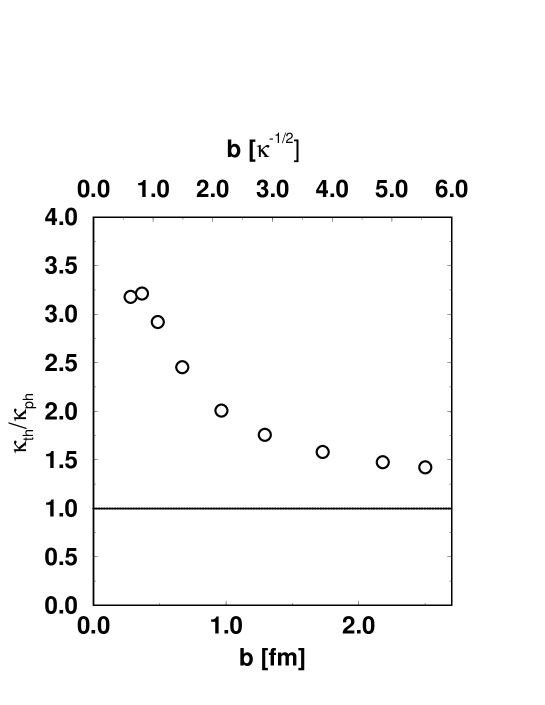
FIG. 5.: The theoretical string tension eq.(44,45,50,51) and numerical data for the full $SU(2)$ string tension $vs.$ $b$.

REFERENCES

- [1] K.G. Wilson, Phys. Rev. D14 (1974) 2455.
- [2] G.’t Hooft, Nucl. Phys. B190 (1981) 455.
- [3] A.A. Abrikosov, JETP 32 (1957) 1442.
- [4] A.S. Kronfeld et al., Phys. Lett. 198B (1987) 516; A.S. Kronfeld, G. Schierholz and U.J. Wiese, Nucl. Phys. B293 (1987) 461.
- [5] T. Suzuki and I. Yotsuyanagi, Phys. Rev. D42 (1990) 4257; Nucl. Phys. B (Proc. Suppl.) 20 (1991) 236; S. Hioki et al., Phys. Lett. B272 (1991) 326 and references therein.
-
[6]
T. Suzuki, Nucl. Phys. B (Proc. Suppl.) 30 (1993) 176;
M. I. Polikarpov, Nucl. Phys. B (Proc. Suppl.) 53 (1997) 134;
G. S. Bali, talk given at 3rd International Conference on Quark Confinement and the Hadron Spectrum (Confinement III), Newport News, VA, June 1998, hep-ph/9809351;
R. W. Haymaker, to be published in Phys. Rept., hep-lat/9809094. - [7] M.N. Chernodub and M.I. Polikarpov, in ”Confinement, Duality and Nonperturbative Aspects of QCD”, p.387, Ed. by Pierre van Baal, Plenum Press, 1998; hep-th/9710205
- [8] A.M. Polyakov, Phys. Lett. B59 (1975) 82.
- [9] T. Banks, R. Myerson and J. Kogut, Nucl. Phys. B129 (1977) 493.
- [10] H. Shiba and T. Suzuki, Phys. Lett. B343 (1995) 315, Phys. Lett. B351 (1995) 519 and references therein.
- [11] A.M. Polyakov, Nucl. Phys. B120 (1977) 429.
-
[12]
G. ’t Hooft, Nucl. Phys. B79 (1974) 276;
A.M. Polyakov, JETP Letters 20 (1974) 194. - [13] R.H. Swendsen, Phys. Rev. Lett. 52 (1984) 1165; Phys. Rev. B30 (1984) 3866,3875.
- [14] J. Smit and A.J. van der Sijs, Nucl. Phys. B355 (1991) 603.
- [15] T.L. Ivanenko and M.I. Polikarpov, preprint ITEP-90-49A (1990).
- [16] P. Becher and H. Joos, Z.Phys. C15 (1982) 343; A.H. Guth, Phys. Rev. D21 (1980) 2291.
- [17] T. Suzuki, Prog. Theor. Phys.80 (1988) 929; S. Maedan and T. Suzuki, Prog. Theor. Phys. 81 (1989) 229.
- [18] M. Baker, J. S. Ball and F. Zachariasen, Phys. Rev. D37 (1988) 1036;Erratum-ibid. D37 (1988) 3785; Phys.Rev. D41 (1990) 2612.
- [19] V. Singh, D. A. Browne and R. W. Haymaker, Phys. Lett. B306 (1993) 115; Nucl. Phys. Proc. Suppl. 30 (1993) 568, hep-lat/9302010; G. S. Bali, C. Schlichter, K. Schilling, talk given at Yukawa International Seminar on Non-Perturbative QCD: Structure of the QCD Vacuum (YKIS 97), Kyoto, Japan, 2-12 Dec 1997, hep-lat/9802005; C. Schlichter, G. S. Bali and K. Schilling, Nucl. Phys. Proc. Suppl. 63 (1998) 519 hep-lat/9709114; M. Baker, N. Brambilla, H. G. Dosch and A. Vairo, Phys. Rev. D58 (1998) 034010.
- [20] S. Kato, S. Kitahara, N. Nakamura and T. Suzuki, Nucl. Phys. B520 (1998) 323.
- [21] H.B. Nielsen and P. Olesen, Nucl. Phys. B 61 (1073) 45.
- [22] Y. Nambu, Proc. Int. Conf. on symmetries and quark models, Detroit, 1969 (Gordon and Breach, New York, 1970) p.269.
- [23] D. Förster, Nucl. Phys. B81 (1974) 84.
- [24] J.L. Gervais and B. Sakita, Nucl. Phys. B91 (1975) 301.
- [25] P. Orland, Nucl. Phys. B428 (1994) 221; M. Sato and S. Yahikozawa, “Topological” Formulation of Effective Vortex Strings, hep-th/9406208.
- [26] Y. Nambu, Phys. Rev. D10 (1974) 4262, Phys. Lett. B80 (1979) 372; A. M. Polyakov, Gauge Fields and Strings, 1987 by Harwood Academic Publishers
- [27] E.T. Akhmedov et al., Phys. Rev. D53 (1996) 2087.
-
[28]
F.V. Gubarev, M.I. Polikarpov and V.I. Zakharov,
Phys. Lett. B438 (1998) 147;
ITEP-TH-73-98, hep-th/9812030. - [29] M.I. Polikarpov, U.J. Wiese and M.A. Zubkov, Phys. Lett. B309 (1993) 133.
- [30] A. M. Polyakov, Nucl. Phys. B268 (1986) 406.
- [31] J. Polchinski and A. Strominger, Phys. Lett. B67 (1991) 1681.
- [32] V.L. Beresinskii, Sov. Phys. JETP 32 (1970) 493.
- [33] J.M. Kosterlitz and D.J. Thouless, J. Phys.,C6 (1973) 1181.
- [34] H.A. Kramers and G.H. Wannier, Phys. Rev. 60 (1941) 252.
- [35] J.V. Jose et al., Phys. Rev. B16 (1977) 1217.
- [36] Y. Munehisa, Phys. Rev. D31 (1985) 1522.
- [37] T.L. Ivanenko, A.V. Pochinskii, M.I. Polikarpov, Phys. Lett. B252 (1990) 631.