Critical Dynamics of the Hybrid Monte Carlo Algorithm

Abstract

We investigate the critical dynamics of the Hybrid Monte Carlo algorithm approaching the chiral limit of standard Wilson fermions. Our observations are based on time series of lengths $O(5000)$ for a variety of observables. The lattice sizes are $16^{3}\times 32$ and $24^{3}\times 40$. We work at $\beta=5.6$, and $\kappa=0.156$, $0.157$, $0.1575$, $0.158$, with $0.83>\frac{m_{\pi}}{m_{\rho}}>0.55$. We find surprisingly small integrated autocorrelation times for local and extended observables. The dynamical critical exponent $z$ of the exponential autocorrelation time is compatible with 2. We estimate the total computational effort to scale between $V^{2}$ and $V^{2\frac{1}{4}}$ towards the chiral limit.

1 INTRODUCTION

Considerable effort has been spent since the early days of exact full QCD simulations with Hybrid Monte Carlo methods [1] to optimize both performance and de-correlation efficiency. The main issues are parameter tuning, algorithmic improvements and assessment of de-correlation.

HMC parameter tuning has been the focus of the early papers. At this time one was restricted to quite small lattices of size $\approx 4^{4}$ [2, 3, 4]. As main outcome, trajectory lengths of $O(1)$ and acceptance rates of $\approx 70$ % have been recommended.

The last three years have seen a series of improvements: Inversion times could be reduced by use of the BiCGstab algorithm [5, 6] and parallel SSOR preconditioning [7]. Together with chronological inversion [8], gain factors between 4 and 8 could be realized [9].

Less research has been done on the critical dynamics of HMC. In Ref. [10], the computer time required to de-correlate a staggered fermion lattice has been estimated to grow like $T\propto m_{q}^{\frac{-21}{4}}$. A similar law has been guessed in Ref. [11] with $T\propto m_{\pi}^{\frac{-23}{2}}$ for two flavours of Wilson fermions. However, so far we lack knowledge about the scaling of the critical behaviour of HMC: a clean determination of the autocorrelation times requires by far more trajectories than feasible at the time. Ref. [14] quotes results in SU(2), the APE group found autocorrelation times in the range of 50 for meson masses [12], the SCRI group gives estimates for $\tau_{int}$ between 9 and 65. However, they seem to behave inconsistently with varying quark mass [13].

SESAM and T$\chi$L have boosted the trajectory samples to $O(5000)$, i. e., by nearly one order of magnitude compared to previous studies [9]. The contiguous trajectories are generated under stable conditions and allow for reliable determinations of autocorrelation times from HMC simulations.

2 AUTOCORRELATION TIMES

The finite time-series approximation to the true autocorrelation function for $A_{t}$, $t=1,\dots,t_{MC}$ is

$$C^{A}(t)=\frac{\sum\limits_{s=1}^{t_{MC}-t}A_{s}A_{s+t}-\frac{1}{t_{MC}-t}\left(\sum\limits_{s=1}^{t_{MC}}A_{s}\right)^{2}}{t_{MC}-t}.$$ (1)

The exponential autocorrelation time is the inverse decay rate of the slowest contributing mode with $\rho^{A}(t)$ being $C^{A}(t)$ normalized to $\rho^{A}(0)=1$, $\tau^{A}_{exp}=\limsup_{t\rightarrow\infty}\frac{t}{-\log\rho^{A}(t)}$. $\tau^{A}_{exp}$ is related to the length of the thermalization phase of the Markov process. To achieve ergodicity the simulation has to safely exceed $\mbox{sup}_{A}\{\tau^{A}_{exp}\}$. The integrated autocorrelation time reads:

$$\tau^{A}_{int}=\frac{1}{2}+\sum_{t^{\prime}=1}^{t_{MC}\to\infty}\rho^{A}(t^{\prime}).$$ (2)

In equilibrium $\tau^{A}_{int}$ characterizes the true statistical error of the observable $A$. The variance $\sigma_{A}^{2}=2\tau^{A}_{int}\sigma^{2}_{0}$ is increased by the factor $2\tau^{A}_{int}$ compared to the result over a sample of $N$ independent configurations. $\tau^{A}_{int}$ is observable dependent.

3 RESULTS

The results given here can only be a small excerpt of our investigation to be presented elsewhere in more detail [15]. The autocorrelation is determined from the plaquette ($\Box_{1\times 1}$) and extended quantities like smeared light meson masses, $m_{\pi}$ and $m_{\rho}$, and smeared spatial Wilson loops ($\Box_{8\times 8}$ and $\Box_{16\times 16}$). They exhibit a large ground state overlap per construction. Furthermore we exploited the inverse of the average number of iterations $\Lambda=N_{kry}^{-1}$ of the Krylov solver which is related to the square root of the ratio of the minimal to the maximal eigenvalue of the fermion matrix [9].

We illustrate the observable dependency of the autocorrelation in Fig. 1.

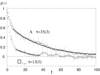
Figure 1: $\rho(t)$ at $\kappa_{\rm sea}=0.157$ for $\Box_{1\times 1}$, and $\Lambda$.

Using $O(3000)$ trajectories we achieve a clear signal for the autocorrelation function. This is the case also for the dynamical samples at $\kappa_{\rm sea}=0.156$, $0.157$ and $0.1575$ as well as on the $24^{3}\times 40$ lattice with $\kappa_{\rm sea}=0.1575$ and $0.158$. $\Lambda$ appears to give an upper estimate to the autocorrelation times of ‘fermionic’ and ‘gluonic’ observables measured.

Shifting the sea-quark mass towards the chiral limit, we observe increasing $\tau_{exp}$ and $\tau_{int}$. Fig. 2 sketches this dependence of $\tau_{int}^{\Lambda}$ on the $16^{3}\times 32$ lattice.

The volume dependence of the autocorrelation was compared for two different lattice sizes at equal $\kappa_{\rm sea}=0.1575$. Unexpectedly, we found $\tau_{exp}$ and $\tau_{int}$, measured in units of trajectory numbers, to decrease by about 50 % for $\Box_{1\times 1}$ and 30 % for $\Lambda$, while switchng from the $16^{3}$ to the $24^{3}$ system. As we chose the length of the HMC molecular dynamics as $T=1$ on the $16^{3}\times 32$ system and $T=0.5$ on the $24^{3}\times 40$ lattice, these numbers are even more surprising. The origin of this phenomenon needs further investigations.

A compilation of $\tau_{exp}$ is given in Fig. 3, the values for $\tau_{int}$ being similar.

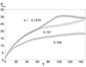
Figure 2: $\kappa_{\rm sea}$ dependency of $\Lambda$ on the $16^{3}\times 32$ lattice.

Figure 3: Exponential autocorrelation times.

The quality of our data allows to address the issue of critical slowing down for HMC. The approach to $\kappa_{\rm sea}^{c}$ amounts to a growing pion correlation length $\xi_{\pi}=1/m_{\pi}a$. The autocorrelation time is expected to scale with a power of $\xi$, $\tau=\epsilon\xi^{z}$. The dynamical critical exponent $z$ governs the scaling of the compute effort, while the knowledge of $\epsilon$ allows to assess its absolute value. Our results are given in Tab. 1.

Table 1: Critical exponents $z$. The $16^{3}\times 32$ results are based on full, the $24^{3}\times 40$ numbers on partial statistics.

Size	$16^{3}\times 32$			$24^{3}\times 40$
Observable	$\Box_{1\times 1}$	$\Lambda$	$\Box_{8\times 8}$	$\Box_{1\times 1}$	$\Lambda$	$\Box_{16\times 16}$
$z_{exp}$	1.8(4)	1.5(4)	1.2(5)	2.2	0.5	0.1
$z_{int}$	1.4(7)	1.3(3)	1.3(3)	2.6	1.0	0.3

For the smaller lattice they tend to be below $z=2$, albeit they are still compatible with 2. It seems that extended observables on the large lattice yield smaller values. However, we have to wait for larger samples to arrive at conclusive answers.

Finally we try to give a conservative guess for the scaling of the compute time $T$ required for de-correlation. The maximal length of $\xi_{\pi}$ has been limited to $V^{\frac{1}{4}}/\xi_{\pi}\approx 4$ in order to avoid finite size effects. With $\xi_{\pi}$ fixed, the volume factor goes as $\xi_{\pi}^{4}$. Furthermore we found $\Lambda\propto\xi^{-2.7}$ for BiCGstab. $z$ lies between 1.3 and 1.8, taking the result from the $16^{3}$ system.

In order to keep the acceptance rate constant, we reduced the time step from 0.01 to 0.004 with increasing lattice size, while we have increased the number of HMC time steps from 100 to 125.

At the same time, as we have already mentioned, the autocorrelation time for the worst case observable $\Lambda$ went down by 30 % compensating the increase in acceptance rate cost! In a conservative estimate, we thus would assume that the total time $T$ scales as $\xi_{\pi}^{8}$ to $\xi_{\pi}^{8.5}$. This guess translates to $T\propto V^{2}$ - $V^{2.2}$.

4 SUMMARY

The autocorrelation times from HMC under realistic conditions are smaller than anticipated previously, staying below the value of $60$ trajectories for $\tau_{exp}$. $z$ is compatible with 2. The computer time to generate decorrelated configurations scales according to $V^{2}$, a very encouraging result compared to previous estimates [10, 11].

References

- [1] S. Duane, A. Kennedy, B. Pendleton and D. Roweth, Phys. Lett. B 195 (1987) 216.
- [2] M. Creutz, in: Proc. of Peniscola 1989, Nuclear Equation of State, pp. 1-16.
- [3] R. Gupta, G. W. Kilcup, S. R. Sharpe, Phys. Rev. D 38 (1988) 1278.
- [4] K. Bitar et al., Nucl. Phys. B 313 (1989) 377.
- [5] A. Frommer et al., IJMP C5 (1994) 1073.
- [6] Ph. de Forcrand, Nucl. Phys. B (Proc. Suppl.) 47 (1996) 228-235.
- [7] S. Fischer et al.: Comp. Phys. Comm. 98 (1996) 20-34.
- [8] R. C. Brower, T. Ivanenko, A. R. Levi, K. N. Orginos, Nucl. Phys. B 484 (1997) 353-374.
- [9] Th. Lippert et al., hep-lat/9707004, to appear in Nucl. Phys. B (Proc. Suppl.).
- [10] S. Gupta, A. Irbäck, F. Karsch and B. Petersson, Phys. Lett. 242B (1990) 437.
- [11] R. Gupta, et al., Phys. Rev. D 44 (1991) 3272.
- [12] S. Antonelli et al., Nucl. Phys. B (Proc. Suppl.) 42 (1995) 300-302.
- [13] K.M. Bitar et al., Nucl. Phys. B (Proc. Suppl.) 53 (1997) 225-227.
- [14] K. Jansen, C. Liu, Nucl. Phys. B 453 ((1995)) 375.
- [15] SESAM and TL-collaboration, to appear.
- [16] G. Boyd et al., Nucl. Phys. B (Proc. Suppl.) 53 (1997) 544.