A Coupled-Cluster Formulation of Hamiltonian Lattice Field Theory: The Non-Linear Sigma Model

Abstract

We apply the coupled cluster method (CCM) to the Hamiltonian version of the latticised $O(4)$ non-linear sigma model. The method, which was initially developed for the accurate description of quantum many-body systems, gives rise to two distinct approximation schemes. These approaches are compared with each other as well as with some other Hamiltonian approaches. Our study of both the ground state and collective excitations leads to indications of a possible chiral phase transition as the lattice spacing is varied.

Contents

1 Introduction; 2 The $O(4)$ non-linear sigma model; 3 Elements of coupled cluster theory; 3.1 The standard form of the CCM; 3.2 The functional form of the CCM; 4 The operatorial form of the CCM for classical spin models; 4.1 The LSUB2 approximation; 4.2 The SUB2-$n$ approximations; 4.3 Full SUB2 calculations; 4.4 Collective excitations; 5 The functional form of the CCM for classical spin models; 5.1 The LSUB2 aproximation; 5.2 The SUB2-$n$-$m$ approximations; 5.3 Collective excitations; 6 Solution and Results; 6.1 Numerical methods; 6.2 LSUB2 Results; 6.3 SUB2-$n$(-$m$) Results; 6.4 Excitations; 6.5 Comparison with other work; 7 Conclusions and outlook; A Quantisation; B Gegenbauer polynomials

1 Introduction

The physics of particles interacting through the strong forces at low energies is dominated by pions (see, e.g., the discussion in Ref. [1]). In the hadronic sector the exchange of single and correlated pions between nucleons determines the long-range and intermediate-range behaviour of the nuclear force. The QCD Lagrangian, which is supposed to govern all strong interaction physics, has a chiral symmetry. Were this symmetry realised in nature, we would expect all hadrons to come in chiral pairs in which each hadron has a partner of the same mass but opposite parity. The fact that this does not actually occur is due to the effect of spontaneous breaking of the chiral symmetry which arises from the development of a condensate of quarks and gluons. The pions are interpreted as the Goldstone bosons which occur in such a scenario. If QCD were exactly chirally symmetric we would expect to find them at zero mass. The fact that their rest-mass is about 140 MeV/c² is due to the effect of the small masses carried by the quarks. This can be expressed in the Gell-Mann-Oakes-Renner relation [2], which relates the pion mass to the quark condensate and to the up and down quark masses, $m_{u}$ and $m_{d}$ respectively,

$$m_{\pi}^{2}=-\left(\frac{2}{f_{\pi}}\right)\langle\bar{\psi}\psi\rangle(m_{u}+m_{d}).$$ (1)

Here $\langle\bar{\psi}\psi\rangle$ is the quark condensate in vacuum.

In recent years a simple scaling argument by Brown and Rho [3] has sparked heated discussions about how mesons behave in a medium, where the quark condensate changes due to a partial restoration of chiral symmetry. The same question can be asked for finite temperature. One believes that for temperatures of around the order of the pion mass the chiral condensate will disappear and chiral symmetry will be restored [4]. It is believed that in heavy ion collisions it is possible to inject enough energy to create such a phase. It is not yet clear whether such a plasma can reach thermal equilibrium, nor whether the time scale is long enough for the chiral phase to develop.

All these issues have renewed interest in the dynamics of systems of pions. At the same time a revival has occurred in so-called baryon chiral perturbation theory [5], where the most general effective Lagrangian compatible with chiral symmetry is constructed, and all constants are fitted to experiments. This approach, which has met great success in the meson sector [1], is now actively being pursued in the baryonic sector.

As mentioned above, pions find their origin in the chiral symmetry, which can be related to the fundamental QCD Lagrangian. In the dynamical breaking of the symmetry the chiral partners of hadrons disappear and a set of three massless bosons, the Goldstone bosons, emerges. Although the mechanism is well understood, it is difficult to see explicitly how pions arise from the original QCD Lagrangian, especially since the pions are known to be composite particles. Therefore one often works with an effective Lagrangian which is compatible with the consequences of spontaneous symmetry breaking. The pion dynamics is somewhat restricted, since we have partial conservation of the axial current (PCAC), which limits the interactions we can build into our models. One model that satisfies these constraints is the $O(4)$ non-linear sigma model, which we shall study in this paper.

The class of non-linear sigma models plays an illustrative rôle in many physical phenomena [6, 7]. In particular, the $O(4)$ version of the model can be used to describe the dynamics of pions. In that case the $O(4)$ symmetry can be broken explicitly, but the isospin $O(3)$ sub-symmetry must be retained. Using a perturbative approach for the model in 2 dimensions (1 space and 1 time) one finds that it exhibits both infrared and ultraviolet divergences [6]. The latter are thought to be responsible for dimensional transmutation, the process whereby the dimensionless coupling constant acquires a dependence on a fundamental length, such as the QCD scale in QCD.

The short-distance behaviour has to be regularised, which is generally done by putting the model onto a lattice. For some finite lattice spacing one expects a phase transition between a system with essentially free rotators which interact weakly (at large lattice spacings), and a system of tightly bound rotators which exhibit only collective behaviour (at small lattice spacings). In the former phase all excitations are massive and are characterised by the quantum numbers of the free rotator. In the latter case the excitation energy gap disappears. However, for two dimensions (one space and one time) the situation is different. From exact results it is known that the phase transition disappears due to strong interactions among the Goldstone bosons [6]. The excitations remain massive, although their masses decrease with decreasing lattice spacing. This result is confirmed in dimensional regularisation [8], as is the asymptotic freedom of the two-dimensional non-linear sigma model.

Most results in $O(4)$ theory have been derived in a Euclidean framework [9]. In that case there is also a clear correspondence with high-temperature spin models [10]. In a Euclidean framework space and time are treated on an equal footing. Not only is the time coordinate discretised but it is also taken to be imaginary. Apart from the ground-state energy it is very hard to recover properties of the system, and it is not clear whether the Euclidean and the Minkowskian (or Hamiltonian) methods yield the same result in a non-perturbative framework, especially since the lattice regularisation is implemented in such different ways in the two methods.

In a Hamiltonian framework time is taken to be real and continuous (as it is in nature). One can construct quantum-mechanical (Schrödinger) states and calculate basic expectation values. However, for gauge theories the gauge has to be fixed when constructing a Hamiltonian, and therefore gauge invariance might be destroyed in subsequent approximations. Space is discretised on a lattice, and the lattice spacing is the only dimensional parameter in the model. The phase transition from the disoriented (symmetric) phase of free rotators to the oriented (spontaneously broken symmetry) phase of tightly bound rotators can be seen as the dimensional transmutation, which sets the scale at which the system starts to exhibit the basic continuum behaviour.

As the non-linear sigma model is an effective field theory for pions these features should put pion dynamics in a broader context. Indeed, we see that in low-energy pion dynamics the interaction vanishes as the momenta go to zero, which follows rather naturally from the fact that the pions are the Goldstone bosons of the chiral symmetry and the interaction is dictated by the spontaneous symmetry-breaking mechanism. However, since the pion is a composite particle the connection should break down for higher momenta (preferably somewhere near the QCD scale). This makes it difficult to connect excitations in the large lattice spacing systems we are investigating to actual physical particles. The system is more closely related to the dynamics of rotators described above.

Apart from its intrinsic physical interest the non-linear sigma model is an ideal testing ground for non-perturbative methods. Although the Lagrangian is fairly simple and the degrees of freedom are restricted, it still has the richness of a full physical theory, whose properties should be correctly described by a proper non-perturbative method for the study of lattice field theories. The structure of field theories on the lattice is such that it begs to be treated by many-body techniques which first allow the ground state to be approximated in a well-determined and controlled way. Recently, Chin [11] has performed such a many-body calculation for the model being studied in this paper, using a variational technique embedded in a more general correlated basis function (CBF) approach. By contrast with the techniques used here, the CBF method, which uses a generalized Jastrow-correlated wave function cannot easily be formulated as a set of algebraic equations. Instead, it needs to be solved by Monte Carlo techniques on a finite portion of the infinite lattice, just as in most lattice-gauge approaches. The limit to an infinite lattice needs to be taken at the end of the calculation, using heuristic or theoretical scaling arguments.

Our approach to the problem is the so-called coupled cluster method (CCM). The CCM is now widely acknowledged to provide one of the most widely applicable and most powerful of all microscopic formulations of quantum many-body theory. In the many applications which have so far been made in such diverse fields as nuclear physics, quantum field theory, condensed matter physics, quantum magnetism, and quantum chemistry [12], the CCM has been found to provide results which are among the most accurate available. Indeed, it has been shown to give results comparable to those from large-scale quantum Monte Carlo calculations in those cases where the latter can be performed. The interested reader is referred to Ref. [12] for a survey of the method and an overview of its applications.

The CCM is formulated in terms of cluster correlation functions. These correlation functions, although typically only correlating the particles (or spins, or fields) on clusters of lattice sites with a finite spatial extent, do nevertheless extend the correlated wave function over the infinite lattice. In the CCM, unlike in CBF and most other lattice calculations, the lattice may be treated as infinite from the outset, as we will see below.

In particular, the CCM has recently been applied to simple $U(1)$ lattice gauge field theory [13, 14], and has been shown to provide an interesting scheme for studying the properties of such models. In the current work we introduce a variant of the CCM that works with functions rather than with the more usual operators. This approach will be discussed in considerable detail in the present paper, although we shall succeed in constructing an operatorial approach as well.

The remainder of this paper is organised as follows. In Sec. 2 we briefly discuss the $O(4)$ non-linear sigma model and the Hamiltonian we construct from it (with some details relegated to Appendix A). Then, in Sec. 3, we shall succinctly introduce the traditional form of the CCM and, in some more detail, the functional form. In Sec. 4 we lay the theoretical framework for an investigation of the $O(4)$ non-linear sigma model using the traditional CCM approach. The same is done in Sec. 5 for the functional method. In Sec. 6 we collect the results from the various schemes, and contrast these both among themselves and with the few other results available. Finally we give a summary and outlook in Sec. 7.

2 The $O(4)$ non-linear sigma model

The $O(4)$ non-linear sigma model is defined by the Lagrangian density

$${\mathcal{L}}=\frac{1}{4}\mathrm{Tr}(\partial_{\mu}U\partial^{\mu}U^{\dagger}),$$ (2)

where $U$ is an $SU(2)$ matrix-valued field of $2\times 2$ unitary matrices, which is often conveniently represented by a sum of unit and Pauli matrices,

$$U=n_{4}I+i\mathbf{\tau}\cdot\mathbf{n},$$ (3)

and the unitarity constrains the four-vector $\hat{n}=(\mathbf{n},n_{4})$ to have unit length.

We shall study the model on a spatial grid which is a cubic lattice in three dimensions and with continuous time, in a Hamiltonian formalism. We replace the spatial derivatives by finite differences, with a lattice spacing $a$. Since the time-derivative part of the Lagrangian describes a freely rotating four-vector constrained to the unit sphere, it is not implausible that the kinetic energy in the Hamiltonian form at each point in space can be reduced to the angular part of the Laplacian, as is shown in Appendix A. Another way to represent this result is

$$H = \mbox{$\frac{1}{2}$}\sum_{\mathbf{i}}\mathbf{I}_{\mathbf{i}}^{2}+\frac{1}{4a^{2}}\sum_{\langle\mathbf{i}\mathbf{j}\rangle}\mathrm{Tr}((U_{\mathbf{i}}-U_{\mathbf{j}})(U^{\dagger}_{\mathbf{i}}-U^{\dagger}_{\mathbf{j}}))$$ (4)

$$= \mbox{$\frac{1}{2}$}\sum_{\mathbf{i}}\mathbf{I}_{\mathbf{i}}^{2}+\frac{1}{a^{2}}\sum_{\langle\mathbf{i}\mathbf{j}\rangle}\left[1-\cos(\theta_{\mathbf{i}\mathbf{j}})\right].$$

The lattice Hamiltonian contains a trivial factor $a^{D}$: the volume of the unit lattice cell in $D$ spatial dimensions. We implicitly assume that all expectation values scale with this volume. Here $I_{a}$ can be taken as either the left or right SU(2) generators,

$$[{I}_{a\mathbf{i}},U_{\mathbf{j}}]=i\tau_{a}U_{\mathbf{i}}\delta_{\mathbf{i}\mathbf{j}}\qquad{\rm or}\qquad[{I}_{a\mathbf{i}},U_{\mathbf{j}}]=iU_{\mathbf{i}}\delta_{\mathbf{i}\mathbf{j}}\tau_{a},$$ (5)

and $\theta_{\mathbf{i}\mathbf{j}}\equiv\hat{n}_{\mathbf{i}}\cdot\hat{n}_{\mathbf{j}}$ is the angle between the two unit vectors $\hat{n}_{\mathbf{i}}$ and $\hat{n}_{\mathbf{j}}$ describing $U_{\mathbf{i}}$ and $U_{\mathbf{j}}$. We use here the convention related to the $O(4)$ symmetry. Factors of a half might appear in other conventions related to the isospin symmetry (and see, e.g., Chin [11]). We note that these different conventions will also lead to corresponding alternative definitions of the kinetic energy. We ourselves choose the convention which yields the kinetic energy of a unit mass on the four-dimensional unit sphere. Relabelling $\lambda=\frac{1}{a^{2}}$, we have the classical spin model

$$H=\mbox{$\frac{1}{2}$}\sum_{\mathbf{i}}\mathbf{I}_{\mathbf{i}}^{2}+\lambda\sum_{\langle\mathbf{i}\mathbf{j}\rangle}(1-\cos\theta_{\mathbf{i}\mathbf{j}}),$$ (6)

where the sum over $\langle\mathbf{i}\mathbf{j}\rangle$ runs over all nearest-neighbour pairs, and counts each pair (or lattice link) only once.

The Hamiltonian can thus be interpreted as that of freely rotating unit vectors (or quantum rotors), with a nearest-neighbour coupling that tends to align them. It is this competition between free rotation and an alignment force that makes these models interesting to study. It also shows that they are identical to classical spin systems on a lattice, which can be obtained as either the large-$J$ limit of a finite-$J$ lattice spin model, or in the calculation of the partition function of a classical lattice spin problem.

3 Elements of coupled cluster theory

We start with an $O(N)$ Hamiltonian of the form

$$H=\sum_{\mathbf{i}}K_{\mathbf{i}}+\lambda\sum_{\langle\mathbf{i}\mathbf{j}\rangle}(1-\hat{n}_{\mathbf{i}}\cdot\hat{n}_{\mathbf{j}}).$$ (7)

Here $K_{\mathbf{i}}$ is the kinetic energy on the $N$-dimensional unit sphere at lattice point $\mathbf{i}$. The eigenstates of $K_{\mathbf{i}}$ are the (hyper)spherical harmonics $\left|J\alpha\right\rangle_{\mathbf{i}}$,

$$K_{\mathbf{i}}\left|J\alpha\right\rangle_{\mathbf{i}}=\epsilon_{J}\left|J\alpha\right\rangle_{\mathbf{i}}.$$ (8)

Here we have divided the quantum numbers into those $(J)$ that determine the eigenvalues of $K_{\mathbf{i}}$, and those $(\alpha)$ that label the different degenerate eigenstates.

There are now at least two distinct ways to formulate a coupled-cluster approach for such a classical spin model. Firstly, there is an operatorial approach, which models itself closely on the standard formulation of the CCM, albeit with rather artificial operators. Secondly, there also exists a functional approach, which was first applied to lattice QED problems. Although the latter functional approach appears to be more natural for the present study, both methods are investigated and compared below.

3.1 The standard form of the CCM

Coupled cluster theory is one of the mainstays of modern microscopic quantum many-body theory, and reviews of the method are available (and see, e.g., ref. [12]). We shall therefore only give a very short summary of the salient points of the method; for full details see Ref. [12] and references cited therein.

The key feature of coupled cluster theory is its construction of a systematically improvable approximation to the exact correlated ground state of an interacting system, by the action of the exponential of an operator $\hat{S}$ on some suitable model state or bare vacuum, $|0\rangle$, which may (but does not have to) be chosen as the exact ground state in some limit. No attempt is made to normalise this state against itself, but one rather constructs a bra state in a bi-orthogonal system such that the inner product of the bra and the ket states remains unity. One starts from a set of (generalized) multi-particle or multi-mode creation operators $a^{\dagger}_{n}$, where the corresponding hermitian conjugate annihilation operators destroy the vacuum, $a_{n}|0\rangle=0$. We now write the correlated ground state as

$$\left|\Psi\right\rangle=\exp\left(\sum_{n}S_{n}a^{\dagger}_{n}\right)\left|0\right\rangle.$$ (9)

This state satisfies an intermediate normalisation condition, $\left\langle 0|\Psi\right\rangle=1$. In many-body applications, the exponential Ansatz of Eq. (9) guarantees proper size-extensivity and conformity with the Goldstone linked-cluster theorem even when approximations are made. By contrast, the corresponding linear parametrisation which characterises the corresponding configuration-interaction method (or generalized many-body shell model) will not, in general, obey either of these important properties when approximations are made. One also parameterises the corresponding correlated bra state as

$$\left\langle\smash[t]{\tilde{\Psi}}\right|=\left\langle 0\right|\left(1+\sum_{n}\tilde{S}_{n}a_{n}\right)\exp\left(-\sum_{n}S_{n}a^{\dagger}_{n}\right),$$ (10)

where the coefficients $S_{n}$ and $\tilde{S}_{n}$ are to be determined independently by an extremum requirement, which can be given the variational form

$$\delta(I[S,\tilde{S}])=0,$$ (11)

with

$$I[S,\tilde{S}]=\left\langle\smash[t]{\tilde{\Psi}}\right|H\left|\Psi\right\rangle,$$ (12)

where $I[S,\tilde{S}]$ is the functional with respect to the infinite set of coefficients $S=\{S_{n}\ |\ n=1,2,\cdots\}$ and $\tilde{S}=\{\tilde{S}_{n}\ |\ n=1,2,\cdots\}$. In practice, however, we need to truncate the sum over creation and annihilation operators, and a consistent truncation scheme is found by restricting the two sets of coefficients in the same manner. For this choice we also find that the Hellmann-Feynman theorem is satisfied, i.e.

$$\left\langle\smash[t]{\tilde{\Psi}}\right|\partial_{\lambda}H\left|\Psi\right\rangle=\partial_{\lambda}E,$$ (13)

where $E$ is the ground-state energy, $E\equiv\left\langle\smash[t]{\tilde{\Psi}}\right|H\left|\Psi\right\rangle$. Finally, in a formulation of the theory where the coefficients $S_{n}$ and $\tilde{S}_{n}$ are time-dependent, we find that $S_{n}$ and $\tilde{S}_{n}$ are canonically conjugate variables. There is a deep connection between these three properties, and we cannot give up one without giving up something else as well  [12]. In particular we note that although in untruncated, and hence exact, parametrisations of the form of Eqs. (9) and (10), the hermiticity relation $\tilde{\left|\Psi\right\rangle}=\left|\Psi\right\rangle/\langle\Psi|\Psi\rangle$ would hold, when Eqs. (9) and (10) are truncated this exact hermiticity is broken in general. Although Arponen [15] has discussed means to restore the hermiticity within the CCM formalism, we do not pursue this point further here.

3.2 The functional form of the CCM

The functional form is similar to the method sketched above, and as far as we are aware has first been used in refs. [13, 14]. The key ingredient is the parametrisation of the ground-state ket wave function in the exponential form

$$\left\langle\{r\}|\Psi\right\rangle=\exp\left[S(\{r\})\right],$$ (14)

where $\left|\{r\}\right\rangle$ is some suitably chosen complete set of wave functions. Such an approach appears to be naturally suited to lattice Hamiltonians, where a complete set of functions can often be chosen to be the product of complete sets at each lattice site. Truncations, which in the operator form are performed on the number and type of creation operators, are now performed on the functional dependence of the function $S(\{r\})$, typically by expansion in a complete set of appropriate functions. Once we construct the mode of action of the Hamiltonian on functions of the variables ${\{r\}}$ – typically a differential, but at worst an integro-differential, operator – we can proceed as before and use the respective bra-state parametrisation,

$$\left\langle\smash[t]{\tilde{\Psi}}|\{r\}\right\rangle=[1+\tilde{S}(\{r\})]\exp\left[-S(\{r\})\right],$$ (15)

and a variational functional $I[S,\tilde{S}]$ defined by

$$I[S,\tilde{S}]=\int d\{r\}d\{r^{\prime}\}[1+\tilde{S}(\{r\})]\exp\left[-S(\{r\})\right]\left\langle\{r\}\right|H\left|\{r^{\prime}\}\right\rangle\exp\left[S(\{r^{\prime}\})\right].$$ (16)

One typically excludes a constant term from $S$ and $\tilde{S}$ (corresponding to the exclusion of the identity operator from the sum over the multi-configurational creation operators in the various terms in Eqs. (9) and (10)). However, we now no longer have intermediate normalisation. Thus, the constant part of $\exp\left(S(\{r\})\right)$ is not one, since an arbitrary power of a function orthogonal to the constant function can contain a constant part. In this case we need to enquire what happens with the Hellmann-Feynman theorem and the canonical variables in the time-dependent formalism? The key to the answer lies in orthogonality. While this is provided for by Wick’s theorem when using the operator form, in the functional form this requires an expansion in orthogonal functions, relative to (typically) a product of integrations. This will be shown to be straightforwardly implementable in the lowest set of approximations (SUB2-$n$, where only $n$ two-body correlations are retained) for the model under consideration here. Since many-body orthogonal polynomials are not straightforward to define, more complicated correlations involving more than pairwise correlations do not seem to be easy to formulate in the functional form of the theory. It may still be that for certain classes of lattice models a functional form is easier to use, and even though we lose some of the elegance of the standard CCM, we might nevertheless still be able to proceed using this method.

4 The operatorial form of the CCM for classical spin models

Let us first investigate the operatorial CCM approach when applied to classical spin models of the form given in Eq. (7). We use the fact that the uncorrelated ground-state wave function is given by the constant function (the product over the grid of the lowest eigenstates $\left|0\right\rangle_{\mathbf{i}}$ of the kinetic energy operator $K_{\mathbf{i}}$). We now define a set of excitation operators for the CCM by

$$C^{\dagger}_{\mathbf{i}J\alpha}=\left|J\alpha\right\rangle_{\mathbf{i}}\left\langle 0\right|_{\mathbf{i}}\ ;\ \ J>0,$$ (17)

which are chosen such that their hermitian conjugates annihilate the vacuum. The quantum number $J$ labels the energy eigenstates of a single rotor, and $\alpha$ labels the different states for a given energy. We shall use the notation

$$\left|{\left\{\hat{n}\right\}}\right\rangle=\prod_{\mathbf{i}}\left|\hat{n}_{\mathbf{i}}\right\rangle,\;\;\;\left|{\left\{0\right\}}\right\rangle=\prod_{\mathbf{i}}\left|0_{\mathbf{i}}\right\rangle,$$ (18)

where the states $\left|\hat{n}_{\mathbf{i}}\right\rangle$ are the standard coordinate representation at lattice site $\mathbf{i}$. We shall mainly be concerned with the SUB2 family of approximations, in which only correlations between pairs of spins are incorporated, and in which the coupled cluster operator can hence be written as

$$\hat{S}_{2}\equiv\sum_{[\mathbf{i}\mathbf{j}]}\hat{S}_{2\mathbf{i}\mathbf{j}}=\sum_{I[\mathbf{i}\mathbf{j}]}s_{I}\left[C^{\dagger}_{\mathbf{i}I}\otimes C^{\dagger}_{\mathbf{j}I}\right]^{(0)},$$ (19)

where $I$ is now the label for the energy eigenstates in the relative angle between the spins at lattice sites $\mathbf{i}$ and $\mathbf{j}$. The sum over $[\mathbf{i}\mathbf{j}]$ is over all pairs of lattice sites, $\mathbf{i}$ and $\mathbf{j}$, counting each pair once, by contrast with the sum $\langle\mathbf{i}\mathbf{j}\rangle$ which runs over the nearest-neighbour pairs only, and which we introduced previously in Eq. (6). We have suppressed the $\alpha$ labels, because these are implicitly summed over in the scalar coupling. Since the only scalar that we can construct from the two vectors $\hat{n}_{\mathbf{i}}$ and $\hat{n}_{\mathbf{j}}$ is their inner product, we find

$$\left\langle\hat{n}_{\mathbf{i}},\hat{n}_{\mathbf{j}}\right|\hat{S}_{2\mathbf{i}\mathbf{j}}\left|0_{\mathbf{i}},0_{\mathbf{j}}\right\rangle = \frac{1}{\sqrt{\Omega_{N}}}S_{2}(\hat{n}_{\mathbf{i}}\cdot\hat{n}_{\mathbf{j}})=\frac{1}{\sqrt{\Omega_{N}}}S_{2}\left(\cos\theta_{\mathbf{i}\mathbf{j}}\right);$$ (20)

$$\hat{S}_{2\mathbf{i}\mathbf{j}} = \int d\hat{n}_{\mathbf{i}}d\hat{n}_{\mathbf{j}}|{\hat{n}_{\mathbf{i}},\hat{n}_{\mathbf{j}}}\rangle\,\frac{1}{\sqrt{\Omega_{N}}}S_{2}(\cos\theta_{\mathbf{i}\mathbf{j}})\,\langle{0_{\mathbf{i}},0_{\mathbf{j}}}|,$$ (21)

where $\Omega_{N}$ is the surface of the $N$-dimensional unit sphere. The potential can be expressed in the same way. Since the potential only depends on the relative angle between nearest-neighbour spins we require only the scalar coupling of spins

$$\hat{V}_{\mathbf{i}\mathbf{j}}=\int d\hat{n}_{\mathbf{i}}d\hat{n}_{\mathbf{j}}|{\hat{n}_{\mathbf{i}},\hat{n}_{\mathbf{j}}}\rangle\,\lambda\,(1-\cos\theta_{\mathbf{i}\mathbf{j}})\,\langle{\hat{n}_{\mathbf{i}},\hat{n}_{\mathbf{j}}}|.$$ (22)

We now deal with the operators $\hat{S}_{2}$. The best way to calculate the expectation value of the variational functional

$$I[S,\tilde{S}]=\left\langle{\left\{0\right\}}\right|(1+\hat{\tilde{S}})e^{-\hat{S}}He^{\hat{S}}\left|{\left\{0\right\}}\right\rangle,$$ (23)

is to use the usual nested commutator approach to the CCM,

$$e^{-\hat{S}}He^{\hat{S}}=H+[H,\hat{S}]+\frac{1}{2}[[H,\hat{S}],\hat{S}]+\ldots,$$ (24)

which truncates at second order for the current Hamiltonian since the Hamiltonian in this form is a second order differential operator which can act only at one or two factors in the ket state. We then evaluate the ensuing expectation values by introducing complete states of intermediate states at both sides of $H$.

We use completeness in the form

$$\left|{\left\{\hat{m}\right\}}\right\rangle=\int d\mu({\left\{\hat{n}\right\}})\left|{\left\{\hat{n}\right\}}\right\rangle\left\langle{\left\{\hat{n}\right\}}|{\left\{\hat{m}\right\}}\right\rangle,$$ (25)

where $\int d\mu({\left\{\hat{n}\right\}})$ describes the product, over the whole lattice, of integrals over the $N$-dimensional unit sphere appropriate to the general $O(N)$ case. Relation (25) assumes the overlap

$$\left\langle\hat{n}_{\mathbf{i}}|\hat{m}_{\mathbf{i}}\right\rangle=\delta(\hat{n}_{\mathbf{i}}-\hat{m}_{\mathbf{i}}).$$ (26)

Using the fact that the operator $\hat{S}_{\mathbf{i}\mathbf{j}}$, where we now and henceforth suppress the pairwise subscript 2, projects to the right onto the ground state for sites $\mathbf{i},\mathbf{j}$, we find that the only parts of the commutators in Eq. (24) that contribute are these where all $\hat{S}$ operators are to the right of the Hamiltonian.

Using the fact, as follows from normalisation, that

$$\left\langle\hat{n}_{\mathbf{i}}|0_{\mathbf{i}}\right\rangle=\sqrt{\frac{1}{\Omega_{N}}},$$ (27)

where $\Omega_{N}$ is the surface area of the $N$-dimensional unit sphere, i.e., $\Omega_{4}=2\pi^{2}$ for $O(4)$, we get

$$I[S,\tilde{S}]=\int d\mu({\left\{\hat{n}\right\}})\int d\mu(\{\hat{n}^{\prime}\})\left\langle{\left\{0\right\}}\right|1+\hat{\tilde{S}}\left|{\left\{\hat{n}\right\}}\right\rangle\left\langle{\left\{\hat{n}\right\}}\right|H|\{\hat{n}^{\prime}\}\rangle\langle\{\hat{n}^{\prime}\}|(1+\hat{S}+\frac{1}{2}\hat{S}^{2})\left|0\right\rangle.$$ (28)

If $N_{g}$ is the number of lattice (or grid) points, we may now write

$$\left\langle{\left\{\hat{n}\right\}}\right|{\hat{S}}\left|{\left\{0\right\}}\right\rangle=\left({\Omega_{N}}\right)^{-N_{g}/2}\sum_{[\mathbf{i}\mathbf{j}]}S_{{\chi_{\mathbf{i}-\mathbf{j}}}}(\hat{n}_{\mathbf{i}}\cdot\hat{n}_{\mathbf{j}}),$$ (29)

and

$$\left\langle{\left\{\hat{n}\right\}}\right|{\hat{S}}^{2}\left|{\left\{0\right\}}\right\rangle=\left({\Omega_{N}}\right)^{-N_{g}/2}\sideset{}{{}^{\prime}}{\sum}_{[\mathbf{i}\mathbf{j}],[\mathbf{i}^{\prime}\mathbf{j}^{\prime}]}S_{{\chi_{\mathbf{i}-\mathbf{j}}}}(\hat{n}_{\mathbf{i}}\cdot\hat{n}_{\mathbf{j}})S_{{\chi_{\mathbf{i}^{\prime}-\mathbf{j}^{\prime}}}}(\hat{n}_{\mathbf{i}^{\prime}}\cdot\hat{n}_{\mathbf{j}^{\prime}})$$ (30)

where the prime on the sum means that only totally disconnected diagrams are allowed, due to the projective properties of our creation operators. The notation ${\chi_{\mathbf{i}-\mathbf{j}}}$ denotes an integer irrep label; it indicates that we assume that $\hat{S}$ is invariant under symmetries of the lattice, and we have to identify components at symmetry-equivalent lattice sites. Finally

$$\left\langle{\left\{0\right\}}\right|1+\hat{\tilde{S}}\left|{\left\{\hat{n}\right\}}\right\rangle=\left({\Omega_{N}}\right)^{-N_{g}/2}\left(1+\sum_{[\mathbf{i}\mathbf{j}]}{\tilde{S}}_{{\chi_{\mathbf{i}-\mathbf{j}}}}(\hat{n}_{\mathbf{i}}\cdot\hat{n}_{\mathbf{j}})\right).$$ (31)

In a SUB2-type approximation (i.e., when the correlation operators $\hat{\tilde{S}}$ and $\hat{S}$ are two-body operators), we can use those parts of the Hamiltonian where only the relative variables, $\theta_{\mathbf{i}\mathbf{j}}$ defined by $\cos\theta_{\mathbf{i}\mathbf{j}}=\hat{n}_{\mathbf{i}}\cdot\hat{n}_{\mathbf{j}}$, are present

$$H\to\sum_{[\mathbf{i}\mathbf{j}]}\frac{-1}{\sin^{2}(\theta_{\mathbf{i}\mathbf{j}})}\partial_{\theta_{\mathbf{i}\mathbf{j}}}(\sin^{2}\theta_{\mathbf{i}\mathbf{j}}\partial_{\theta_{\mathbf{i}\mathbf{j}}})+\sum_{\langle\mathbf{i}\mathbf{j}\rangle}\lambda[1-\cos\theta_{\mathbf{i}\mathbf{j}}].$$ (32)

where the kinetic operator $K$ acts twice on each relative angle $\theta_{\mathbf{i}\mathbf{j}}$: one from each lattice site, $K_{\mathbf{i}}$ and $K_{\mathbf{j}}$. This explains the factor of two in the kinetic energy terms in Eq. (32) with respect to those in the original Hamiltonian defined in Eq. (6).

Figure 1: The basic building blocks for the diagrammatic analysis of the functional $I$. We denote $S$ by a thin solid line, $\tilde{S}$ by a thick solid line and the potential by a dashed line. A cross denotes the action of the kinetic energy operator. Open circles indicate that the coordinates at these lattice points are not integrated over.

The part of the integration measure over the 4-sphere dependent on $\theta$ is $\sin^{2}\theta\,d\theta$. Integrating over a single $S_{n}$ is the projection onto the model state, which is by construction zero. Using this fact, we get the sum of all possible connected diagrams, generated from the basic ones sketched in Fig. 1. The key idea is to construct all diagrams for $I[\tilde{S},S]$ on the lattice that can be made from drawing any of the lines ($S$, $\tilde{S}$, $V$) between the lattice points, subject to the condition that the diagram is closed, no two functions $S$ can connect at the same point, and the potential connects only nearest neighbours. Diagrams that do not contain a potential must contain one kinetic energy operator $K$, and they can contain at most one line $\tilde{S}$.

In the so-called LSUB2 approximation we retain only nearest-neighbour pairwise correlations. In Fig. 2 we place the diagrams on a lattice. Since the ket-state CCM equations are obtained through variation of $I[S,\tilde{S}]$ with respect to $\tilde{S}_{\mathbf{i}\mathbf{j}}$, we should not integrate over the unit vector at these grid points. This is denoted by the open circles in the CCM equation. For fixed position of the $\tilde{S}$ line, the square diagram in $I$ can be produced in various ways. We choose to pick one orientation, and give it a weight $\alpha^{11}_{1}$ labelling the number of equivalent diagrams. The square diagram is the only non-local diagram in $I$, i.e., it involves nontrivial integrations over additional lattice sites, other than $\mathbf{i}$ and $\mathbf{j}$ from the variation with respect to $\tilde{S}_{\mathbf{i}\mathbf{j}}$.

Figure 2: The diagrams for the LSUB2 approximation, together with the non-linear equation for $S$ and the equation for the energy.

Of course both the action and the energy are infinite for an infinite lattice. It is clear, in the LSUB2 approximation, that when the terms proportional to $\tilde{S}$ vanish, which happens after minimisation, the energy can be expressed as a sum over all nearest-neighbour links of the three diagrams shown in the last line of Fig. 2 which do not contain a thick line. Using the standard assumption that each of these diagrams is independent of the (nearest-neighbour) sites $\mathbf{i}$ and $\mathbf{j}$ for the infinite lattice, due to translational invariance, we obtain an expression for the energy proportional to the number $N_{l}$ of (nearest-neighbour) links. Therefore, in future, we shall always calculate the energy per nearest-neighbour link.

A very natural basis for the expansion of all functions of $\theta$ is the set of eigenstates of the kinetic energy (i.e., to that part of the Laplacian depending only on the azimuthal angle). As is well known, these are, in any number of dimensions, Gegenbauer polynomials or hyperspherical functions. Since we shall use these polynomials in many places, we have dedicated Appendix B to a summary of their properties. For the $O(4)$ case studied here the appropriate Gegenbauer polynomials $C^{1}_{n}(\cos\theta)$ are the Chebyshev polynomials of the second kind, $U_{n}(\cos\theta)$.

The general equation determining $S$, shown schematically in Fig. 2 in the case of the LSUB2 approximation, contains terms with zero, one, or two functions $S$ (thin lines) linked by a potential. The integrations over the unit-vectors at the connecting points can be performed without any problem, including the weight factor $1/\Omega_{4}=1/(2\pi^{2})$ obtained from the normalisation of the ground state, as

$$\frac{1}{\Omega_{4}}\int d\mu(\hat{n}_{2})S_{a}(\hat{n}_{1}\cdot\hat{n}_{2})(\hat{n}_{2}\cdot\hat{n}_{3})$$ (33)

$$= \frac{1}{\Omega_{4}}\int d\mu(\hat{n}_{2})S_{a}(\cos\theta_{12})\frac{U_{1}(\hat{n}_{2}\cdot\hat{n}_{3})}{2}$$

$$= \cos(\theta_{13})\mbox{$\frac{1}{2}$}S_{a,1}.$$

Here we have used the addition theorem for Gegenbauer polynomials, $U_{n}(x)=C^{1}_{n}(x)$, as discussed in Appendix B. We have defined the generalized Fourier coefficient as

$$S_{a,1}=\frac{2}{\pi}\int_{0}^{\pi}\sin^{2}\theta\,d\theta\,2\cos(\theta)S_{a}(\cos\theta),$$ (34)

where the factor two in front of $\cos\theta$ in the integrand of Eq. (34) originates from the use of the properly normalised hyperspherical polynomial, $U_{1}(x)=2x$. Since the integrand only depends on the azimuthal angle, the integration over the other angles simply yields a trivial constant factor,

$$\frac{1}{\Omega_{4}}\int d\mu(\hat{n}_{2})f(\hat{n}_{1}\cdot\hat{n}_{2}) = \frac{1}{\Omega_{4}}\int\sin^{2}\theta_{12}d\theta_{12}\sin\phi d\phi d\chi f(\cos\theta_{12})$$ (35)

$$= \frac{2}{\pi}\int\sin^{2}\theta_{12}d\theta_{12}f(\cos\theta_{12})$$

as explained in more detail in Appendix A.

By applying the addition theorem twice we find

$$\frac{1}{\Omega_{4}^{2}}\int d\mu(\hat{n}_{2})\int d\mu(\hat{n}_{3})\,S_{a}(\hat{n}_{1}\cdot\hat{n}_{2})(\hat{n}_{2}\cdot\hat{n}_{3})S_{b}(\hat{n}_{3}\cdot\hat{n}_{4})=\mbox{$\frac{1}{4}$}(\hat{n}_{4}\cdot\hat{n}_{1})S_{a,1}S_{b,1}.$$ (36)

We thus conclude that all two- and three-line diagrams containing one potential line are proportional to $\cos\theta$.

4.1 The LSUB2 approximation

We can now easily write down the non-linear equation for $S_{1}$ (i.e., the nearest-neighbour pairwise correlation function),

$$Q_{1}\left[-\frac{1}{\sin^{2}\theta}\partial_{\theta}\left(\sin^{2}\theta\partial_{\theta}S_{1}\right)+\lambda(1-\cos\theta)(1+S_{1})\right]=\frac{1}{4}\lambda{\alpha^{11}_{1}}\cos\theta S_{1,1}^{2}\ ,$$ (37)

where $\alpha^{11}_{1}$ gives the number of times we can generate the box diagram for fixed position of the $\tilde{S}$ line, and $Q_{1}$ projects on all parts orthogonal to the constant function,

$$(Q_{1}f)(\cos\theta)\equiv f(\cos\theta)-\frac{2}{\pi}\int_{0}^{\pi}\sin^{2}\theta^{\prime}\,d\theta^{\prime}f(\ cos\theta^{\prime}).$$ (38)

We rewrite Eq. (37) in terms of $\bar{S}_{1}=1+S_{1}$, to remove the inhomogeneity from the equation, as

$$Q_{1}\left[-\frac{1}{\sin^{2}\theta}\partial_{\theta}\left(\sin^{2}\theta\partial_{\theta}\bar{S}_{1}\right)+\lambda(1-\cos\theta)\bar{S}_{1}\right]=\frac{1}{4}\lambda{\alpha^{11}_{1}}\cos\theta\bar{S}_{1,1}^{2}.$$ (39)

We now consistently drop the bar over $S_{1}$, and have therefore to remember that henceforth we must satisfy the constraint

$$\frac{2}{\pi}\int_{0}^{\pi}\sin^{2}\theta d\theta S_{1}(\cos\theta)=1.$$ (40)

We can expand the solution to Eq. (39) in terms of Gegenbauer polynomials $C^{1}_{n}$, which happen to coincide with the Chebyshev polynomials $U_{n}$,

$$S_{1}(\cos\theta)=\sum_{n}S_{1,n}U_{n}(\cos\theta).$$ (41)

These polynomials satisfy the equation

$$\frac{1}{\sin^{2}\theta}\partial_{\theta}\left(\sin^{2}\theta\partial_{\theta}U_{n}(\cos\theta)\right)=-n(n+2)U_{n}(\cos\theta).$$ (42)

Using the property

$$\int_{-1}^{1}xU_{n}(x)U_{m}(x)\sqrt{1-x^{2}}\,dx=\mbox{$\frac{1}{2}$}\delta_{n,m\pm 1},$$ (43)

the equation for $S_{1}$, namely Eq. (37), can be rewritten as the matrix equation

$$\left(\begin{array}[]{llllll}\lambda&-\mbox{$\frac{1}{2}$}\lambda&0&0&0&\ldots\\ -\mbox{$\frac{1}{2}$}\lambda&3+\lambda&-\mbox{$\frac{1}{2}$}\lambda&0&0&\ldots\\ 0&-\mbox{$\frac{1}{2}$}\lambda&8+\lambda&-\mbox{$\frac{1}{2}$}\lambda&0&\ldots\\ \vdots&\vdots&\vdots&\vdots&\vdots&\end{array}\right)\left(\begin{array}[]{l}S_{1,0}\\ S_{1,1}\\ S_{1,2}\\ \vdots\end{array}\right)=\left(\begin{array}[]{l}\epsilon\\ \kappa\\ 0\\ \vdots\end{array}\right),$$ (44)

where $\kappa$ is a convenient shorthand for

$$\kappa=\lambda\frac{\alpha^{11}_{1}}{8}S_{1,1}^{2}.$$ (45)

After its redefinition, we have the constraint that $S_{1,0}=1$. It appears that we have one more equation than we have unknowns, until we remember that the first equation (the one containing $\epsilon$) is not part of the CCM equations; rather, it has been added by hand for elegance. Of course we can always add an additional equation with one additional unknown ($\epsilon$). We then choose $\epsilon$ such that $S_{1,0}=1$, and find that we just have enough unknowns to satisfy all equations.

In order to solve these equations for the coefficient $S_{1,1}$ and the energy we have to invert the matrix

$$A=\left(\begin{array}[]{llllll}\lambda&-\mbox{$\frac{1}{2}$}\lambda&0&0&0&\ldots\\ -\mbox{$\frac{1}{2}$}\lambda&3+\lambda&-\mbox{$\frac{1}{2}$}\lambda&0&0&\ldots\\ 0&-\mbox{$\frac{1}{2}$}\lambda&8+\lambda&-\mbox{$\frac{1}{2}$}\lambda&0&\ldots\\ \vdots&\vdots&\vdots&\vdots&\vdots&\end{array}\right).$$ (46)

Obviously we need only the the top corner coefficients of the inverse, all of which can be re-expressed in terms of a single one of the coefficients,

$$(A^{-1})_{12}=(A^{-1})_{21}=2(A^{-1})_{11}-2\lambda^{-1}\qquad(A^{-1})_{22}=4(A^{-1})_{11}-4\lambda^{-1},$$ (47)

which depend only on $\lambda$. The top corner coefficient can be determined through various means, e.g., by the use of Cramer’s rule:

$$(A^{-1})_{11}=\frac{d_{1}}{d_{0}},$$ (48)

where $d_{n}$ is the determinant of the matrix $A$ with the first $n$ rows and $n$ columns removed, which satisfy the recursion relation:

$$d_{n}=[\lambda+n(n+2)]d_{n+1}-\frac{1}{4}\lambda^{2}d_{n+2}.$$ (49)

The solutions can be expressed elegantly in the form

$$\epsilon = \omega_{0}(\lambda)-\omega_{1}(\lambda)\kappa,$$ (50)

$$S_{1,1} = \omega_{1}(\lambda)(1+2\kappa/\lambda).$$ (51)

Here $\omega_{0}$ and $\omega_{1}$ are elementary functions of $(A^{-1})_{11}$

$$\omega_{0}(\lambda) = \frac{1}{(A^{-1})_{11}},$$ (52)

$$\omega_{1}(\lambda) = -\frac{2}{\lambda(A^{-1})_{11}}+2=-\frac{2}{\lambda}\omega_{0}+2.$$ (53)

Substituting the explicit form of $\kappa$ from Eq. (45), we see from the equation for the energy in Fig. 2 that at self-consistency $\epsilon=E/N_{l}$, where $N_{l}$ is the number of nearest-neighbour links on the lattice. We thus find

$$E/N_{l} = \omega_{0}(\lambda)-\frac{1}{8}\lambda\omega_{1}(\lambda)\alpha^{11}_{1}S_{1,1}^{2},$$ (54)

$$S_{1,1} = \omega_{1}(\lambda)(1+\frac{1}{4}\alpha^{11}_{1}S_{1,1}^{2}).$$ (55)

Equation (55) can easily be solved, and shows a perfectly regular behaviour,

$$S_{1,1}=\frac{2}{\alpha^{11}_{1}}\left(\frac{1}{\omega_{1}(\lambda)}\pm\sqrt{\frac{1}{\omega_{1}(\lambda)^{2}}-\alpha^{11}_{1}}\right).$$ (56)

The only acceptable solution is the one with the minus sign, since only in that case do we have zero energy at $\lambda=0$, where $\omega_{1}(\lambda)\rightarrow 0$.

Figure 3: The diagrams for the SUB2-2 approximation in two space dimensions. Note that because of the redefinition of $S_{1}\to 1+S_{1}$, the two diagrams shown in Fig. 2 which contain the bare potential line, and both a potential line and an $\tilde{S}_{1}$ line, respectively, between nearest-neighbour lattice points, are incorporated in the remaining diagrams. We have also suppressed the lattice summation over the left-most link in each diagram, which was stated explicitly in Fig. 2.

4.2 The SUB2-$n$ approximations

We now discuss what happens if we add pairwise correlations beyond nearest neighbour. In a SUB2-$n$ approximation we truncate at $n$ pairwise correlations. Some of the relevant diagrams are sketched in Fig. 3 for two space dimensions in the SUB2-2 approximation where we include only two types of correlation functions, namely those between spins on nearest and next-nearest lattice points. The additional correlations $\{S_{n}\ |\ {n>1}\}$, beyond nearest-neighbour correlations, do not contain direct products of the correlation with the potential. In $S_{n}$, the label $n$ refers to the irrep label introduced below Eq. (29). Therefore they will form closed loops with the potential in which only the lowest generalized Fourier coefficient survives, and all lead to differential equations of the form

$$-\frac{1}{\sin^{2}\theta}\partial_{\theta}\left(\sin^{2}\theta\partial_{\theta}S_{n}\right)=\cos\theta\ \kappa_{n}\ ;\ \ n>1,$$ (57)

with $\kappa_{n}$ a quadratic polynomial in all of the $S_{m,1}$’s. Such an equation can easily be solved, and leads to

$$S_{n,1}=\frac{\kappa_{n}}{6},$$ (58)

where all other Fourier-Gegenbauer coefficients are zero. Equation (58) is thus really a quadratic equation which only involves the first Fourier coefficients.

The only new diagrams contributing to the energy are the ones involving one $S$ function and the kinetic energy operator (e.g., the last diagram in Fig. 3). Since all $\{S_{n}\ |\ n>1\}$ are proportional to the Gegenbauer polynomial of order 1, and are eigenfunctions of the kinetic energy, the derivative term is proportional to $U_{1}$. When we integrate this over the relative angle we get a zero, due to the orthogonality of the polynomials. We thus conclude that the correlation functions $\{S_{n}\ |\ n>1\}$ do not directly contribute to the energy; rather they contribute only indirectly through the additional terms due to them in the equation for $S_{1,1}$.

In the end we obtain the coupled set of quadratic equations

$$\epsilon = \omega_{0}(\lambda)-\omega_{1}(\lambda)\lambda\frac{\alpha^{11}_{1}}{8}S_{1,1}^{2},$$

$$S_{1,1} = \omega_{1}(\lambda)\left(1+\frac{1}{4}\sum_{n}\alpha_{1}^{n}S_{n,1}+\frac{1}{8}\sum_{n,m}\alpha_{1}^{nm}S_{n,1}S_{m,1}\right),$$

$$S_{n,1} = \frac{\lambda}{12}\sum_{m}\alpha_{n}^{m}S_{m,1}+\frac{\lambda}{24}\sum_{m,l}\alpha_{n}^{ml}S_{m,1}S_{l,1}\ ;\;\;n>1.$$ (59)

In order to understand the significance of the factors $\alpha_{l}^{nm}$ and $\alpha_{n}^{m}$ one should realise that we have assumed that our correlation functions are invariant under the symmetry transformations of the lattice (which would appear to be a sensible assumption for the ground state). We thus assign the same unique numerical label to all correlation functions of such a representation of the lattice symmetry group. The labelling function shall be denoted by $\chi_{\mathbf{n}}$, and typically has the property that if $|\mathbf{n}|<|\mathbf{m}|$, $\chi_{\mathbf{n}}<\chi_{\mathbf{m}}$. The coefficients $\alpha_{l}^{m}$ and $\alpha_{l}^{nm}$ then denote the statistical weights of the corresponding diagrams, i.e., the number of times we can fit such a diagram onto the lattice with fixed end-points. These can easily be determined from a combinatorial calculation. We assume that the functions are invariant under the symmetries of the cubic lattice, which leads to a great simplification. All vectors which are related to each other by space symmetry belong to the same irreducible representation, ${\chi_{\mathbf{i}}}$. We reserve ${\chi_{\mathbf{i}}}=1$ for the unit-length nearest-neighbour link. The $\alpha$-coefficients may then be expressed in terms of their multiplicities

$$\alpha^{n}_{i} = \sum_{\mathbf{a},\mathbf{b},\mathbf{c}}\delta_{n{\chi_{\mathbf{a}-\mathbf{b}}}}\delta_{i{\chi_{\mathbf{b}-\mathbf{c}}}}\delta_{1{\chi_{\mathbf{c}-\mathbf{a}}}},$$ (60)

$$\alpha^{nm}_{i} = \sum_{\mathbf{a},\mathbf{b},\mathbf{c},\mathbf{d}}\delta_{n{\chi_{\mathbf{a}-\mathbf{b}}}}\delta_{i{\chi_{\mathbf{b}-\mathbf{c}}}}\delta_{m{\chi_{\mathbf{c}-\mathbf{d}}}}\delta_{1{\chi_{\mathbf{d}-\mathbf{a}}}}.$$ (61)

The sums over $\mathbf{a},\mathbf{b},\mathbf{c},$ and $\mathbf{d}$ run over all lattice points, subject to the restriction $\mathbf{a}\neq\mathbf{c}$, $\mathbf{a}\neq\mathbf{d}$, and similarly for $\mathbf{b}$. These restrictions originate in the projection part of the creation operators.

4.3 Full SUB2 calculations

For the case of quantum lattice spin models of relevance to (antiferro)magnetism it has been shown that the full SUB2 equations can often be solved by going to Fourier space [16]. The corresponding equations to be solved in the present context are not very different from those studied in Ref. [16]. Unfortunately, however, the $\omega_{1}(\lambda)$ factor in the second line of Eq. (59) makes it impossible to obtain usable equations in reciprocal space, since the selfconsistency condition seems to be too complicated to allow a solution.

4.4 Collective excitations

An extremely important aspect of calculations of the type discussed here is the behaviour of excitations within the model. There are many different ways to perform such calculations, but one of the most appealing ones is through the study of small amplitude fluctuations around the ground state. This can be formulated in several equivalent ways, but as long as we are only interested in those excitations that have a wave function of similar structure to the vacuum it is easy to show that this corresponds to solving the linear random phase approximation (RPA) eigenvalue problem

$$\int dy\,\frac{\delta^{2}I}{\delta\tilde{S}(x)\delta S(y)}f_{n}(y)=E_{n}f_{n}(x).$$ (62)

In the current problem this reduces to a simple matrix diagonalisation. The matrix takes on the block structure

$$\left(\begin{array}[]{cc}X_{1}&Y_{1}\\ Y_{2}&X_{2}\end{array}\right),$$ (63)

with

$$\left(X_{1}\right)_{ij}=\left(\begin{array}[]{lllll}3+\lambda&-\mbox{$\frac{1}{2}$}\lambda&0&0&\ldots\\ -\mbox{$\frac{1}{2}$}\lambda&8+\lambda&-\mbox{$\frac{1}{2}$}\lambda&0&\ldots\\ \vdots&\vdots&\vdots&\vdots&\end{array}\right)_{ij}+\mbox{$\frac{1}{2}$}\lambda\alpha^{11}_{1}\delta_{i,1}\delta_{j,1}S_{1,1}.$$ (64)

In practice the matrix in this equation needs to be truncated, but for all values of $\lambda$ truncation at order 30 seems to be more than adequate.

The matrix $Y_{1}$ has one non-zero row:

$$(Y_{1})_{1n}=\lambda\alpha^{n}_{1}/4+\lambda\alpha_{1}^{mn}S_{m,1}/4,$$ (65)

and $Y_{2}$ has one non-zero column,

$$(Y_{2})_{n1}=\lambda\alpha_{n}^{1}/4+\lambda\alpha_{n}^{1m}S_{m,1}/4.$$ (66)

Finally, the matrix $X_{2}$ has the simple structure

$$(X_{2})_{mn}=\lambda\alpha_{m}^{n}/4+\lambda\alpha^{nl}_{m}S_{l,1}/4,$$ (67)

where we note that in Eqs. (65)–(67) the summation over repeated indices is implied. Since the RPA matrix is not symmetric, it is not obvious that its eigenvalues are real, and in general they can be complex.

5 The functional form of the CCM for classical spin models

We have already seen that the operatorial method is driven by the potential term in the Hamiltonian, since most of the diagrams contain a potential line. Conversely, the functional method is driven by the kinetic term. The differentiations in the kinetic term pull correlation functions down from the exponential functions in Eq. (16) and link them up at the lattice point at which the kinetic energy operator acts. The potential term simply commutes with the exponentials, and acts as an inhomogeneous term in the non-linear equations.

Since the kinetic term contains two differentiations, it links only two correlation functions:

$$K_{\mathbf{l}}f(\hat{n}_{\mathbf{l}}\cdot\hat{n}_{\mathbf{m}},\hat{n}_{\mathbf{l}}\cdot\hat{n}_{\mathbf{k}})=$$ (68)

$$- D_{\mathbf{l}\mathbf{m}}f(\hat{n}_{\mathbf{l}}\cdot\hat{n}_{\mathbf{m}},\hat{n}_{\mathbf{l}}\cdot\hat{n}_{\mathbf{k}})$$

$$- D_{\mathbf{l}\mathbf{k}}f(\hat{n}_{\mathbf{l}}\cdot\hat{n}_{\mathbf{m}},\hat{n}_{\mathbf{l}}\cdot\hat{n}_{\mathbf{k}})$$

$$- \left[\hat{n}_{\mathbf{m}}\cdot\hat{n}_{\mathbf{k}}-(\hat{n}_{\mathbf{l}}\cdot\hat{n}_{\mathbf{m}})(\hat{n}_{\mathbf{l}}\cdot\hat{n}_{\mathbf{k}})\right]f^{(1,1)}(\hat{n}_{\mathbf{l}}\cdot\hat{n}_{\mathbf{m}},\hat{n}_{\mathbf{l}}\cdot\hat{n}_{\mathbf{k}}),$$

where $D_{\mathbf{i}\mathbf{j}}$ is the azimuthal part of the kinetic energy acting on the relative angle $\theta_{\mathbf{i}\mathbf{j}}$,

$$Df(\cos\theta)=[-\sin^{2}\theta\partial^{2}_{\cos\theta}+3\cos\theta\partial_{\cos\theta}]f(\cos\theta),$$ (69)

and where $f^{(1,1)}(u,v)\equiv\partial_{u}\partial_{v}f(u,v)$.

5.1 The LSUB2 aproximation

In the functional method we assume, in LSUB2 approximation, that

$$\left\langle{\left\{\hat{n}\right\}}|\Psi\right\rangle=\exp\left(\sum_{\langle\mathbf{i}\mathbf{j}\rangle}S(\theta_{\mathbf{i}\mathbf{j}})\right)$$ (70)

We find that the CCM variational functional can now be written in the LSUB2 scheme as

$$I(S,\tilde{S})=N_{l}\frac{2}{\pi}\int\sin^{2}\theta d\theta\left[(1+\tilde{S}(\theta))\right]\left[-\left(S^{\prime\prime}+2\cot(\theta)S^{\prime}+(S^{\prime})^{2}\right)+V(\theta)\right],$$ (71)

which only involves one-link quantities. We get no terms equivalent to the square diagram in the functional method, since the function $S$ commutes with the potential. As before, all open diagrams disappear, even the one where the open line contains a derivative. For example, one of those diagrams consists of two functions $S^{\prime}$ linked by an $\tilde{S}$, which form a closed triangle formed by linking two correlation functions, from the kinetic term acting at lattice point $\mathbf{i}$, with $\tilde{S}_{\langle\mathbf{i},\mathbf{k}\rangle}$. It has a value proportional to

$$J\equiv\int{\rm d}^{4}\hat{n}_{\mathbf{i}}{\rm d}^{4}\hat{n}_{\mathbf{k}}{\rm d}^{4}\hat{n}_{\mathbf{l}}S^{\prime}(\hat{n}_{\mathbf{i}}\cdot\hat{n}_{\mathbf{k}})S^{\prime}(\hat{n}_{\mathbf{i}}\cdot\hat{n}_{\mathbf{l}})[(\hat{n}_{\mathbf{i}}\cdot\hat{n}_{\mathbf{k}})(\hat{n}_{\mathbf{i}}\cdot\hat{n}_{\mathbf{l}})-(\hat{n}_{\mathbf{k}}\cdot\hat{n}_{\mathbf{l}})]\tilde{S}(\hat{n}_{\mathbf{i}}\cdot\hat{n}_{\mathbf{k}}).$$ (72)

We now choose a coordinate system where the axes are oriented such that

$$\hat{n}_{\mathbf{i}}=\begin{pmatrix}1\cr 0\cr 0\cr 0\end{pmatrix},\quad\hat{n}_{\mathbf{k}}=\begin{pmatrix}\cos\theta_{2}\cr\sin\theta_{2}\cr 0\cr 0\end{pmatrix},\quad\hat{n}_{\mathbf{l}}=\begin{pmatrix}\cos\theta_{3}\cr\sin\theta_{3}\cos\phi_{3}\cr\sin\theta_{3}\sin\phi_{3}\cr 0\end{pmatrix}.$$ (73)

The integration in Eq. (72) then factorises into the product of two integrations over the relative angles, with one integration over the $\hat{n}_{\mathbf{i}}$,

$$J = -\int d\mu(\hat{n}_{\mathbf{i}})\int\prod_{j=2}^{3}\sin^{2}\theta_{j}\sin\phi_{j}{\rm d}\theta_{j}{\rm d}\phi_{j}{\rm d}\chi_{j}$$

$$\times S^{\prime}(\cos\theta_{2})S^{\prime}(\cos\theta_{3})(\sin\theta_{2}\sin\theta_{3}\cos\phi_{3})\tilde{S}(\cos\theta_{2})=0,$$ (74)

which vanishes due to the trivial zero that arises from the integration over $\phi_{3}$.

For the special case of the LSUB2 approximation it is better to rewrite the expression explicitly in terms of the exponentiated quantities,

$$I(S,\tilde{S}) = N_{l}\frac{2}{\pi}\int\sin^{2}\theta d\theta\left[\{1+\tilde{S}(\theta)\}\exp\{-S(\theta)\}\right]$$ (75)

$$\times\left[-\frac{1}{\sin^{2}\theta}\frac{d}{d\theta}\sin^{2}\theta\frac{d}{d\theta}\exp\{S(\theta)\}+V(\theta)\exp\{S(\theta)\}\right].$$

After redefinition of $S$ and $\tilde{S}$,

$$u=\exp(S),\;\;v=(1+\tilde{S})\exp(-S)$$ (76)

we have a standard variational functional

$$I(u,v) = N_{l}\frac{2}{\pi}\int\sin^{2}\theta d\theta\,v(\cos\theta)$$ (77)

$$\left[-\frac{1}{\sin^{2}\theta}\frac{d}{d\theta}\sin^{2}\theta\frac{d}{d\theta}+\lambda(1-\cos\theta)-\frac{E}{N_{l}}\right]u(\cos\theta).$$

in which we have now introduced the energy $E$ as a Lagrange multiplier since we have lost the intrinsic normalisation from the exponentials. The equations for $u$ and $v$, which are obtained by variation with respect to $v$ or $u$, respectively, are now identical (since the operator is self-adjoint) and we have to solve the equation

$$\left[-\frac{1}{\sin^{2}\theta}\frac{d}{d\theta}\sin^{2}\theta\frac{d}{d\theta}+\lambda(1-\cos\theta)-\frac{E}{N_{l}}\right]u(\cos\theta)=0.$$ (78)

We substitute $u(\cos\theta)=y(\theta/2)/\sin(\theta)$, $\theta/2=\psi$ and obtain Mathieu’s equation

$$y^{\prime\prime}+\left(4\left\{\frac{E}{N_{l}}-\lambda+1\right\}-2\left[-2\lambda\right]\cos 2\psi\right)y=0.$$ (79)

The only problem that remains is what boundary conditions we need to impose. Clearly the original function $u$ depends on $\cos\theta$, and must be even in $\theta$. Since we had to divide the function $y$ by $\sin\theta$ to get $u$, we find that $y$ must be odd in $\theta$. This immediately fixes the lowest eigenstate to occur at

$$\frac{E}{N_{l}}=\lambda-1+\frac{1}{4}b_{2}(-2\lambda),$$ (80)

where $b_{2}$ is the lowest odd characteristic value of Mathieu’s equation with period $\pi$ [17]. Notice that we also get an estimate of the excitation energies for free, by replacing $b_{2}$ by $b_{2n}$. This reflects the fact that in this case the result is fully variational, and could equally well have been obtained by performing a variational calculation,

$$\delta E=0\ ;\ \ E=\frac{\left\langle\psi\right|H\left|\psi\right\rangle}{\left\langle\psi|\psi\right\rangle},$$ (81)

with the sum-over-links Ansatz for the wave function,

$$\left\langle{\left\{\hat{n}\right\}}|\psi\right\rangle=\sum_{\langle\mathbf{i}\mathbf{j}\rangle}e^{S_{\mathbf{i}\mathbf{j}}}.$$ (82)

We note that the corresponding Jastrow-type variational calculation of Chin [11] differs from Eq. (82) only by the use of a product of exponentials instead of the sum of exponentials used here. This relation of the functional form of the CCM with a variational calculation is an accident of the LSUB2 approximation; it does not persist to other approximations in the SUB2-$n$ or higher schemes.

5.2 The SUB2-$n$-$m$ approximations

As in the case of the operatorial form we also wish to incorporate additional longer-range correlations of two point nature. In this case we need to truncate both on the number $n$ of such longer-range functions as above, but also on the number $m$ of basis functions in which each such SUB2-$n$ correlation function is expanded. The resulting approximation scheme is called the SUB2-$n$-$m$ scheme.

For the general SUB2-$n$-$m$ case, where we assume functional dependence on an irreducible set of correlation functions, we cannot use the simplifying technique sketched above, but we shall have to deal with the full complexity of the problem. Since the reference state is an eigenstate of the sum of all the kinetic energy operators, thus corresponding to the weak-coupling limit, a natural set of functions is the set of Gegenbauer polynomials, as will be seen below.

We expand $S$ as

$$S=\sum_{[{\mathbf{i}}{\mathbf{m}}]}S_{\chi_{\mathbf{m}}}(\hat{n}_{\mathbf{i}}\cdot\hat{n}_{\mathbf{i}+\mathbf{m}}),$$ (83)

where both sums run over all lattice sites. We will introduce the specific details and the exact specification of our basis functions later. For $\tilde{S}$ we use the Gegenbauer polynomials we introduced earlier,

$$\tilde{S}=\sum_{[\mathbf{i}\mathbf{m}]}\sum_{k=1}^{\infty}\tilde{s}_{\mathbf{m},k}U_{k}(\hat{n}_{\mathbf{i}}\cdot\hat{n}_{\mathbf{i}+\mathbf{m}}).$$ (84)

If we insert these correlation functions, $S$ and $\tilde{S}$, into our functional $I$ we find:

$$\frac{\delta I}{\delta\tilde{s}_{\mathbf{m},k}} = \langle 0|U_{k}(\hat{n}_{0}\cdot\hat{n}_{\mathbf{m}})\biggl{[}-\frac{1}{\sin^{2}\theta}\partial_{\theta}\left(\sin^{2}\theta\partial_{\theta}S_{{\chi_{\mathbf{m}}}}\right)$$ (85)

$$-(1-(\hat{n}_{0}\cdot\hat{n}_{\mathbf{m}})^{2})S^{\prime}_{\chi_{{\mathbf{m}}}}S^{\prime}_{\chi_{\mathbf{m}}}$$

$$-\sum_{\mathbf{m}^{\prime}}(\hat{n}_{0}\cdot\hat{n}_{\mathbf{m}}-(\hat{n}_{\mathbf{m}^{\prime}}\cdot\hat{n}_{\mathbf{m}})(\hat{n}_{0}\cdot\hat{n}_{\mathbf{m}^{\prime}})S^{\prime}_{{\chi_{\mathbf{m}-\mathbf{m}^{\prime}}}}S^{\prime}_{{\chi_{\mathbf{m}^{\prime}}}}$$

$$+\delta_{1{\chi_{\mathbf{m}}}}V_{\mathbf{m}}\biggr{]}|0\rangle,$$

The potential function $V_{\mathbf{i}-\mathbf{j}}$ between nearest-neighbour sites can be expressed in Gegenbauer polynomials as

$$V_{\mathbf{i}-\mathbf{j}}=\lambda U_{0}(\hat{n}_{\mathbf{i}}\cdot\hat{n}_{\mathbf{j}})-\frac{1}{2}\lambda U_{1}(\hat{n}_{\mathbf{i}}\cdot\hat{n}_{\mathbf{j}}).$$ (86)

Because the equations are translationally invariant we restrict ourselves to correlations between the origin, $\mathbf{i}=0$, and the other lattice sites. Since only the derivative of $S$ appears in the expression it is more convenient to parametrise this derivative directly in terms of Gegenbauer polynomials, rather than by parametrising $S$ itself. This may readily be archieved, since a truncation on $S$ in terms of Gegenbauer polynomials implies a truncation of $S^{\prime}$ one order lower. Thus, we write

$$S^{\prime}_{{\chi_{\mathbf{m}}}}=\sum_{k=0}^{\infty}s_{{\chi_{\mathbf{m}}},k}U_{k}(\hat{n}_{0}\cdot\hat{n}_{\mathbf{m}}).$$ (87)

In this case the sum over the Gegenbauer polynomials starts at the constant function, $U_{0}$, since $S^{\prime}$ unlike $S$ can contain a constant part.

A tedious but straightforward calculation gives the following expressions for the variational equations,

$$0 = \int\frac{d\mu(x)}{\Omega_{4}}U_{k}(x)\Big{[}\sum_{j=1}^{\infty}\frac{1}{2}(-js_{{\chi_{\mathbf{n}}},j+1}+(j+2)s_{{\chi_{\mathbf{n}}},j-1})U_{j}(x)$$ (88)

$$- \frac{1}{2}\sum_{j=0}^{\infty}\sum_{l=1}^{\infty}s_{{\chi_{\mathbf{n}}},l}(s_{{\chi_{\mathbf{n}}},j+l}-s_{{\chi_{\mathbf{n}}},j+l+2})U_{j}(x)-\frac{1}{4}\sum_{j=0}^{\infty}\sum_{i=0}^{j}s_{{\chi_{\mathbf{n}}},j-i}s_{{\chi_{\mathbf{n}}},i}U_{j}(x)$$

$$+ \frac{1}{4}\sum_{j=0}^{\infty}\sum_{i=0}^{j-2}s_{{\chi_{\mathbf{n}}},j-2-i}s_{{\chi_{\mathbf{n}}},i}U_{j}(x)$$

$$- \frac{1}{4}\sum_{\mathbf{m}}\sum_{j=0}^{\infty}\left(\frac{(j+2)s_{{\chi_{\mathbf{n}-\mathbf{m}}},j-1}s_{{\chi_{\mathbf{m}}},j-1}}{j(j+1)}+\right.$$

$$\left.\qquad\frac{js_{{\chi_{\mathbf{n}-\mathbf{m}}},j+1}s_{{\chi_{\mathbf{m}}},j+1}}{(j+1)(j+2)}-\frac{s_{{\chi_{\mathbf{n}-\mathbf{m}}},j-1}s_{{\chi_{\mathbf{m}}},j+1}}{(j+1)^{2}}-\frac{s_{{\chi_{\mathbf{n}-\mathbf{m}}},j+1}s_{{\chi_{\mathbf{m}}},j-1}}{(j+1)^{2}}\right)U_{j}(x)$$

$$+ \lambda(U_{0}(x)-\frac{1}{2}U_{1}(x))\Big{]},$$

where $x=\hat{n}_{0}\cdot\hat{n}_{\mathbf{n}}$, and where we have used the addition theorem for Gegenbauer polynomials. In order to solve these equations we also use the orthogonality relation for the Gegenbauer polynomials:

$$\int\frac{d\mu(x)}{\Omega_{4}}U_{i}(x)U_{j}(x)=\delta_{ij}.$$ (89)

Note that the integration measure contains the normalisation constant from integration over the other (than the azimuthal) angles of the four-dimensional unit sphere. Of course in practical calculations the truncations of the infinite sums are important. These are performed by assuming that the coefficients $s_{{\chi_{\mathbf{n}}},j}$ vanish for $j$ larger than a cut-off value $m$.

Once we have done that we can determine the energy per nearest-neighbour link from the expression,

$$E/N_{l} = 1/(2D)\sum_{\mathbf{n}}\Big{[}-\frac{1}{2}\sum_{l=1}^{\infty}s_{{\chi_{\mathbf{n}}},l}(s_{{\chi_{\mathbf{n}}},l}-s_{{\chi_{\mathbf{n}}},l+2})-\frac{1}{4}(s_{{\chi_{\mathbf{n}}},0})^{2}+\lambda\Big{]},$$ (90)

where $D$ represents the number of spatial dimensions.

5.3 Collective excitations

One way to calculate excitations is to use the so-called Feynman technique. Thus, the excitation energy for the state $\left|\Psi_{e}\right\rangle\equiv X\left|\Psi\right\rangle$ can be evaluated by the double commutator of the Hamiltonian with the excitation operator, if we assume that $X\left|\Psi\right\rangle$ is an eigenstate of the Hamiltonian. In the CCM one often uses the same approach, even though it is no longer true that the bra and ket excited states are generated by the same excitation operator, $X$, and thus the approximations in this scheme are not easily controlled. For the case of the functional form of the CCM we use the operator that generates the first excited state in the limit of zero coupling constant. We can calculate the energy gap in this approximation analytically, knowing only the properties of the ground state.

As usual in the functional form, the truncation is performed directly on the wave function rather than on the operators, and we assume the SUB2 form for the ground-state correlation functions and the LSUB2 form for the excitation function,

$$\left\langle{\left\{\hat{n}\right\}}|\Psi_{e}\right\rangle = X\exp\left(\sum_{[\mathbf{i}\mathbf{j}]}S(\cos\theta_{\mathbf{i}\mathbf{j}})\right),$$

$$\left\langle\smash[t]{\tilde{\Psi}_{e}}|{\left\{\hat{n}\right\}}\right\rangle = \left(1+\sum_{[\mathbf{i}\mathbf{j}]}\tilde{S}(\cos\theta_{\mathbf{i}\mathbf{j}})\right)\exp\left(-\sum_{[\mathbf{i}\mathbf{j}]}S(\cos\theta_{\mathbf{i}\mathbf{j}})\right)X,$$ (91)

where the excitation function takes the LSUB2 form,

$$X=\sum_{\langle\mathbf{i}\mathbf{j}\rangle}\hat{n}_{\mathbf{i}}\cdot\hat{n}_{\mathbf{j}}.$$ (92)

We now evaluate the expectation value of the second commutator of the excitation function $X$ with the Hamiltonian, and find the usual result for the excitation energy,

$$\Delta E=-\frac{1}{2}\left(\int\frac{d\mu(\{\hat{n}\})}{\Omega_{4}^{N_{g}}}(1+\tilde{S})e^{-S}[[H,X],X]e^{S}\right)\left(\int\frac{d\mu(\{\hat{n}\})}{\Omega_{4}^{N_{g}}}(1+\tilde{S})X^{2}\right)^{-1}$$ (93)

The numerator is the second derivative of the functional $I[\tilde{S},S]$ with respect to $s_{1,1}$. The denominator can be represented by a set of diagrams of one link terms, with $\cos^{2}\theta_{\mathbf{i}\mathbf{j}}$ and triangles containing two one-link terms, $\cos\theta_{\mathbf{i}\mathbf{k}}\cos\theta_{\mathbf{k}\mathbf{j}}$, and $\tilde{S}$.

We can also calculate the excitations from a small-fluctuation RPA-type expansion around the ground state, similar to the method used in the operatorial approach. The best way to derive such an approach is by studying the small-amplitude limit of the classical equations of motions that can be derived from the quantum action functional

$${\cal A}[\tilde{S},S] = \int_{0}^{T}dt\int\frac{d\mu(\{\hat{n}\})}{\Omega_{4}^{N_{g}}}(1+\tilde{S}){\rm e}^{-S}[i\partial_{t}-H]{\rm e}^{S}$$ (94)

$$= -i\int_{0}^{T}dt\int\frac{d\mu(\{\hat{n}\})}{\Omega_{4}^{N_{g}}}\dot{\tilde{S}}S-\int_{0}^{T}dt\,I[\tilde{S},S].$$

If we expand $\tilde{S}$ and $S$ in Gegenbauer polynomials, we obtain an action of standard canonical form,

$${\cal A}[\tilde{S},S] = -i\int_{0}^{T}dt\sum_{\mathbf{n},i}{\dot{\tilde{s}}}_{{\mathbf{n}},i}s_{{\mathbf{n}},i}-\int_{0}^{T}dt\,I[\tilde{s},s].$$ (95)

We thus need to change the expansion of $S^{\prime}$ in polynomials, to an expansion of $S$. This is a straightforward calculation using the recursion relation of the polynomials. In order to establish orthogonality we had to use the fact that $S$ had SUB2 form, so that we could change to relative variables. For more complicated correlations this is no longer possible, and we lose the simple form of the time-dependent variational principle.

By linearising the Hamiltonian equation of motion derived from ${\cal A}$ we see that we only need consider the symmetric second-order expansion of $I$ around its stationary ground-state value,

$$I[\tilde{S},S] \approx I[\tilde{S}_{0},S_{0}]+\frac{\delta^{2}I[\tilde{S},S]}{\delta\tilde{S}\delta S}\Big{|}_{\tilde{S}_{0},S_{0}}\delta\tilde{S}\delta S$$ (96)

$$\approx I[\tilde{S}_{0},S_{0}]+\frac{\delta^{2}I[\tilde{S},S]}{\delta\tilde{S}\delta S^{\prime}}\Big{|}_{\tilde{S}_{0},S^{\prime}_{0}}\delta\tilde{S}(T\delta S),$$

where we have introduced the matrix $T$ (and see Eq. (108) in Appendix B) which implements the change in basis when we expand $S^{\prime}$ or $S$ in terms of Gegenbauer polynomials. The lowest eigenvalue of the functional varied with respect to $\tilde{S}$ and $S$ is the lowest excitation energy.

6 Solution and Results

6.1 Numerical methods

Apart from standard matrix diagonalisations and inversions, the most challenging numerical problem encountered in the present work is tracing a solution to a parametric set of non-linear equations, where the coupling constant $\lambda$ is the running parameter. This problem has been well studied by numerical analysts, since it occurs in areas of economics and engineering as well as in physics. There are various ways to solve such a problem, but one of the most robust and stable ones is based on a technique developed by Rheinboldt and collaborators [18]. This technique combines a predictor-corrector method with a Newtonian method to solve systems of non-linear equations, as one steps through parameter space following the solution. We have used the implementation of this scheme in the PITCON program developed by Rheinboldt and Burkardt [19].

6.2 LSUB2 Results

For this approximation there is a large difference between the functional and operatorial methods. Even though the functional method has the same solution for any spatial dimensionality, and is explicitly described by the solution to the Mathieu equation, this is not true for the operatorial method, where the result depends on the spatial dimensionality through the statistical weight of the square diagram. Substituting $\alpha^{11}_{1}=2$ for two dimensions, and $\alpha^{11}_{1}=4$ for three dimensions, we find the results for the ground-state energy sketched in Figure 4. Both of these operatorial CCM solutions actually terminate and return. The termination points which occur for larger values than shown in Fig. 4 are where $\omega_{1}=1/\sqrt{\alpha^{11}_{1}}$. In one spatial dimension the non-local diagram does not exist, and hence there is no termination point in this case. However, in two and three spatial dimensions the termination point is at $\lambda=115.2$ and $\lambda=16.3$ respectively. By contrast, the functional form does not terminate and turn around. Rather, the solution exists for all $\lambda$ in this case, and hence no termination point exists.

Figure 4: The energy per link in LSUB2 approximation, obtained in 2D (solid line) and 3D (dashed line) from the CCM operatorial form, as well as by the solution to the Mathieu equation (dashed-dotted line) from the CCM functional form.

6.3 SUB2-$n$(-$m$) Results

For the operatorial form we need to solve the non-linear Equations (59). Using the PITCON approach mentioned above, the equations can easily be solved once we determine the functions $\omega_{0}(\lambda)$ and $\omega_{1}(\lambda)$, by truncating the set of equations where we keep only the lowest $n$ coefficients $S_{k,1}$ with $k=1,2,\cdots,n$ (and set the higher terms with $k>n$ to zero). This approach is usually called the SUB2-$n$ approximation. There is no real computational restriction on the value of $n$ used in this approach, apart from the generation of the $\alpha$-coefficients, which becomes very time-consuming for large values of the truncation index $n$. As we shall see below, convergence is attained before that becomes a real burden.

In the functional method we need to truncate on the number of different $S$ functions, corresponding to the set of distinct lattice vectors retained (i.e., those which differ under lattice symmetries), and for each distinct pairwise correlation function thereby retained we also have to truncate further on the number of basis functions in which they are expanded. Generally, the corresponding SUB2-$n$-$m$ results depend more on the the number $n$ of pairwise correlation components taken into account than on the number $m$ of basis functions are used for the expansion of each component. Even close to the termination point all components behave smoothly and are not very large. They are well approximated with just three basis functions.

Figure 5: The energy per link in the SUB2-$n$ (operatorial, solid line) and SUB2-$n$-$m$ (functional, dashed line) approximations in 1 space dimension. Both schemes exhibit a termination point, which is denoted by the solid squares. The results are shown for sufficiently high values of $n$ and $m$ for convergence to have been attained on the scale of the figure.

Figure 6: The energy per link in the SUB2-$n$ (operatorial, solid line) and SUB2-$n$-$m$ (functional, dashed line) approximations in 2 space dimensions. Both schemes exhibit a termination point, which is denoted by the solid squares. The results are shown for sufficiently high values of $n$ and $m$ for convergence to have been attained on the scale of the figure.

Figure 7: The energy per link in the SUB2-$n$ (operatorial, solid line) and SUB2-$n$-$m$ (functional, dashed line) approximations in 3 space dimensions. Both schemes exhibit a termination point, which is denoted by the solid squares. The results are shown for sufficiently high values of $n$ and $m$ for convergence to have been attained on the scale of the figure.

We have studied the behaviour of the energy in 1, 2 and 3 space dimensions, and we present some relevant results in Figs. 5–7. In each of these figures we compare the functional to the operatorial approach, both truncated at such high values of $n$ and $m$ that the results are converged on the scale shown in the diagrams. We find, following the path of the solution, that for all three cases the solutions are not single-valued in $\lambda$. Each solution actually consist of two branches, that lie closer and closer together as we increase the order $n$. One of the two branches is “unphysical” in the sense that it does not connect directly with with the known solution for small coupling constants. This is also borne out by the excitation energies, as we see below. The mathematical reason for this behaviour is obvious. Thus, roots of non-linear equations cannot disappear; they have to collide with another root. Physically we interpret this behaviour as a sign of a break-down point of our approximation, and a possible indication of a phase transition at the corresponding termination point. The strength of this latter assumption is of course weakened by the fact that we find a phase transition here for the one-dimensional model where no such physical phase transitions occur [20]. The fact that our putative phase transition occurs at smaller and smaller values of $\lambda$ as we increase the number of spatial dimensions may indicate that the occurrence of such a transition is more plausible in higher dimensions.

As we have noted earlier, the convergence to the limit point is fast in terms of the number $m$ of basis functions required, probably indicating that the CCM is a good way to evaluate the ground-state properties. The number $n$ of pairwise correlation components is the major factor in the convergence, as one would expect at a phase transition where the correlation length becomes infinite. In order to extrapolate the SUB2 critical value of $\lambda$ corresponding to the termination point, we perform a fit of the form

$$\lambda_{L}=\lambda_{\infty}+c/L^{2},$$ (97)

where $L$ is the distance between the correlated pairs which are furthest apart in the SUB2-$n$ calculation for a given value of the truncation index $n$. This asymptotic form is heuristic rather than having any theoretical basis. We start this extrapolation at $L=3$, and make a standard linear fit to the numerical results, as indicated by the dashed lines in Figs. 8–10 for the operatorial cases. We contrast the results of the functional and operatorial approaches in Table 1.

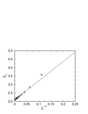
Figure 8: The SUB2 termination point as a function of $L^{-2}$ defined in Eq. (97) in 1 space dimension, using the CCM operatorial form.

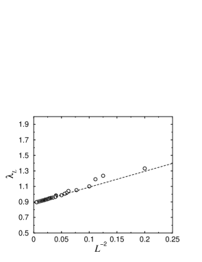
Figure 9: The SUB2 termination point as a function of $L^{-2}$ defined in Eq. (97) in 2 space dimensions, using the CCM operatorial form.

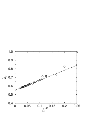
Figure 10: The SUB2 termination point as a function of $L^{-2}$ defined in Eq. (97) in 3 space dimensions, using the CCM operatorial form.

To our surprise, and somewhat to our dismay, we find that both the functional and operatorial methods predict a termination point, possibly indicative of a phase transition, in one dimension. This probably shows a defect in our approximation scheme, since no transition of this type is expected for such a one-dimensional system, and the exact results by Polyakov and Wiegmann [6] for the Euclidean theory also show no phase transition. The positions of the calculated termination points are surprisingly similar for the two approaches in all numbers of spatial dimensions, however. We also believe that both calculations have converged, so there is no obvious numerical explanation for the small differences.

Of course we have not yet addressed the important issue of whether our results indicating a phase transition at finite $\lambda$ survive in higher-order approximations. It will be interesting to pursue this matter, especially for the 1D case (where such a more sophisticated calculation to incorporate correlations between triplets or other $n$-body clusters with $n>2$ may be more feasible than in higher spatial dimensionality).

dimension	$\lambda_{\infty}$
	functional	operatorial
1	1.927	2.088
2	0.827	0.887
3	0.536	0.552

Table 1: The extrapolated CCM SUB2 termination points for the functional and operatorial methods.

6.4 Excitations

Figure 11: The excitation energy as a function of $\lambda$ in 1 space dimension in the CCM SUB2 approximations. The solid line is the RPA result from the operatorial approach; the dashed line the values obtained using the Feynman technique in the functional approach, and the dashed-dotted line the corresponding RPA result using the functional approach.

Figure 12: The excitation energy as a function of $\lambda$ in 2 space dimensions in the CCM SUB2 approximations. For the meaning of the lines see Fig. 11.

Figure 13: The excitation energy as a function of $\lambda$ in 3 space dimensions in the CCM SUB2-$n$-$m$ approximations at the highest practical truncation indices $n$ and $m$. Note that (for three dimensions) convergence in the index $n$ near the termination point is not fully attained. For the meaning of the lines see Fig. 11.

Excitation energies were evaluated by the linear response technique, for both the functional and operatorial CCM methods, as well as by Feynman’s technique for the functional method only. The solutions for 1,2, and 3 dimensions are given in Figs. 11–13. In all three cases we find that the excitation energy obtained from the Feynman technique lies above that obtained from the corresponding linear response (RPA) technique. As we approach the termination points the excitation energies approach zero rapidly. However, since the numerical calculations become unstable at the the termination point, Feynman’s technique only gives a very strong indication that at this point the system becomes gapless.

The RPA linear response methods, where we expand around the ground-state solution, give slightly lower values for the excitation energy. In these calculations the excitation can be tracked all the way to the termination point, where the system becomes gapless. There is some doubt whether the extremely small difference between the point where the solution terminates and where the RPA frequency goes through zero is due to numerical artefacts or has some physical significance, indicating that only the full SUB2 calculation will be exactly gapless at the termination point. This might, a priori, be expected since only the full SUB2 calculation contains the arbitrarily long-range correlations needed precisely at a phase transition point.

So what is the interpretation of the phase transitions that we have seen? We have investigated the eigenvectors for the mode that becomes (almost) gapless, but unfortunately the structure of these vectors, which tell us about the excitation operators to the new vacuum, do not seem to show any discernable regularity. This is probably related to the inability of the present method to describe the state beyond the putative phase transition.

Figure 14: The excitation energy as a function of $\lambda$ in 1 space dimension using the operatorial form of the CCM in SUB2 approximation, showing both the physical and unphysical branches.

The study of the linear response also allows us to display most vividly the occurrence of two branches in the energy spectrum. In Fig. 14 we show the lowest excited state, where we follow the solution of the 1D SUB2-$n$ equations to the “termination point” and beyond. At this point the solution turns around, and we find a second solution for each value of $\lambda$ where the ground-state energy is extremely close to the one from the physical solution (so close that it is impossible to distinguish the differences in the figures). We can follow this solution until we return close to the point $\lambda=0$, where some of the CCM coefficients diverge. The excitation energy in this second branch is negative, a not very desirable situation. However, the fact that the second branch does not return to the known physical ground state at $\lambda=0$, and that the excitation energies are negative leads us to denote this branch as being unphysical, an artefact of the CCM.

6.5 Comparison with other work

There exist only two sets of results with which we can easily and directly compare our results, namely the calculation by Chin [11] using the CBF technique, and a calculation using the strong-coupling expansion by Sobelman [21].

Sobelman has calculated the strong-coupling expansion in a Hamiltonian framework for a general $O(N)$ system in an arbitrary number of spatial dimensions up to fourth order. If we use his results to calculate the coupling constant for which the mass gap disappears we find systematically larger values for the (2+1)- and the (3+1)-dimensional models, by a factor of about 3, than obtained by our results. In the third-order expansion there is a vanishing mass gap for (1+1) dimensions at the critical value $\lambda=8$, but this criticality disappears in the fourth order. There remains a dip in the excitation energy around $\lambda=8$ where it crossed the zero axis before. From the exact results this seems to be the correct behaviour. However, the large change between third and fourth orders suggests that the expansion has not converged for the (1+1) model in this regime. For (2+1) and (3+1) dimensions the positions of the vanishing mass gap change somewhat, as one goes from third order to fourth order (and see Table 2). The convergence properties of the series are, however, completely unknown.

dimension	$\lambda_{\infty}$
	third order	fourth order
1	8.	–
2	2.624	2.464
3	1.637	1.492

Table 2: The coupling constants for which the excitation energies vanishes, determined from Sobelman’s strong coupling expansion.

Because of a different definition of the kinetic energy operator, the value obtained by Chin [11] for the critical coupling constant needs to be multiplied by a factor of four to agree with our definition of the model Hamiltonian given by Eq. (7). His results are for three dimensions only and he finds a critical coupling constant of $\lambda\approx 0.96$ (after scaling) compared to our results $\lambda_{\infty}=0.54$ from the SUB2 functional form and $\lambda_{\infty}=0.55$ from the SUB2 operatorial operatorial. However, more strikingly, he finds a first-order phase transition, while all our results indicate a second-order phase transition.

7 Conclusions and outlook

Our results are an interesting albeit still limited approach to a nontrivial field theory which exhibits a phase transition. They show that we can construct two different CCM-like approaches for field theories, which are amenable to different sets of approximations. For similar truncations the two methods produce very similar results.

In one space dimension we would not have expected a termination point or a phase transition from known exact results. The fact that in our approximations the termination point occurs at a large value of $\lambda$ shows that it is probably not stable against the correlations missing from our SUB2 calculations. The corresponding stability of our results in two and three spatial dimensions is certainly also of interest. The current calculations cannot address this issue, since they would have to be supplemented by complicated higher-order calculations in order to make stringent statements. This further raises the question whether one should not aim to apply the extended coupled cluster method (ECCM) [22] to the present problem. The ECCM generally has been shown to be more powerful than the normal (NCCM) version of the CCM used here in describing states on both sides of a phase transition, and might give us an idea of its nature. We believe that this might be an interesting problem for a future study.

Finally it would be appealing to look at real gauge field theories such as compact QED, or even QCD, in the light of our results. We plan to see whether the lessons we have learned in this work have any relevance for the methods of Refs. [13, 14]. We believe that armed with our arsenal of techniques we should be ready to tackle such problems, and even be able to proceed towards the inclusion of dynamical quarks in such calculations

Acknowledgement

We acknowledge support through a research grant from the Engineering and Physical Sciences Research Council (EPSRC) of Great Britain.

Appendix A Quantisation

The systematic quantisation of the non-linear sigma model is highly nontrivial. Using the components of the unit vector $\hat{n}$ as degrees of freedom, the constraint among them ($\hat{n}^{2}=1$) leads to a second constraint from the time independence of the first constraint. The Dirac brackets, which restrict the quantised operators to the physical subspace, are not particularly difficult to deal with [23], but they lead to a form that does not readily lend itself to the kind of techniques we would like to apply. One can also avoid using constraints by using an exponential parametrisation, $U=e^{i\mathbf{\tau}\cdot\mathbf{\theta}}$. However, this leads to even more complicated expressions.

We choose to use the unit vectors $\hat{n}$ as degrees of freedom, but avoid the use of constraints by using an Euler angle parametrisation of these vectors,

$$\hat{n}=(\sin\theta\sin\phi\sin\chi,\sin\theta\sin\phi\cos\chi,\sin\theta\cos\phi,\cos\theta),$$ (98)

with $0<\theta<\pi$, $0<\phi<\pi$, and $0<\chi<2\pi$. Since the Laplacian is separable in spherical coordinates, we find that the kinetic energy $K$ at a single lattice point is just the half of the angular part of the Laplacian, which is proportional to the Casimir invariant of the relevant $O(N)$ group. The kinetic energy can be derived from the generalized angular momentum operators

$$L_{ij}=-i(n_{i}\partial_{n_{j}}-n_{j}\partial_{n_{i}}),$$ (99)

where $i,j=1,2,\cdots,N$. Specifically, it may can be expressed as (the $O(N)$ Casimir invariant or) the sum-of-squares of the angular momentum operators,

$$2K=\sum^{N}_{i<j}L_{ij}^{2}=-\partial^{2}_{\theta}-(N-2)\cot\theta\partial_{\theta}-\frac{1}{\sin^{2}\theta}\partial_{\phi}^{2}-\frac{(N-3)\cot\phi}{\sin^{2}\theta}\partial_{\phi}-\frac{1}{\sin^{2}\theta\sin^{2}\phi}\partial^{2}_{\chi}+\cdots$$ (100)

In many cases we shall only need the $\theta$-dependent part, which can be rewritten in terms of $\cos\theta$ as

$$-(1-\cos^{2}\theta)\partial^{2}_{\cos\theta}+(N-1)\cos\theta\partial_{\cos\theta}.$$ (101)

Appendix B Gegenbauer polynomials

The Gegenbauer polynomials, $C^{\alpha}_{n}(x)$, are orthogonal polynomials on the domain $[-1,1]$ with respect to the weight $(1-x^{2})^{\alpha-1/2}$. The integration measure for the azimuthal angle on an $N$-dimensional sphere is $\sin^{N-2}\theta$, which means that orthogonal functions on the $N$-sphere are $C^{\alpha}_{n}(\cos\theta)$ with $\alpha=(N-2)/2$. The Gegenbauer polynomials are eigenfunctions of the kinetic energy operator

$$-[(1-x^{2})\partial_{x}^{2}-(N-1)x\partial_{x}]C^{(N-2)/2}_{n}(x)=n(n+N-2)C^{(N-2)/2}_{n}(x).$$ (102)

For $N<4$ there is a second, non-singular set of eigenfunctions of the relative angle

$$-[(1-x^{2})\partial_{x}^{2}-(N-1)x\partial_{x}](1-x^{2})^{(3-N)/2}C^{(4-N)/2}_{n}(x)=(n+1)(n-N+3)C^{(4-N)/2}_{n}(x),$$ (103)

which coincides with the first set of solutions for $N=3$, and leads to a set of sine functions for $N=2$. For a general discussion of the properties of the Gegenbauer polynomials we refer to [24]. Here we shall just summarise a few key points.

One relation that we shall use frequently in the paper is related to the addition theorem for Gegenbauer polynomials. This occurs in the integration over intermediate points in a chain of functions linking sets of lattice points. Only products of Gegenbauer polynomials of the same order contribute to the integral. This holds for arbitrary dimensions, and allows us to extend our methods to any $O(N)$ theory. Using the addition theorem for Gegenbauer polynomials

$$C_{n}^{\alpha}(\cos\theta_{1}\cos\theta_{2}+\sin\theta_{1}\sin\theta_{2}\cos\phi)=$$

$$\frac{\Gamma(2\alpha-1)}{\Gamma^{2}(\alpha)}\sum_{m=0}^{n}\frac{2^{2m}\Gamma(n-m+1)(\Gamma(\alpha+m))^{2}}{\Gamma(n+2\alpha+m)}(2\alpha+2m-1)$$

$$\times(\sin\theta_{1})^{m}(\sin\theta_{2})^{m}C_{n-m}^{\alpha+m}(\cos\theta_{1})C_{n-m}^{\alpha+m}(\cos\theta_{2})C^{\alpha-\frac{1}{2}}_{m}(\cos\phi),$$ (104)

and orthogonality of the Gegenbauer polynomials it follows that

$$\int\frac{d\mu(n_{\mathbf{i}})}{\Omega_{N}}C^{\alpha}_{k}(\hat{n}_{\mathbf{i}}\cdot\hat{n}_{\mathbf{j}})C^{\alpha}_{l}(\hat{n}_{\mathbf{i}}\cdot\hat{n}_{\mathbf{p}})=\frac{\sqrt{\pi}\Gamma(1+\alpha)4^{1-\alpha}\Gamma(2\alpha-1)}{\Gamma^{2}(\alpha)(\alpha+k)\Gamma(\alpha+1/2)}\delta_{kl}C^{\alpha}_{k}(\hat{n}_{\mathbf{j}}\cdot\hat{n}_{\mathbf{p}}).$$ (105)

When integrating over closed loops this general property implies that only “local terms” contribute, i.e., products of Gegenbauer polynomials of identical order. For $N=4$ where $\alpha=1$ this reduces to

$$\int\frac{d\mu(n_{i})}{\Omega_{4}}U_{k}(\hat{n}_{i}\cdot\hat{n}_{j})U_{l}(\hat{n}_{i}\cdot\hat{n}_{p})=\frac{\delta_{kl}U_{k}(\hat{n}_{j}\cdot\hat{n}_{p})}{1+k},$$ (106)

where $C^{1}_{n}(\cos\theta)\equiv U_{n}(\cos\theta)$ is the Chebyshev polynomial of the second kind.

The fact that the derivative of a polynomial is again a polynomial allows us to express the derivative of a Gegenbauer polynomial as a weighted sum of Gegenbauer polynomials

$$\partial_{x}C^{\alpha}_{n}(x)=\sum_{i=0}^{[n/2]}2(n-1+\alpha-2i)C^{\alpha}_{n-2i-1}(x).$$ (107)

We shall apply this transformation for the case where $n\neq 0$ (we exclude a constant part from our correlation functions). In that case we can define a matrix $T$ by

$$T_{nm}=\sum_{i=0}^{[n/2]}2(m+\alpha)\delta_{m,n-2i-1},$$ (108)

which in the subspace of interest is invertible. This linear operator $T$ is used in Eq. (96) in the RPA for the collective excited states.

References

- [1] J.F. Donoghue, E. Golowich, and B.R. Holstein, Dynamics of the Standard Model, Cambridge Press, Cambridge (1992).
- [2] M. Gell-Mann, R. Oakes, and B. Renner, Phys. Rev. 175 (1968) 2195.
- [3] G.E. Brown and M. Rho, Phys. Rev. Lett. 66 (1991) 2720.
- [4] G. Bunatian and J. Wambach, Phys. Lett. B336 (1994) 290.
- [5] M.A. Nowak, M. Rho, and I. Zahed, Chiral Nuclear Dynamics, World Scientific, Singapore (1996).
- [6] A. Polyakov and P.B. Wiegmann, Phys. Lett. B131 (1983) 121.
- [7] R.D. Pizarski and F. Wilczek, Phys. Rev. D 29 (1984) 338.
- [8] E. Brézin, J. Zinn-Justin, and J.C. Le Guillou, Phys. Rev. D 14 (1976) 2615.
- [9] P. Butera and M. Comi, Phys. Rev. B 54 (1996) 15828; M. Lüscher and P. Weisz, Nucl. Phys. B300[FS22] (1988) 325 (and references contained therein); J. Kogut. M. Snow, and M. Stone, Nucl. Phys. B200[FS4] (1982) 211.
- [10] H.E. Stanley, Phys. Rev. 176 (1968) 718.
- [11] S.A. Chin, Advances in Quantum Many-Body Theory, Vol. 1, (eds.) D. Neilson and R.F. Bishop, World Scientific, Singapore (1998), to be published.
- [12] R.F. Bishop, Theor. Chim. Acta 80 (1991) 95.
- [13] S.J. Baker, R.F. Bishop, and N.J. Davidson, Phys. Rev. D 53 (1996) 2610.
- [14] S.J. Baker, R.F. Bishop, and N.J. Davidson, Nucl. Phys. B (Proc. Supp.) 53 (1997) 834.
- [15] J. Arponen, Phys. Rev. A 55 (1997) 2686.
- [16] R.F. Bishop, J.B. Parkinson and Y. Xian, Phys. Rev. B 44 (1991) 9425.
- [17] M. Abramowitz and I. Stegun, Handbook of Mathematical Functions, National Bureau of Standards, Applied Mathematics Series 55, Washington, D.C. (1964).
- [18] W.C. Rheinboldt, Methods for Solving Systems of Nonlinear Equations, SIAM, Philadelphia, (1987); Numerical analysis of parametrized nonlinear equations, Wiley, New York (1986).
- [19] W.C. Rheinboldt and J. Burkardt, ACM TOMS 9 (1983) 236.
- [20] N.D. Mermin and H. Wagner, Phys. Lett. 17 (1966) 1133.
- [21] C.J. Hamer, J.B. Kogut, and L. Susskind, Phys. Rev. D 19 (1979) 3091; G.E. Sobelman, Phys. Rev. B 24 (1981) 1493.
- [22] J. Arponen, Ann. Phys. (N.Y.) 151 (1983) 311.
- [23] D.P. Cebula, A. Klein, and N.R. Walet, Phys. Rev. D 47 (1993) 2113.
- [24] W. Magnus, F. Oberhettinger, and R.P. Soni, Formulas and Theorems for Special Functions of Mathematical Physics, Springer-Verlag, Berlin (1966).