The Hybrid Monte Carlo Algorithm for Quantum Chromodynamics

Abstract

The Hybrid Monte Carlo (HMC) algorithm currently is the favorite scheme to simulate quantum chromodynamics including dynamical fermions. In this talk—which is intended for a non-expert audience—I want to bring together methodical and practical aspects of the HMC for full QCD simulations. I will comment on its merits and shortcomings, touch recent improvements and try to forecast its efficiency and rôle in future full QCD simulations.

1 Introduction

The Hybrid Monte Carlo algorithm [DUANE87] is—for the present—a culmination in the development of practical simulation algorithms for full quantum chromodynamics (QCD) on the lattice. QCD is the theory of the strong interaction. In principle, QCD can describe the binding of quarks by gluons, forming the hadrons with their masses, as well as other hadronic properties. As QCD cannot be evaluated satisfactorily by perturbative methods, one has to recourse to non-perturbative stochastic simulations of the quark and gluon fields on a discrete 4-dimensional space-time lattice [CREUTZ]. In analogy to simulations in statistical mechanics, in a Markov chain, a canonical ensemble of field configurations is generated by suitable Monte Carlo algorithms. As far as full QCD lattice simulations are concerned, the HMC algorithm is the method of choice as it comprises several important advantages:

• The evolution of the gluon fields through phase space is carried out simultaneously for all d.o.f., as in a molecular dynamics scheme, using the leap-frog algorithm or higher order symplectic integrators.

• Dynamical fermion loops, represented in the path-integral in form of a determinant of a huge matrix of dimension $O(10^{7})$ elements, i. e. a highly non-local object that is not directly computable, can be included by means of a stochastic representation of the fermionic determinant. This approach amounts to the solution of a huge system of linear equations of rank $O(10^{7})$ that can be solved efficiently with modern iteration algorithms, so-called Krylov-subspace methods [FROMMER94, FISCHER96].

• As a consequence, the computational complexity of HMC is a number $O(V)$, i. e., one complete sweep (update of all V d.o.f.) requires $O(V)$ operations, as it is the case for Monte Carlo simulation algorithms of local problems.

• HMC is exact, i. e. systematic errors arising from finite time steps in the molecular dynamics are eliminated by a global Monte Carlo decision.

• HMC is ergodic due to Langevin-like stochastic elements in the field update.

• HMC shows surprisingly short autocorrelation times, as recently demonstrated [SESAM97AUTO]. The autocorrelation determines the statistical significance of physical results computed from the generated ensemble of configurations.

• HMC can be fully parallelized, a property that is essential for efficient simulations on high speed parallel systems.

• HMC is computation dominated, in contrast to memory intensive alternative methods [LUESCHER94, SLAVNOV95]. Future high performance SIMD (single addressing multiple data) systems presumably are memory bounded.

In view of these properties, it is no surprise that all large scale lattice QCD simulations including dynamical Wilson fermions as of today are based on the HMC algorithm. Nevertheless, dynamical fermion simulations are still in their infancy. The computational demands of full QCD are huge and increase extremely if one approaches the chiral limit of small quark mass, i. e. the physically relevant mass regime of the light u and d quarks. The central point is the solution of the linear system of equations by iterative methods. The iterative solver, however, becomes increasingly inefficient for small quark mass. We hope that these demands can be satisfied by parallel systems of the upcoming tera-computer class [SCHILLING97].

The HMC algorithm is a general global Monte Carlo procedure that can evolve all d.o.f. of the system at the same instance in time. Therefore it is so useful for QCD where due to the inverse of the local fermion matrix in the stochastic representation of the fermionic determinant the gauge fields must be updated all at once to achieve $O(V)$ complexity. The trick is to stay close to the surface of constant Hamiltonian in phase space, in order to achieve a large acceptance rate in the global Monte Carlo step.

HMC can be applied in a variety of other fields. A promising novel idea is the merging of HMC with the multi-canonical algorithm [BERG] which is only parallelizable within global update schemes. The parallel multi-canonical procedure, can be applied at the (first-order) phase transitions of compact QED and Higgs-Yukawa model. Another example is the Fourier accelerated simulation of polymer chains as discussed in Anders Irbäck’s contribution to these proceedings, where HMC well meets the non-local features of Fourier acceleration leading to a multi-scale update process.

The outline of this talk is as follows: In section 2, a minimal set of elements and notions from QCD, necessary for the following, is introduced. In section 3, the algorithmic ingredients and computational steps of HMC are described. In section 4, I try to evaluate the computational complexity of HMC and suggest a scaling rule of the required CPU-time for vanishing Wilson quark mass. Using this rule, I try to give a prognosis as to the rôle of HMC in future full QCD simulations in relation to alternative update schemes.

2 Elements of Lattice QCD

I intend to give a pedagogical introduction into the HMC evaluation of QCD in analogy to Monte Carlo simulations of statistical systems. Therefore, I avoid to focus on details. I directly introduce the physical elements on the discrete lattice that are of importance for the HMC simulation. For the following, we do not need to discuss their parentage and relation to continuum physics in detail.

QCD is a constituent element of the standard model of elementary particle physics. Six quarks, the flavors up, down, strange, charm, bottom, and top interact via gluons. In 4-dimensional space-time, the fields associated with the quarks, $\psi^{\alpha}_{a}(\vec{x})$ have four Dirac components, $\alpha=1,\dots,4$, and three color components, $a=1,\dots,3$. The ‘color’ degree of freedom is the characteristic property reflecting the non-abelian structure of QCD as a gauge theory. This structure is based on local SU(3) gauge group transformations acting on the color index.

The gluon field $A_{\mu}^{a}(\vec{x})$ consists of four Lorentz-vector components, $\mu=1,\dots,4$. Each component carries an index $a$ running from $1$ to $8$. It refers to the components of the eight gluon field in the basis of the eight generators $\lambda_{a}$ of the group SU(3). The eight $3\times 3$ matrices $\lambda_{a}/2$ are traceless and hermitean defining the algebra of SU(3) by $[\frac{\lambda_{i}}{2},\frac{\lambda_{j}}{2}]=i\,f_{ijk}\,\frac{\lambda_{k}}{2}.$

On the lattice, the quark fields $\psi_{\vec{n}}$ are considered as approximations to the continuum fields $\psi(\vec{x})$, with $\vec{x}=a\vec{n}$, $\vec{n}\in{\bf N^{4}}$ (All lattice quantities are taken dimensionless in the following.). As shown in Fig. 1, they ‘live’ on the sites. Their fermionic nature is expressed by anti-commutators,

$$[\psi^{\alpha}_{\vec{n}},\psi^{\beta}_{\vec{m}}]_{+}=[\psi^{\dagger\alpha}_{\vec{n}},\psi^{\beta}_{\vec{m}}]_{+}=[\psi^{\dagger\alpha}_{\vec{n}},\psi^{\dagger\beta}_{\vec{m}}]_{+}=0,$$ (1)

characterizing the quark fields as Grassmann variables.

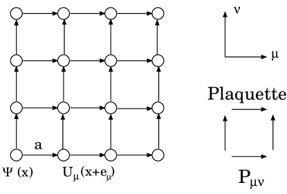
Figure 1: 2-dimensional projection of the 4-dimensional euclidean space-time lattice.

The gluon fields in the 4-dimensional discretized world are represented as bi-local objects, the so-called links $U_{\mu}(\vec{n})$. They are the bonds between site $\vec{n}$ and site $\vec{n}+{\vec{e}}_{\mu}$, with ${\vec{e}}_{\mu}$ being the unit vector in direction $\mu$. Unlike the continuum gluon field, the gluon in discrete space is $\in$ SU(3). $U_{\mu}(\vec{n})$ is a discrete approximation to the parallel transporter known from continuum QCD, $U(x,y)=\exp{(ig_{s}\int_{\vec{x}}^{\vec{y}}d{x^{\prime}}^{\mu}\,A_{\mu}^{a}(\vec{x}^{\prime})\lambda_{a}/2)}$, with $g_{s}$ being the strong coupling constant.

QCD is defined via the action $S=S_{g}+S_{f}$ that consists of the pure gluonic part and the fermionic action. The latter accounts for the quark gluon interaction and the fermion mass term. Taking the link elements from above one can construct a simple quantity, the plaquette $P_{\mu\nu}$, see Fig. 1:

$$P_{\mu\nu}(\vec{n})=U_{\mu}(\vec{n})U_{\nu}(\vec{n}+{\vec{e}}_{\mu})U^{\dagger}_{\mu}(\vec{n}+{\vec{e}}_{\nu})U^{\dagger}_{\nu}(\vec{n}).$$ (2)

The Wilson gauge action is defined by means of the plaquette:

$$\beta S_{g}=\frac{6}{{g_{s}}^{2}}\sum_{\vec{n},\mu,\nu}\left[1-\frac{1}{2}\mbox{Tr}(P_{\mu\nu}(\vec{n})+P^{\dagger}_{\mu\nu}(\vec{n}))\right].$$ (3)

In the limit of vanishing lattice spacing, one can recover the continuum version of the gauge action, $-\int d^{4}\vec{x}\frac{1}{4}F_{\mu\nu}(\vec{x})F^{\mu\nu}(\vec{x})$. The deviation from the continuum action due to the finite lattice spacing $a$ is of $O(a^{2})$.

The discrete version of the fermionic action cannot be constructed by a simple differencing scheme, as it would correspond to 16 fermions instead of 1 fermion in the continuum limit. One method to get rid of the doublers is the addition of a second order derivative term, $(\psi_{\vec{n}+{\vec{e}}_{\mu}}-2\psi_{\vec{n}}-\psi_{\vec{x}-{\vec{e}}_{\mu}})/2$, to the standard first order derivative $\gamma^{\mu}\partial_{\mu}\psi(\vec{x})\rightarrow\gamma^{\mu}(\psi_{\vec{n}+{\vec{e}}_{\mu}}-\psi_{\vec{n}-{\vec{e}}_{\mu}})/2$. This scheme is called Wilson fermion discretization. The fermionic action can be written as a bilinear form, $S_{f}=\bar{\psi}_{\vec{n}}M_{\vec{n}\vec{y}}\psi_{\vec{m}}$, with the Wilson matrix $M$,

$${M}_{\vec{n}\vec{m}}=\delta_{\vec{n}\vec{m}}-{\kappa}\sum_{\mu=1}^{4}(1-{\gamma}_{\mu}){U}_{\mu}(\vec{n})\,\delta_{\vec{n},\vec{m}-{\vec{e}}_{\mu}}(1+{\gamma}_{\mu}){U}^{\dagger}_{\mu}(\vec{n}-{\vec{e}}_{\mu})\delta_{\vec{n},\vec{m}+{{\vec{e}}_{\mu}}}.$$ (4)

The stochastic simulation of QCD starts from the analogy of the pathintegral—the quantization prescription—to a partition sum as known from statistical mechanics. As it is oscillating, it would be useless for stochastic evaluation. The appropriate framework for stochastic simulation of QCD is that of Euclidean field theory. Therefore, one performs a rotation of the time direction $t\rightarrow i\tau$. The ensuing effect is a transformation of the Minkowski metrics into a Euclidean metrics, while a positive definite Boltzmann weight $\exp(-\beta S_{g})$ is achieved. This form of the path-integral, i. e. the partition function, is well known from statistical mechanics:

$$Z=\int\left(\prod_{\vec{n},{\mu}}[d{U_{\mu}}(\vec{x})][d{\bar{\psi}_{\vec{n}}}][d\psi_{\vec{n}}]\right)e^{-\beta S_{g}-{S}_{f}}.$$ (5)

It is important for the following that one can integrate out the bilinear $S_{f}$ over the Grassmann fermion fields. As a result, we acquire the determinant of the fermionic matrix:

$$Z=\int\prod_{\vec{n},{\mu}}[d{U_{\mu}}(\vec{n})]\det(M[U])e^{-{\beta}{S}_{g}}.$$ (6)

3 Hybrid Monte Carlo

The Euclidean path-integral, Eq. (6), can in principle be evaluated by Monte Carlo techniques. We see that the fermionic fields do not appear in $Z$ after the integration. Hence, it suffices to generate a representative ensemble of fields $\{U_{i}\}$, $i=1,\dots,N$, and subsequently, to compute any observable along with the statistical error according to

$$\langle O\rangle=\frac{1}{N}\sum_{i=1}^{N}O_{i}[{U}_{i}]\quad\mbox{and}\quad\sigma^{2}_{O}=\frac{2\tau_{\mbox{\footnotesize int}}}{N}\left(\frac{1}{N}\sum_{i=1}^{N}|O_{i}[{U}_{i}]|^{2}-\langle O\rangle^{2}\right).$$ (7)

The integrated autocorrelation time $\tau_{\mbox{\footnotesize int}}$ reflects the fact that the members of the ensemble are generated by importance sampling in a Markov chain. Therefore, a given configuration is correlated with its predecessors, and the actual statistical error of a result is increased compared to the naive standard deviation. The length of the autocorrelation time is a crucial quantity for the efficiency of a simulation algorithm.

3.1 $O(V)$ Algorithms for full QCD

If we want to generate a series of field configurations $U_{1}$, $U_{2}$, $U_{3}$…in a Markov process, besides the requirement for ergodicity, it is sufficient to fulfill the condition of detailed balance to yield configurations according to a canonical probability distribution:

$$e^{-S}P(U\rightarrow U^{\prime})=e^{-S^{\prime}}P(U^{\prime}\rightarrow U).$$ (8)

$P(U\rightarrow U^{\prime})$ is the probability to arrive at configuration $U^{\prime}$ starting out from $U$. Let us for the moment forget about $\det(M[U])$, i. e., we set $\det(M)$ equal to 1 in Eq. (6). In that case, the action is purely gluonic (pure gauge theory), and local. Therefore, using the rules of Metropolis et al. we can update each link independently one by one by some (reversible!) stochastic modification $U_{\mu}(\vec{n})\rightarrow{U^{\prime}}_{\mu}(\vec{n})$, while only local changes in the action are induced. One ‘sweep’ is performed if all links are updated once. By application of the Metropolis rule, $P(U\rightarrow U^{\prime})=\min\left[1,\exp({-\Delta S_{g}})\right]$, detailed balance is fulfilled, and we are guaranteed to reach the canonical distribution. Starting from a random configuration, after some thermalization steps, we can assume hat the generated configurations belong to an equilibrium distribution. Without dynamical fermions—i. e. in the quenched approximation—standard Metropolis shows a complexity $O(V)$, with $V$ being the number of d.o.f.

However, if we try to use Metropolis for full QCD, the decision $P(U\rightarrow U^{\prime})=\min\left[1,\exp({-\Delta S_{g}})\frac{\det(M[U^{\prime}])}{\det(M[U])}\right]$ would imply the evaluation of the fermionic determinant for each ${U}_{\mu}(\vec{n})$ separately. A direct computation of the determinant requires $O(V^{3})$ operations and therefore, the total computational complexity would be a number $O(V^{4})$.

These implications for the simulation of full QCD with dynamical fermions have been recognized very early. In a series of successful steps, the computational complexity could be brought into the range of quenched simulations. The following table gives an (incomplete) picture of this struggle towards exact, ergodic, practicable and parallelizable $O(V)$ algorithms for full QCD.

Table 1: Towards exact and ergodic $O(V)$ algorithms.

Method	order	exact	ergodic	year
Metropolis	$V^{4}$	yes	yes	Metropolis et al. 1953
Pseudo Fermions	$V^{2}$	no	yes	Fucito et al. 1981
Gauss Representation	$V^{2}$	yes	yes	Petcher, Weingarten 1981
Langevin	$V$	no	yes	Parisi, Wu 1981
Microcanonical	$V$	no	no	Polonyi at al. 1982
Hybrid Molecular Dynamics	$V$	no	yes	Duane 1985
HMC	$V$	yes	yes	Duane et al. 1987
Local Bosonic Algorithm	$V$	no	yes	Lüscher 1994
Exact LBA	$V$	yes	yes	DeForcrand et al. 1995
5-D Bosonic Algorithm	$V$	no	yes	Slavnov 1996

A key step was the introduction of the fermionic determinant by a Gaussian integral. As a synthesis of several ingredients, HMC is a mix of Langevin simulation, micro-canonical molecular dynamics, stochastic Gauss representation of the fermionic determinant, and Metropolis.

3.2 Hybrid Monte Carlo: Quenched Case

For simplicity, I first discuss the quenched approximation, i. e. $\det(M)=\mbox{const.}$ Each sweep of the HMC is composed of two steps:

1. The gauge field is evolved through phase space by means of (micro-canonical) molecular dynamics. To this end, an artificial guidance Hamiltonian $\cal H$ is introduced adding the quadratic action of momenta to $S_{g}$, “conjugate” to the gauge links. The micro-canonical evolution proceeds in the artificial time direction as induced by the Hamiltonian. Choosing random momenta at the begin of the trajectory, ergodicity is guaranteed, as it is by the stochastic force in the Langevin algorithm. In contrast to Langevin, HMC carries out many integration steps between the refreshment of the momenta.

2. The equations of motion are chosen to conserve ${\cal H}$. In practice, a numerical integration can conserve $\cal H$ only approximately. However, the change $\Delta{\cal H}={\cal H}_{f}-{\cal H}_{i}$ is small enough to lead to high acceptances of the Metropolis decision—rendering HMC exact, the essential improvement of HMC compared to the preceding hybrid-molecular dynamics algorihm.

With

$${\cal H}=S_{g}[U]+\frac{1}{2}\sum_{\vec{n},\mu,color}\mbox{Tr}\,H_{\mu}^{2}(\vec{n})\quad\mbox{and}\quad Z=\int[dH][dU]e^{-{\cal{H}}},$$ (9)

expectation values of observables are not altered with respect to Eq. (6), if the momenta are chosen from a Gaussian distribution. A suitable $H$ is found using the fact that $U\in$ SU(3) under the evolution. Taylor expansion of $U(\tau+\Delta\tau)$ leads to $U(\tau)\dot{U}^{\dagger}(\tau)+\dot{U}(\tau)U^{\dagger}(\tau)=0$. This differential equation is fulfilled choosing the first equation of motion as

$$\dot{U}=iHU,$$ (10)

with $H$ represented by the generators of SU(3) and thus being hermitean and traceless, $H_{\mu}(\vec{n})=\sum_{a=1}^{8}\lambda_{a}{h_{\mu}^{a}(\vec{n})}$. Each component $h_{\mu}^{a}$ is a Gaussian distributed random number. As $\cal H$ should be a constant of motion, $\dot{\cal H}=0$, we get

$$\dot{\cal H} = \sum_{\vec{n},\mu}\mbox{Tr}\left\{H_{\mu}(\vec{n})\dot{H}_{\mu}(\vec{n})-\frac{\beta}{6}[\dot{U}_{\mu}(\vec{n})V_{\mu}(\vec{n})+h.c.]\right\}=0$$

$$\dot{\cal H} = \sum_{\vec{n},\mu}\mbox{Tr}\left\{H_{\mu}(\vec{n})\left[\dot{H}_{\mu}(\vec{n})-i\frac{\beta}{6}(U_{\mu}(\vec{n})V_{\mu}(\vec{n})-h.c.)\right]\right\}=0.$$ (11)

We note that $[]\propto 1$ since $\{\}$ must be traceless. Since $\dot{H}$ must stay explicitly traceless under the evolution it follows that $[]=0$. The second equation of motion reads:

$$i\dot{H}(\vec{n})=-\frac{\beta}{6}\left\{U_{\mu}(\vec{n})V_{\mu}(\vec{n})-h.c.\right\}.$$ (12)

The quantities $V_{\mu}(\vec{n})$ corresponding to a gluonic force term are the staples, i. e. the incomplete plaquettes that arise in the differentiation,

$$V_{\mu}(\vec{n})=\sum_{\nu\neq\mu}\left\{\begin{minipage}{71.13188pt} \epsfbox{staples.eps} \end{minipage}\right\}.$$ (13)

For exact integration, the Hamiltonian $\cal H$ would be conserved. However, numerical integration only can stay close to ${\cal H}=const.$ Therefore, one adds a global Metropolis step,

$$P_{\mbox{\footnotesize acc}}=\min(1,e^{-\Delta\cal H}),$$ (14)

to reach a canonical distribution for $\{U\}$. As a necessary condition for detailed balance the integration scheme must lead to a time reversible trajectory and fulfill Liouville’s theorem, i. e. preserve the phase-space volume. Symplectic integration is the method of choice. It is stable as far as energy drifts are concerned.

3.3 Including Dynamical (Wilson) Fermions

Dynamical fermions are included in form of a stochastic Gaussian representation of the fermionic determinant in Eq. (6). In order to ensure convergence of the Gauss integral, the interaction matrix must be hermitean. Since the Wilson fermion matrix $M$ is a complex matrix, it cannot be represented directly. A popular remedy is to consider the two light quarks u and d as mass degenerate. With the identity $\det^{2}(M)=\det(M^{\dagger}M)$ the representation reads

$$\det(M^{\dagger}M)=\int\left(\prod_{\vec{n}}[d{\bar{\phi}_{\vec{n}}}][d\phi_{\vec{n}}]\right)e^{-{\phi_{\vec{n}}^{*}(M^{\dagger}M)_{\vec{n},\vec{m}}^{-1}\phi_{\vec{m}}}}.$$ (15)

The bosonic field $\phi$ can be related to a vector $R$ of Gaussian random numbers. In a heat-bath scheme, it is generated using the standard Muller-Box procedure, and with $\phi=M^{\dagger}R$, we arrive at $R^{\dagger}R$, the desired starting distribution, equivalent to $\phi^{*}(M^{\dagger}M)^{-1}\phi=\phi^{*}\,X$. Adding the fermionic action to $\cal H$, its time derivative reads:

$$\frac{dS_{f}}{d\tau} = \kappa\sum_{\vec{n},\mu}\mbox{Tr}[\dot{U}_{\mu}(\vec{n})F_{\mu}(\vec{n})+h.c.],$$

$$F_{\mu}(\vec{n}) = [MX]_{\vec{n}+{\vec{e}}_{\mu}}X^{\dagger}_{\vec{n}}(1+\gamma_{\mu})+X_{\vec{n}+{\vec{e}}_{\mu}}[MX]^{\dagger}_{\vec{n}}(1-\gamma_{\mu}).$$ (16)

$F$ is the fermionic force that modifies the second equation of motion to

$$i\dot{H}(\vec{n})=-\frac{\beta}{6}\left\{U_{\mu}(\vec{n})V_{\mu}(\vec{n})+\kappa\mbox{Tr}\,F_{\mu}(\vec{n})-h.c.\right\}.$$ (17)

3.4 Numerical Integration and Improvements

The finite time-step integration of the equation of motion must be reversible and has to conserve the phase-space volume, while it should deviate little from the surface ${\cal H}=const.$ The leap-frog scheme can fulfill these requirements. It consists of a sequence of triades of the following form:

$$H_{\mu}(\vec{n},\tau+\frac{\Delta\tau}{2}) = H_{\mu}(\vec{n},\tau)+\frac{\Delta\tau}{2}\dot{H}_{\mu}(\vec{n},\tau)$$

$$U_{\mu}(\vec{n},\tau+\Delta\tau) = e^{i\Delta\tau H_{\mu}(\vec{n},\tau+\frac{\Delta\tau}{2})}U_{\mu}(\vec{n},\tau)$$

$$H_{\mu}(\vec{n},\tau+\Delta\tau) = H_{\mu}(\vec{n},\tau+\frac{\Delta\tau}{2})+\frac{\Delta\tau}{2}\dot{H}_{\mu}(\vec{n},\tau+\Delta\tau).$$ (18)

It can be shown that the leap frog scheme approximates $\cal H$ correctly up to $O(\Delta t^{2})$ for each triade. As a rule of thumb, the time step and the number of integration steps, $N_{md}$, should be chosen such that the length of a trajectory in fictitious time is $N_{md}\times\Delta\tau\simeq O(1)$ at an acceptance rate $>70\%$. It is easy to see from the discrete equations of motion (EOM) that the phase space volume $[dH][dU]$ is conserved: loosely speaking, $dU$ is conserved as the first EOM amounts to a rotation in group space, and from the second EOM follows that $dH^{\prime}=dH$. In order to improve the accuracy of the numerical integration, one can employ higher order symplectic integrators. As the integration part of HMC is not specific for QCD, higher order integrators could be very useful for other applications as the Fourier accelerated HMC introduced by A. Irbäck.

Despite of the reduction of the computational complexity to $O(V)$, the repeated determination of the large “vector” $X$, $X=(M^{\dagger}M)^{-1}\phi$, renders the simulation of QCD with dynamical fermions still computationally extremely intensive. The size of the vector $X$ is about 1 - 20 $\times 10^{6}$ words. The code stays more than 95 % of execution time in this phase. Since typical simulations run several months in dedicated mode on fast parallel machines, any percent of improvement is welcome. Traditionally, the system was solved by use of Krylov subspace methods such as conjugate gradient, minimal residuum or Gauss-Seidel. In the last three years, improvements could be achieved by introduction of the BiCGstab solver [FROMMER94] and by use of novel parallel preconditioning techniques [FISCHER96] called local-lexicographic SSOR (symmetric successive over-relaxation). Further improvements have been achieved through refined educated guessing, where the solution $X$ of previous steps in molecular dynamics time is fed in to accelerate the current iteration [BROWER]. Altogether, a factor of about 4 up to 8 could be gained by algorithmic research.

4 Efficiency and Scaling

Apart from purely algorithmic issues, the efficiency of a Monte Carlo simulation is largely determined by the autocorrelation of the Markov chain. A significant determination of autocorrelation times of HMC in realistic full QCD with Wilson fermions could not be carried out until recently [SESAM97AUTO]. The length of the trajectory samples in these simulations was around 5000 (Here, with ‘trajectory’ we denote a new field configuration at the end of a Monte Carlo decision.). The lattice sizes were $16^{3}\times 32$ and $24^{3}\times 40.$

The finite time-series approximation to the true autocorrelation function for an observable ${\cal O}_{t}$, $t=1,\dots,t_{MC}$, is defined as

$$C^{\cal O}(t)=\frac{\sum\limits_{s=1}^{t_{MC}-t}{\cal O}_{s}{\cal O}_{s+t}-\frac{1}{t_{MC}-t}\left(\sum\limits_{s=1}^{t_{MC}}{\cal O}_{s}\right)^{2}}{t_{MC}-t}.$$ (19)

The definition of corelation in an artificial time is made in analogy to connected correlation functions in real time. The integrated autocorrelation time is defined as $\tau^{\cal O}_{int}=\frac{1}{2}+\sum_{t^{\prime}=1}^{t_{MC}\to\infty}\frac{C^{\cal O}(t^{\prime})}{C^{\cal O}(0)}.$ In equilibrium, $\tau^{\cal O}_{int}$ characterizes the statistical error of the observable ${\cal O}$.

The integrated autocorrelation times have been determined from several observables, such as the plaquette and the smallest eigenvalue of $M$. They are smaller than anticipated previously, and their length is between 10 and 40 trajectories. Therefore, one can consider configurations as decorrelated that are separated by $\tau^{\cal O}_{int}$ trajectories.

The quality of the data allowed to address the issue of critical slowing down for HMC, approaching the chiral limit of vanishing u and d quark mass, where the pion correlation length $\xi_{\pi}=1/m_{\pi}a$ is growing. The autocorrelation time is expected to scale with a power of $\xi_{\pi}$, $\tau=\epsilon\xi_{\pi}^{z}$, $z$ is called dynamical critical exponent. As a result the dynamical critical exponent of HMC is located between $z=1.3$ and 1.8 for local and extended observables, respectively.

Finally let me try to give a conservative guess of the computational effort required with HMC for de-correlation. The pion correlation length $\xi_{\pi}$ must be limited to $V^{\frac{1}{4}}/\xi_{\pi}\approx 4$ to avoid finite size effects as the pion begins to feel the periodic boundary of the lattice. With $\xi_{\pi}$ fixed, the volume factor goes as $\xi_{\pi}^{4}$. Furthermore the compute effort for BiCGstab increases $\propto\xi^{-2.7}$ [SESAM97AUTO]. In order to keep the acceptance rate constant, the time step has been reduced (from 0.01 to 0.004) with increasing lattice size ($16^{3}\times 32$ to $24^{3}\times 40$), while the number of time steps was increased from 100 to 125. Surprisingly, the autocorrelation time of the ‘worst case’ observable, the minimal eigenvalue of $M$, goes down by 30 % compensating the increase in acceptance rate cost! In a conservative estimate, the total time scales as $m_{\pi}^{-8}$ to $m_{\pi}^{-8.5}$. As a result, for Wilson fermions, the magic limit of $\frac{m_{\pi}}{m_{\rho}}<0.5$, will be in reach on $32^{3}\times L_{t}$ lattices—on a Teracomputer.

Alternative schemes like the local bosonic algorithm or the 5-dimensional bosonic scheme are by far more memory consuming than HMC. Here, a promising new idea might be the Polynomial HMC [JANSEN]. The autocorrelation times of these alternative schemes in realistic simulations are not yet known accurately, however. In view of the advantages of HMC mentioned in the introduction, and the improvements achieved, together with the our new findings as to its critical dynamics, I reckon HMC to be the method of choice for future full QCD simulations on Teralcomputers. Acknowledgments. I thank the members of the SESAM and the T$\chi$L collaborations and A. Frommer for many useful discussions.

References

- [1] DUANE87(Duane et al. 1987) Duane, S., Kennedy, A., Pendleton, B., Roweth, D. (1987): Phys. Lett. B195, 216
- [2] CREUTZ(Creutz 1983) Creutz, M. (1983): Lattice Gauge Theory (Cambridge University Press, Cambridge)
- [3] FROMMER94(Frommer et al. 1994) Frommer, A. et al. (1994): Int. J. Mod. Phys. C5, 1073
- [4] FISCHER96(Fischer et al. 1996) Fischer, S. et al. (1996): Comp. Phys. Comm. 98, 20-34
- [5] SESAM97AUTO(SESAM collaboration 1997) Sesam collaboration, to appear
- [6] BROWER(Brower et al. 1997) R. C. Brower, et. al. (1997): Nucl. Phys. B484, 353-374
- [7] LUESCHER94(Luescher 1994) Luescher, M. (1994): Nucl. Phys. B418, 637-648
- [8] SLAVNOV95(Slavnov 1996) Slavnov, A. (1996): Preprint SMI-20-96, 6pp
- [9] SCHILLING97(Schilling 1997) Schilling, K. (1997): TERAcomputing in Europa: Quo Vamus? Phys. Bl. 10, 976-978
- [10] BERG(Berg & Neuhaus 1992) Berg, B. A. and Neuhaus, T. (1992): Phys. Rev. Lett. 68, 9-12
- [11] CHENGLICheng & Li, 1989 Cheng, T.-P. Li, L.-F. (1989): Gauge Theory of Elementary Particle Physics (Claredon Press, Oxford)
- [12] JANSEN(Frezzotti & Jansen) Frezzotti, R., Jansen, K. (1997) Phys. Lett. B402, 328-334