CERN-TH/97-332

hep-lat/9711048

November 1997

Three-dimensional U(1) gauge+Higgs theory as an effective
theory for finite temperature phase transitions

K. Kajantie^a,b, M. Karjalainen^b, M. Laine^a, J. Peisa^c

^aTheory Division, CERN, CH-1211 Geneva 23, Switzerland
^bDepartment of Physics, P.O.Box 9, 00014 University of Helsinki, Finland
^cDepartment of Mathematical Sciences, University of Liverpool,
Liverpool L69 3BX, UK

Abstract

We study the three-dimensional U(1)+Higgs theory (Ginzburg-Landau model) as an effective theory for finite temperature phase transitions from the 1 K scale of superconductivity to the relativistic scales of scalar electrodynamics. The relations between the parameters of the physical theory and the parameters of the 3d effective theory are given. The 3d theory as such is studied with lattice Monte Carlo techniques. The phase diagram, the characteristics of the transition in the first order regime, and scalar and vector correlation lengths are determined. We find that even rather deep in the first order regime, the transition is weaker than indicated by 2-loop perturbation theory. Topological effects caused by the compact formulation are studied, and it is demonstrated that they vanish in the continuum limit. In particular, the photon mass (inverse correlation length) is observed to be zero within statistical errors in the symmetric phase, thus constituting an effective order parameter.

1 Introduction

Finite temperature phenomena are very important for cosmology and for the physics of ultrarelativistic heavy ion collisions. It is thus indispensable to have efficient and accurate methods for computing, e.g., the partition function for a given theory. This paper is devoted to solving this problem for the U(1) gauge+Higgs theory, or scalar electrodynamics, or the Ginzburg-Landau model. This theory in three dimensions is the effective theory of superconductivity [1] and of liquid crystals [2] in certain regimes, and it is also an interesting theoretical laboratory for studying the thermodynamics of and topological defect formation in relativistic field theories.

A finite temperature system singles out a specific Lorentz frame, the rest frame of the matter. In non-relativistic condensed matter physics this automatically leads to a three-dimensional (3d) — or in some cases even lower dimensional — formulation of thermodynamical computations. The Hamiltonian is given and the partition function is computed in 3d. For realistic systems the full computation is usually too complicated and one has to replace the original theory by an effective one focussing on the essential degrees of freedom. For instance, in superconductivity the full quantum theory of electrons in an ionic lattice is first replaced by the BCS theory, which then for a class of phenomena can be replaced by the very simple Ginzburg-Landau model [1].

The situation is different in finite temperature relativistic field theories. The general first-principles Lorentz and gauge invariant formulation is necessarily four-dimensional (4d). However, even here, for a class of theories and phenomena, the full 4d theory can be replaced by effective 3d theories of various degrees of simplicity. The original idea [3–5] is rather old and has recently been applied to a large class of relativistic field theories, such as QCD [6–9], the SU(2)+fundamental Higgs theory or the Standard Model [10–13], the Minimal Supersymmetric Standard Model [14–17], and the SU(5)+adjoint 24-plet Higgs theory [18]. The corresponding 3d effective theories have been numerically studied for QCD in [19–21,9], for SU(2)+fundamental Higgs in [10,22–27], and for SU(2)$\times$U(1) + fundamental Higgs in [28]. The present case of the U(1)+Higgs theory, for which dimensional reduction has been considered in [12,29–31] has been numerically studied in [32–38].

The purpose of this paper is to study the U(1)+Higgs theory in the effective theory approach, emphasizing the two essential but totally separate aspects of the problem:

• The numerical study of the 3d effective theory as such: the determination of the phase diagram, of the characteristics of the phase transitions found, and of the correlation lengths of various gauge invariant operators. We have presented our first results for the correlation length measurements and for the structure of the phase diagram already in [38], and here we concentrate on the characteristics of the phase transition in the 1st order regime and on explaining the details of the correlation length measurements. Earlier numerical work has appeared in [32–37]. The full solution of the problem requires this numerical work, although analytic methods [39–44] give important insights, as well. It is also quite interesting to compare the U(1)+Higgs theory with several related theories with a massless photon in the tree-level spectrum: SU(2)$\times$U(1) + fundamental Higgs theory [28], SU(2)+adjoint Higgs theory [21, 9] and the pure U(1) theory [45–47]. The topological mass created for the photons in the compact formulation [48–51] will play an important role in this context.

• The analytic derivation of the relation between the full physical theory and the effective theory. Here many different physical theories can be mapped onto one effective theory. The U(1)+Higgs theory is particularly interesting in that the full theory can be, e.g., superconductivity at $T\sim$ 1 Kelvin or hot scalar+fermion plasma at relativistic temperatures. Of course, the latter case can also be approached directly from the 4d viewpoint [52, 53].

The results for the first aspect — the numerical study of the 3d theory as such — are contained in Sections 2–6 of this paper. We formulate the problem in continuum in Sec. 2, make some perturbative computations in Sec. 3, discretize the theory in Sec. 4, discuss the photon in the discretized theory and in some other 3d theories in Sec. 5, and present our main lattice results in Sec. 6. Since the second aspect of the problem, the derivation of the 3d theory, completely factorizes from the first aspect, we discuss the derivation separately in Appendix A for the case of superconductivity and in Appendix B for the hot scalar+fermion plasma. We conclude in Sec. 7.

2 3d U(1)+Higgs theory in continuum

The 3d U(1)+Higgs theory is a locally gauge invariant continuum field theory defined by the functional integral

$$Z = \int{\cal D}A_{i}{\cal D}\phi\,\exp\bigl{[}-S(A_{i},\phi)\bigr{]},$$ (2.1)

$$S = \int d^{3}x\biggl{[}{\frac{1}{4}}F_{ij}^{2}+|D_{i}\phi|^{2}+m_{3}^{2}\phi^{*}\phi+\lambda_{3}\left(\phi^{*}\phi\right)^{2}\bigg{]},$$ (2.2)

where $F_{ij}=\partial_{i}A_{j}-\partial_{j}A_{i}$ and $D_{i}=\partial_{i}+ie_{3}A_{i}$. The parameters $m_{3},e_{3}^{2},\lambda_{3}$ of the Lagrangian have the dimension GeV and the fields have dimension GeV^1/2. Since the theory in eq. (2.2) is a continuum field theory, one has to carry out ultraviolet renormalization. In 3d the couplings $e_{3}^{2}$ and $\lambda_{3}$ are not renormalised in the ultraviolet, but there is a linear 1-loop and a logarithmic 2-loop divergence for the mass parameter $m_{3}^{2}$. In the $\overline{\mbox{\rm MS}}$ dimensional regularization scheme in $3-2\epsilon$ dimensions, the renormalized mass parameter becomes [12]

$$m_{3}^{2}(\mu)={-4e_{3}^{4}+8\lambda_{3}e_{3}^{2}-8\lambda_{3}^{2}\over 16\pi^{2}}\log\frac{\Lambda_{m}}{\mu},$$ (2.3)

where $\Lambda_{m}$ is a scale independent physical mass parameter of the theory. Instead of it, it is more convenient to use $m_{3}^{2}(e_{3}^{2})$. Choosing $e_{3}^{2}$ to set the scale, the physics of the theory will depend on the two dimensionless ratios

$$y={m_{3}^{2}(e_{3}^{2})\over e_{3}^{4}},\quad x={\lambda_{3}\over e_{3}^{2}}.$$ (2.4)

We shall later in Appendices A and B relate the parameters of superconductivity and finite $T$ scalar electrodynamics to $x$ and $y$.

Figure 1: The phase diagram of the G-L theory. The photon mass acts as an effective order parameter.

It is now a mathematical and computational problem to determine the physics associated with the theory in eq. (2.1). As usual all physics lies in expectation values of various operators. Since this is a gauge theory, only gauge invariant operators have non-vanishing expectation values. The most relevant of these are the local (depending only on one point x) operators of lowest dimensionalities (half-odd dimensions could be made integer by multiplying by $e_{3}$):

• Dim = 1: the $J^{PC}=0^{++}$ scalar $S(\mbox{\bf x})=\phi^{*}(\mbox{\bf x})\phi(\mbox{\bf x})$.

• Dim = 1${\frac{1}{2}}$: the $1^{+-}$ vector $\tilde{V}_{i}(\mbox{\bf x})\equiv B_{i}={\frac{1}{2}}\epsilon_{ijk}F_{jk}(\mbox{\bf x})$.

• Dim = 2: the $1^{--}$ vector $V_{i}(\mbox{\bf x})={\rm Im}\,\phi^{*}(\mbox{\bf x})D_{i}\phi(\mbox{\bf x})$; the $1^{-+}$ vector $S_{i}(\mbox{\bf x})={\rm Re}\,\phi^{*}(\mbox{\bf x})D_{i}\phi(\mbox{\bf x})=\partial_{i}\phi^{*}(\mbox{\bf x})\phi(\mbox{\bf x})$; and the $0^{++}$ scalar $(\phi^{*}\phi)^{2}$.

• Dim = 2${\frac{1}{2}}$: the $1^{+-}$ vector $\phi^{*}B_{i}\phi$.

• Dim = 3: The $0^{++}$ scalars $F_{ij}F_{ij}$ and $\phi^{*}D_{i}D_{i}\phi$; and the $2^{++}$ tensor $\phi^{*}[\{D_{i},D_{j}\}-2/d\,\,\delta_{ij}D_{k}D_{k}]\phi$; etc.

• Dim = 3${\frac{1}{2}}$: The $0^{--}$ scalar $B_{i}\,\partial_{i}\phi^{*}\phi$; and the $0^{-+}$ scalar $B_{i}\,{\rm Im}\,\phi^{*}D_{i}\phi$; etc.

• Dim = 4: The $0^{+-}$ scalar $\partial_{i}\phi^{*}\phi\,{\rm Im}\,\phi^{*}D_{i}\phi$; etc.

The quantum numbers here refer to O(3). From these one can further construct, e.g., bilocal operators such as correlators of two of the above operators acting at different points.

The first topic of importance is the phase structure of the theory. The critical curve $y=y_{c}(x)$ (see Fig. 1) divides the plane into two disjoint regions, the symmetric phase at $y>y_{c}(x)$ and the broken phase at $y<y_{c}(x)$. The presence of a critical curve is signalled by singularities in the free energy

$$Z=\exp\bigl{[}-Ve_{3}^{6}f(y,x)\bigr{]},$$ (2.5)

where $f$ is dimensionless. The critical curve is localised by measuring different local or bilocal expectation values of the gauge invariant local operators listed above. There is no local gauge invariant order parameter, the expectation value of which would vanish in one of the phases. Instead, we shall use as an effective order parameter the photon mass, which is measured from a bilocal operator.

For small $x$, the system has a first-order transition (Fig. 1). It then has two bulk states of the same free energy, and the broken and symmetric phases coexist at $y_{c}$. The system has one stable and one metastable branch for $y_{-}(x)<y<y_{+}(x)$. Expectation values of various gauge invariant scalar operators jump when crossing $y_{c}(x)$. The following quantities are of particular interest:

• The jump $\Delta\ell_{3}$ of the order parameter like quantity $\ell_{3}\equiv\langle\phi^{\dagger}\phi(e_{3}^{2})\rangle/e_{3}^{2}$ between the broken and symmetric phases at $y_{c}$. In perturbation theory, $\Delta\ell_{3}\sim{\scriptstyle{1\over 2}}\phi^{2}_{b}(y_{c})/e_{3}^{2}$, where $\phi_{b}$ is the location of the broken minimum in, say, the Landau gauge. Note that $\langle\phi^{\dagger}\phi(\mu)\rangle$ is scale dependent [54], as given below in eq. (4.6).

• The interface tension $\sigma_{3}\equiv\sigma/(Te_{3}^{4})$, defined in perturbation theory by

  $$\sigma_{3}=\int_{0}^{\phi_{b}/e_{3}}\,d(\phi/e_{3})\sqrt{2V(\phi/e_{3})/e_{3}^{6}},$$ (2.6)

  where $V$ is the perturbatively computed 3d effective potential. On the lattice $\sigma_{3}$ is determined from the fundamental relation $F=-pV+\sigma A$, which holds in the presence of a planar interface separating two coexisting phases.

In a second order transition, on the other hand, the quantities of interest are the different critical exponents.

The second essential property of the U(1)+Higgs theory is its excitation spectrum. In perturbation theory, one can easily see what the free field degrees of freedom are both in the symmetric and broken phases (see also Table 1). However, the symmetric phase is in some respects non-perturbative (since the Coulomb potential is logarithmically confining in 2+1 dimensions) and thus these states need not be the physical ones. The physical states are described by the correlators of the gauge invariant operators listed above. For example, the physical mass, or inverse correlation length, of the lowest scalar 0⁺⁺ excitation is obtained from the large distance behaviour of the correlator $\langle S(\mbox{\bf x})S({\bf y})\rangle$. To study vector 1^– excitations we shall use the operators $\tilde{V}_{i}(\mbox{\bf x}),V_{i}(\mbox{\bf x})$. In condensed matter context these masses are usually called “renormalised” masses; we prefer to reserve the word renormalisation for the elimination of ultraviolet divergences.

A particularly interesting state is the photon. It is evidently one of the fundamental fields of the action in the symmetric phase; is it in the physical spectrum of the theory? In [38] we have provided non-perturbative evidence for the fact that it indeed is. It can thus serve as an effective order parameter and the phase diagram can contain two disconnected regions as in Fig. 1. This is a nontrivial fact, since massless states can disappear from the physical spectrum or in the lattice formulation of the theory. This will be discussed in more detail in Section 5.

3 Perturbative results for the U(1)+Higgs theory

Let us consider the region of small $x$. Then perturbation theory is expected to be accurate and it predicts a “fluctuation induced” or “Coleman-Weinberg-type” first order phase transition. Renormalised perturbation theory induces a dependence on a scale $\mu$ and in 3d one has to go to 2 loops in order to optimize this scale. The 2-loop potential has been discussed in [53, 12, 30, 37] and optimisation in [12, 37], and we refer there for details (see also eq. (B.33) below for the 2-loop potential in the full 4d theory with fermions).

To show the main qualitative features of the perturbative results, consider the 1-loop potential in the Landau gauge (see eq. (B.31)),

$$V_{\mbox{\scriptsize 1-loop}}/e_{3}^{6}=\biggl{\{}{\frac{1}{2}}y(\mu){\hat{\phi}}^{2}+{\frac{1}{4}}x{\hat{\phi}}^{4}-{1\over 12\pi}\Bigl{[}2{\hat{\phi}}^{3}+(y+3x{\hat{\phi}}^{2})^{3/2}+(y+x{\hat{\phi}}^{2})^{3/2}-2y^{3/2}\Bigr{]}\biggr{\}},$$ (3.1)

where ${\hat{\phi}}=\phi/e_{3}$ and

$$y(\mu)=y+{1\over 16\pi^{2}}(-4+8x-8x^{2})\ln{e_{3}^{2}\over\mu}.$$ (3.2)

The $\mu$ dependence of $y(\mu)$ is of 2-loop order so that it is a higher order effect in eq. (3.1). The leading $x\to 0$ result is obtained by including only the 1-loop vector term, the first 1-loop term in eq. (3.1). The potential is then, equivalently,

$$V_{\rm 1-loop}/e_{3}^{6}\approx{\frac{1}{4}}x{\hat{\phi}}^{2}\biggl{[}\biggl{(}{\hat{\phi}}-{1\over 3\pi x}\biggr{)}^{2}+{2y\over x}\biggl{(}1-{1\over 18\pi^{2}xy}\biggr{)}\biggr{]}.$$ (3.3)

Two degenerate states are obtained when the last term vanishes. From this one finds that

$$y_{c}(x) = {1\over 18\pi^{2}x},\quad y_{+}(x)={1\over 16\pi^{2}x},\quad y_{-}(x)=0,$$ (3.4)

$${\hat{\phi}}_{\mbox{\scriptsize symm}} = 0,\quad{\hat{\phi}}_{\mbox{\scriptsize broken}}={1\over 3\pi x},$$ (3.5)

$$\Delta\ell_{3} = {1\over 18\pi^{2}x^{2}},\quad\sigma_{3}={2^{3/2}\over 648\pi^{3}x^{5/2}}.$$ (3.6)

Taking into account the other terms in eq. (3.1) and the 2-loop effects, one can improve on the accuracy. Perturbative results for the critical curve, the latent heat and the interface tension in different approximations are shown in Figs. 2 and 3. The curves are scaled with the leading $x\to 0$ dependences (eqs. (3.4), (3.6)). The variation as a function of $x$ in the 1-loop results is due to the scalar loop terms in eq. (3.1). The 2-loop results have been computed by either optimising [12, 37] the scale $\mu$ or by fixing it to be $\mu=e_{3}^{2}$. The scale dependence gives an idea of the magnitude of higher order corrections. One observes that perturbation theory is becoming unreliable at least for $x\mathop{\raise 1.29167pt\hbox{$>$\kern-7.5pt\raise-4.73611pt\hbox{$\sim$}}}0.1\ldots 0.2$.

Concerning the mass spectrum, using the approximations $m_{W}=e_{3}\phi_{b}$, $m_{H}^{2}=V^{\prime\prime}(\phi_{b})$, one has in the broken phase,

$$m_{W}/e_{3}^{2} = \left(1+\sqrt{1-16\pi^{2}yx}\right)/(4\pi x),$$ (3.7)

$$m_{H}^{2}/e_{3}^{4} = \left(1-16\pi^{2}yx+\sqrt{1-16\pi^{2}yx}\right)/(8\pi^{2}x).$$ (3.8)

More accurate expressions for these correlator masses as poles of the 1-loop propagators are given in [37].

The mass spectrum in the symmetric phase is a more subtle issue. The photon is argued to be massless to all orders in perturbation theory [53, 29]. Nevertheless, non-perturbative effects can produce a mass in the discretized theory, see Sec. 5. The scalar excitation, on the other hand, is represented by a bound state in a logarithmically confining potential and thus the computation of its mass is non-trivial. A simple way to see this is to consider the 3d theory in Minkowskian terms, so that the excitation masses are masses of states living in two space dimensions (note that the masses are not those of bound states in 3d). The scalar excitation then corresponds to a $\phi^{+}\phi^{-}$ bound state in a 2d Coulombic potential

$$V_{\mbox{\scriptsize Coul}}(r)={e_{3}\over 2\pi}K_{0}(\mu r)\sim{e_{3}\over 2\pi}\log{1\over\mu r};$$ (3.9)

$\mu\sim e_{3}^{2}$ is an infrared (IR) cutoff. A simple minimisation argument then shows that the masses are of the form

$$M=2m_{3}-{e_{3}^{2}\over 4\pi}\log{m_{3}\over e_{3}^{2}}+{\rm const}\times e_{3}^{2}+{\cal O}\Bigl{(}\frac{e_{3}^{4}}{m_{3}}\Bigr{)},$$ (3.10)

where the logarithm comes from the Coulombic term and the constant depends on the IR cut-off $\mu$ and on the quantum numbers of the state. Since the constant is sensitive to the IR cut-off, it is to be determined by numerical means.

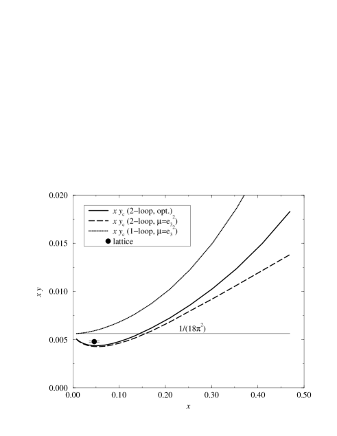
Figure 2: The quantity $x\times y_{c}(x)$ computed perturbatively for the U(1)+Higgs theory to different accuracies. The horizontal line is the leading $x\to 0$ result in eq. (3.4). The lattice Monte Carlo point for $x=0.0463$ is also shown. For $x=2$ perturbation theory is meaningless; then the lattice number is $x\times y_{c}(x=2)\approx-0.10$.

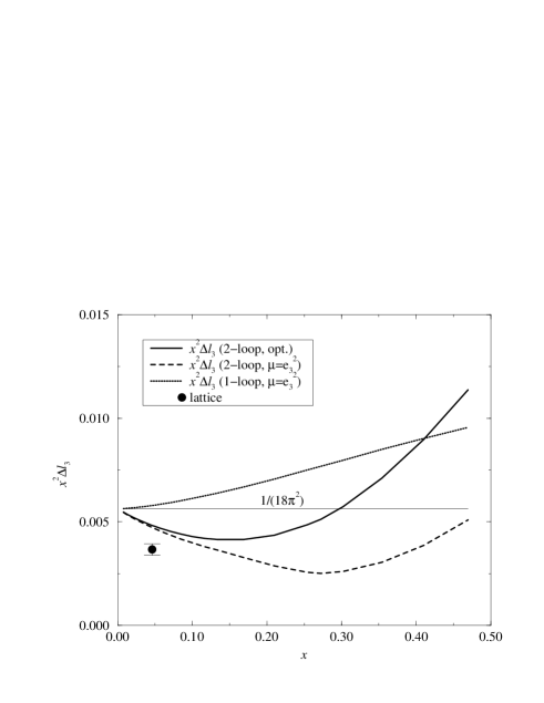
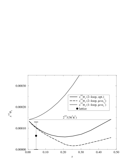
Figure 3: The same as Fig. 2 but for the jump of the order parameter ($\times x^{2}$) and for the interface tension ($\times x^{5/2}$).

4 U(1)+Higgs theory on the lattice

Our aim is to study the continuum theory in eq. (2.2) and it is thus crucial to keep the continuum variables $y,x$ fixed when discretizing the theory. This point has to do with ultraviolet renormalisation. The linear and logarithmic mass divergences are renormalised in the continuum theory in the $\overline{\mbox{\rm MS}}$ scheme. Discretization in itself is another scheme. The two schemes now have to be related so that correlators measured in the lattice scheme go to the correct continuum ones at given $y,x$ in the limit that the lattice spacing $a$ goes to zero. This computation has been carried out in [54–56]; for order ${\cal O}(a)$ corrections, see [57].

To discretize, we use the compact formulation of the gauge field and introduce the link field $U_{i}(\mbox{\bf x})=\exp[iae_{3}A_{i}(\mbox{\bf x})]\equiv\exp[i\alpha_{i}(\mbox{\bf x})]$. Rescaling the continuum scalar field to a dimensionless lattice field by

$$\phi^{*}\phi\to\beta_{H}\phi^{*}\phi/2a,$$ (4.1)

the lattice action becomes

$$S = \beta_{G}\!\!\sum_{\mbox{\bf x},i<j}\Bigl{[}1-\cos\hat{F}_{ij}(\mbox{\bf x})\Bigr{]}-\beta_{H}\sum_{\mbox{\bf x},i}{\mbox{Re}}\,\phi^{*}(\mbox{\bf x})U_{i}(\mbox{\bf x})\phi(\mbox{\bf x}+\hat{i})$$ (4.2)

$$+\sum_{\mbox{\bf x}}\phi^{*}(\mbox{\bf x})\phi(\mbox{\bf x})+\beta_{R}\sum_{\mbox{\bf x}}\left[\phi^{*}(\mbox{\bf x})\phi(\mbox{\bf x})-1\right]^{2},$$

where $\beta_{G}=1/e_{3}^{2}a$,

$$\hat{F}_{ij}(\mbox{\bf x})=\alpha_{i}(\mbox{\bf x})+\alpha_{j}(\mbox{\bf x}+\hat{i})-\alpha_{i}(\mbox{\bf x}+\hat{j})-\alpha_{j}(\mbox{\bf x}),$$ (4.3)

and a specific, customary choice has been made for $\beta_{H}$ (other choices are possible as well; see [38] for the action before any choice has been made). With these conventions, the lattice couplings $\beta_{G},\beta_{H},\beta_{R}$ are determined from [55, 56]

$$\beta_{G}={1\over e_{3}^{2}a},\qquad\beta_{R}={x\beta_{H}^{2}\over 4\beta_{G}},$$ (4.4)

$$2\beta_{G}^{2}\left({1\over\beta_{H}}-3-{x\beta_{H}\over 2\beta_{G}}\right)=y-{3.1759115(1+2x)\beta_{G}\over 2\pi}$$ (4.5)

$$\hskip 56.9055pt-{1\over 16\pi^{2}}\left[(-4+8x-8x^{2})(\log 6\beta_{G}+0.09)+25.5+4.6x\right].$$

Thus for a given continuum theory depending on one scale $e_{3}^{2}$ and the two dimensionless parameters $y,x$, the use of a lattice introduces a regulator scale $a$, and eqs. (4.2)–(4.5) specify, up to terms of order $e_{3}^{2}a$ [57], the corresponding lattice action.

In a non-compact formulation of the gauge field one would replace $1-\cos\hat{F}_{ij}\to\hat{F}_{ij}^{2}/2$ in eq. (4.2). Then the coefficient 25.5 in eq. (4.5) should be replaced with -1.1 [56].

An important quantity we will study is the scalar condensate $\langle\phi^{*}\phi\rangle$. In perturbation theory this has a linear and a logarithmic divergence and renormalisation induces a known logarithmic scale dependence $\langle\phi^{*}\phi(\mu)\rangle$ [54]. The condensate itself is not a physical quantity, only its changes are. The relation between the continuum (at the scale $\mu=e_{3}^{2}$) and lattice condensates is [56]

$${\langle\phi^{*}\phi(e_{3}^{2})\rangle_{\mbox{\scriptsize cont}}\over e_{3}^{2}}={\frac{1}{2}}\beta_{H}\beta_{G}\langle\phi^{*}\phi\rangle_{\mbox{\scriptsize latt}}-{3.1759115\beta_{G}\over 4\pi}-{1\over 8\pi^{2}}\biggl{[}\log(6\beta_{G})+0.668\biggr{]},$$ (4.6)

where “latt” refers to the normalisation of the field in the lattice action (4.2). The first term here is the scaling in eq. (4.1), the second is the linear, and the third the logarithmic divergence. The discontinuity of $\langle\phi^{*}\phi(\mu)\rangle$ in a first order transition is free from these divergences, as they are just constants.

For mass measurements we use the discretized forms of the operators discussed in Sec. 2. The $0^{++}$ and $1^{-+}$ charge conjugation even “scalar” operators $\phi^{*}\phi$ and Re$\,\phi^{*}D_{i}\phi$ and the $1^{--}$ vector operators Im$\,\phi^{*}D_{i}\phi$ and $\epsilon_{ijk}F_{jk}$ are on the lattice represented by

$$S(\mbox{\bf x}) = \phi^{\ast}(\mbox{\bf x})\phi(\mbox{\bf x}),$$ (4.7)

$$S_{i}(\mbox{\bf x}) = \mathop{\rm Re}\phi^{\ast}(\mbox{\bf x})U_{i}(\mbox{\bf x})\phi(\mbox{\bf x}+\hat{i}),$$ (4.8)

$$V_{i}(\mbox{\bf x}) = \mathop{\rm Im}\phi^{\ast}(\mbox{\bf x})U_{i}(\mbox{\bf x})\phi(\mbox{\bf x}+\hat{i}),$$ (4.9)

$$\tilde{V}_{i}(\mbox{\bf x}) = {\frac{1}{2}}\epsilon_{ijk}\sin\hat{F}_{jk}(\mbox{\bf x}).$$ (4.10)

In the 4d case these operators have been used for mass measurements in [58, 59]. Note that other (higher dimensional) operators with the same quantum numbers could be considered as well, and a systematic way of finding out which combinations couple to the lowest physical mass states, is with the blocking and consequent diagonalization techniques discussed in Sec. 6.5. In practice, the masses are measured from plane-plane correlators instead of the local operators in eqs. (4.7)–(4.10) as discussed in [38], and the photon mass measurement requires an external momentum [60].

5 Photon in 3d theories

Various 3d continuum theories with a photon in the physical spectrum are listed in Table 1. Here we shall add to this list the U(1)+Higgs theory in the compact lattice formulation, eq. (4.2) and, for comparison, also the discretized pure U(1) gauge theory in the compact formulation. The situation with photons in these theories is as follows:

Theory	d.o.f.’s in	d.o.f.’s in	$\gamma$ in	$\gamma$ in
	symm. ph.	broken ph.	symm. ph.?	broken ph.?
U(1)+Higgs	$A_{i},\phi^{*},\phi$	$W_{i},H$	yes	no
	= 2+2	= 3+1
SU(2)+adj. Higgs	$A_{i}^{a},\phi_{a}$	$W_{i}^{\pm},A_{i},H$	no	yes$\to$no
[21, 9]	= 3$\cdot$2+3	= 2$\cdot$3+2+1
SU(2)$\times$U(1)+fund.	$A_{i}^{a},B_{i},\phi_{k}$	$W_{i}^{\pm},Z_{i}^{0},A_{i},H$	yes	yes
Higgs [28]	= 3$\cdot$2+2+4	= 3$\cdot$3+2+1

Table 1: 3d continuum theories with a massless photon. The 2nd and 3rd columns list and count the free field degrees of freedom in the action (with and without a shift to the broken minimum). The last columns express whether a massless photon really appears in the physical spectrum. For SU(2)+adjoint Higgs the perturbatively massless photon becomes massive through non-perturbative effects [50].

$\bullet$ In 3d SU(2)$\times$U(1)+fundamental Higgs theory there is a massless field, “photon”, in both the symmetric and broken phases. It is appears both perturbatively and non-perturbatively as a physical state [28]. In the symmetric phase the photon is represented by the hypercharge field, whereas in the broken phase the photon field is a linear combination of the hypercharge and SU(2) gauge fields. Because the photon is massless in both phases, the two phases cannot be distinguished by its value and the phase diagram can be smoothly connected.

$\bullet$ In 3d SU(2)+adjoint Higgs theory there is, perturbatively, a massless photon in the broken phase but not in the symmetric phase. This is since after symmetry breaking by $\phi^{a}=(0,0,v)$ there remains a compact U(1) invariance, related to rotations between the 1,2 components. On the tree level the photon could thus be used to distinguish the two phases and the phase diagram seems to be split into two disjoint regions. However, what happens non-perturbatively [48–51] is that the photon becomes massive due to monopole configurations. The physics of how a gas of monopoles induces a mass is familiar from that of Debye screening in a plasma: if there is a gas of electrons ($e,T,m_{e},n_{e}$) in a neutralising background, there is a plasma frequency $\omega_{p}^{2}=e^{2}n_{e}/(m_{e}\epsilon_{0})$ and a screening length proportional to the inverse of $\omega_{p}$, so that the static photon correlation length has become finite due to charge screening. Since the monopole charge is $\sim\hbar/g_{3}$, where $g_{3}$ is the non-abelian gauge coupling, one similarly obtains

$$m_{\gamma}^{2}\sim{1\over g_{3}^{2}}n_{\mbox{\scriptsize monopole}}.$$ (5.1)

One can further carry out a semiclassical computation [51] leading to an expression of the type (the exponent is here for $x=0$)

$$n_{\mbox{\scriptsize monopole}}\sim\exp\biggl{[}-{4\pi m_{W}\over g_{3}^{2}}\biggr{]}.$$ (5.2)

Here $m_{W}$ is the perturbative mass of the the states $W^{\pm}$ (Table 1), and one should keep in mind that they are actually not physical states (since they are charged). Anyway, the fundamental quantity is the photon mass in eq. (5.1) which can be non-zero and has to be measured numerically. This has been done in [21, 9] and the phase diagram has been shown to be smoothly connected.

$\bullet$ In 3d U(1)+Higgs theory or in pure U(1) gauge theory on the lattice in the compact formulation there also is a massive photon. A semiclassical computation for this Polyakov mass gives in the weak coupling limit $\beta_{G}\gg 1$ [45, 46]

$${m_{\gamma}^{P}}/{e_{3}^{2}}=\pi(2\beta_{G})^{3/2}\exp\biggl{[}-{3.176\pi\over 4}\beta_{G}\biggr{]}.$$ (5.3)

In the strong coupling limit of small $\beta_{G}$, on the other hand [46],

$${m_{\gamma}^{P}}/{e_{3}^{2}}\approx{\pi^{2}\over 2}\beta_{G}^{2}\log{2\over\beta_{G}}.$$ (5.4)

Hence even in the compact U(1)+Higgs case, the phase diagram is connected for all finite $e_{3}^{2}a=1/\beta_{G}$, and the phase transition only appears in the limit $\beta_{G}\to\infty$. Below we measure $m_{\gamma}$ explicitly with a series of finite $\beta_{G}$’s and verify this behaviour. Thus, the massless state which appears in perturbation theory in the symmetric phase remains there in the full non-perturbative case in the continuum limit, as well, dividing the phase diagram into two disjoint regions.

6 Simulations

In this Section we discuss the numerical results of our lattice simulations. In Sec. 6.1 we discuss the parameter values used, in Sec. 6.2 the location of the phase transition point, in Sec. 6.3 the latent heat of the transition, in Sec. 6.4 our estimates for the interface tension, in Sec. 6.5 mass measurements and in Sec. 6.6 critical exponents.

6.1 Parameter values

We want to focus our attention on two separate regions: that of small $x$ (eq. (2.4)), where perturbation theory is expected to work and the transition is of first order, and that of large $x$ [38], where perturbation theory breaks down. In terms of the original physical theories these would correspond to type I superconductors or small Higgs masses and to type II superconductors or large Higgs masses, respectively. Some guidance concerning the limiting value is obtained from the fact that for the other 3d theories studied [23, 21] the first order transition terminates at $x=x_{c}\sim 0.1...0.3$ and that $x=0.5$ is the tree-level limiting value between type I and II superconductors.

Since the study of this problem is rather demanding in computer resources, we have chosen for the simulations two values of $x$, $x=0.0463$ and $x=2$, corresponding to strongly type I and type II superconductors. When mapped to hot scalar electrodynamics, these correspond to $m_{H}=30,160$ GeV.

One of the most essential points of the present lattice simulations is that the aim is to obtain results for the continuum theory (2.2) at fixed $y,x$. The extrapolation to the continuum limit thus has to be carried out carefully: one first takes a fixed $a$ (fixed $\beta_{G}$, eq. (4.5)) and extrapolates to infinite volume $V\to\infty$, and then one extrapolates $a\to 0$. To estimate the required lattice sizes of $V=(Na)^{3}$ and of the lattice spacing $a$, one notes that the lattices must be big enough to contain all relevant correlation lengths, and fine enough so that all the relevant correlation lengths are longer than several lattice spacings. Consider a system with a typical correlation length $\xi$. Then, accordingly, one has to satisfy (on a periodic lattice) $a\ll\xi\ll Na/2$ or, in physical units,

$$e_{3}^{2}a=1/\beta_{G}\ll e_{3}^{2}\xi\ll N/(2\beta_{G}).$$ (6.1)

Thus we have a lower limit for $N$:

$$N\gg e_{3}^{2}\xi\cdot 2\beta_{G},$$ (6.2)

and a lower limit for $\beta_{G}$:

$$\beta_{G}\gg 1/e_{3}^{2}\xi.$$ (6.3)

Eq. (6.2) expresses quantitatively why it is difficult to approach the continuum limit $\beta_{G}\to\infty$: the lattice size $N$ must be increased simultaneously. We shall use $\beta_{G}\geq 4$ and find that typically $e_{3}^{2}\xi$ varies between 0.3 and 2. Our lattice sizes are thus chosen as $N=32,\ldots,64$. The lattices used are shown in Table 2

$x$	$\beta_{G}$	volumes
0.0463	4	$8^{2}\times 40$	$12^{2}\times 60$
		$16^{2}\times 80_{m}$
	6	$8^{2}\times 40$	$12^{2}\times 60$
		$16^{2}\times 80_{m}$	$24^{2}\times 90_{m}$	$32^{2}\times 90_{m}$
		$64^{2}\times 128$
	8	$12^{2}\times 60$	$16^{2}\times 80$
		$24^{2}\times 90_{m}$	$32^{2}\times 90_{m}$	$40^{2}\times 120_{m}$
	12	$16^{2}\times 80$	$24^{2}\times 90$	$32^{2}\times 90$
2	4	$32^{3}$	$48^{3}$	$60^{2}\times 120$

Table 2: The lattice sizes used for the simulations at the transition temperature for each ($x,\beta_{G}$)-pair. In all cases, several $\beta_{H}$-values were used around the transition point. Multicanonical simulations are marked with the subscript (_m).

For each lattice listed in Table 2 we have performed simulations with several values of $\beta_{H}$. Typically at $x=0.0463$ each lattice has 3-5 different values of $\beta_{H}$ and at $x=2$ somewhat more. For $x=0.0463$ where we expect to find a first order transition, the different values of $\beta_{H}$ are joined together with the Ferrenberg-Swendsen multihistogram method [61]. This was not done for the $x=2$ data. The total number of combined heat-bath/overrelaxation sweeps is between $50000$ and $150000$ for each $\beta_{H}$ value. The measurements were not performed after every sweep in all cases, so the statistical sample sizes range between $20000$ and $100000$.

In the first order regime one expects to find supercritical slowing down when one goes to large enough lattices. We find that for lattice sizes larger than $V/e_{3}^{6}\approx 300$ one has to use the multicanonical algorithm to ensure that a correct statistical sample is generated.

The simulations were carried out with a Cray C94 at the Finnish Center for Scientific Computing. The total amount of computer power used was about 2500 h of CPU time or about $4\times 10^{15}$ floating point operations $\approx$ 130 Mflops year.

6.2 The critical point

6.2.1 Type I, $x=0.0463$

In principle, if the lattice spacing is small enough, the critical point can be obtained directly from Monte Carlo data by observing where the mass of the lowest vector excitation $m_{\gamma}$ vanishes. However, in practice the mass measurements are rather demanding in the vicinity of the critical point, and if possible we prefer to work with local operators. There are no known gauge invariant local order parameters, so we use order parameter -like quantities, which display a discontinuity at the transition point. The actual operators used are $R^{2}\equiv\phi^{*}\phi$ and the hopping term

$$L\equiv{1\over 3}\sum_{i=1}^{3}\mbox{Re }\phi^{*}(x)U_{i}(x)\phi(x+\hat{i}),$$ (6.4)

averaged over the volume.

For each individual lattice and $(\beta_{G},x)$ pair we locate the pseudocritical point $\beta_{H,c}$ using several different methods:

1. “Equal weight” of the histogram $p$ of $R^{2}$.

2. “Equal weight” of the histogram $p$ of $L$.

3. Maximum of the susceptibility $\chi$ of $R^{2}$ .

4. Maximum of the susceptibility $\chi$ of $L$.

5. Minimum of the 4th order Binder cumulant $B$ of $L$.

We give the susceptibility in dimensionless units as

$$\chi_{R^{2}}=e_{3}^{2}V\left\langle(\overline{\phi^{*}\phi}-\langle\overline{\phi^{*}\phi}\rangle)^{2}\right\rangle=N^{3}{\beta_{H}^{2}\over 4\beta_{G}}\left\langle(\overline{R^{2}}-\langle\overline{R^{2}}\rangle)^{2}\right\rangle,$$ (6.5)

where the overbar denotes a volume average, $\overline{R^{2}}=N^{-3}\sum_{x}R^{2}(\mbox{\bf x})$. The Binder cumulant $B$ has the standard definition.

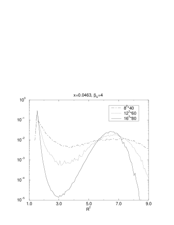
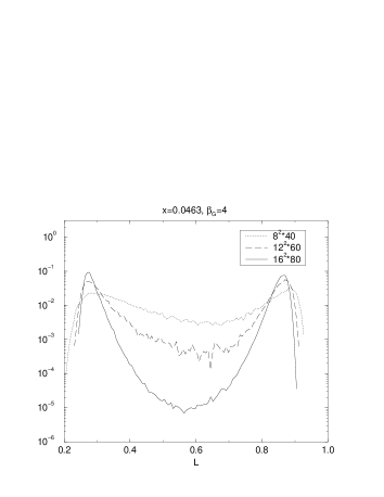
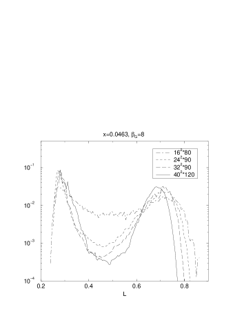
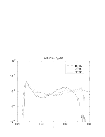
Figure 4: Equal weight histograms of $R^{2}$ and $L$ for $x=0.0463,\beta_{G}=4,6,8,12$. As the volume is increased the peaks remain at fixed positions as expected for a 1st order transition. For $\beta_{G}=12$ a proper $V\to\infty$ limit would necessitate larger lattices.

The equal weight histograms for $\beta_{G}=4,6,8,12$ are shown in Fig. 4. The histograms are obtained by joining all data together and then reweighting it to obtain the point where the areas of the two peaks are equal. This involves choosing a value to separate the two peaks. The choice is arbitrary, and introduces some systematic error to the determination of the critical point. We have used the same value for all lattices for a given $x,\beta_{G}$-pair. This value was determined by the minimum of the distribution in the largest volume. The error we quote is purely statistical: it was obtained by a jackknife analysis.

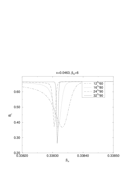
Figure 5: The susceptibility of $R^{2}$ divided by the volume $V$ (left) and the Binder cumulant of $L$ (right) at $x=0.0463,\beta_{G}=6$.

The locations of the maxima of the two susceptibilities and the minimum of the cumulant were also obtained by joining all data and then reweighting each jackknife block independently. As an example, the susceptibility of $R^{2}$ and the Binder cumulant of $L$ for $\beta_{G}=6$ are plotted in Fig. 5. The maxima of $\chi_{R^{2}}$ are plotted in Fig. 9.

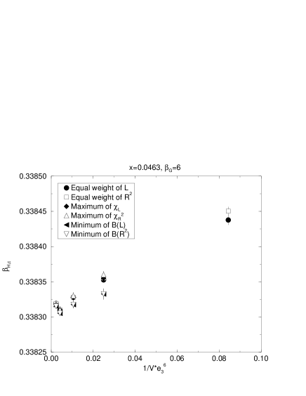
Figure 6: Different pseudocritical points for $x=0.0463,\beta_{G}=4,6,8,12$ as a function of the volume.

In Fig. 6 we have plotted different pseudocritical points for $x=0.0463,\beta_{G}=4\ldots 12$. The values obtained from different methods differ at a finite volume, but as one increases the volume these pseudocritical values come closer to each other and agree with each other at the infinite volume limit (within statistical errors). The results obtained from different methods are not statistically independent, but serve as a consistency check for the infinite volume extrapolation. The different pseudocritical points at the infinite volume limit are collected in Table 3.

$\beta_{G}$	$p(R^{2})$	$p(L)$	$\max\chi_{R}^{2}$	$\max\chi_{L}$	$\min B_{L}$
4	.3408199(18)	.3408208(19)	.3408208(25)	.3408192(28)	.3408189(34)
6	.3383148(07)	.3383151(06)	.3383073(37)	.3383111(24)	.3383075(23)
8	.3370630(10)	.3370630(10)	.3370629(16)	.3370639(23)	.3370638(23)
12	.3358169(40)	.3358165(40)	.3358314(107)	.3358235(92)	.3358069(86)

Table 3: The critical coupling $\beta_{H,c}$ extrapolated to infinite volume for all lattice spacings. The first two columns refer to the equal weight criterion.

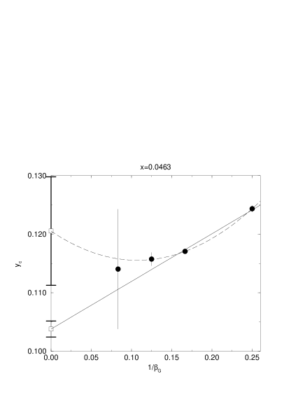
Figure 7: The infinite volume extrapolations of the pseudocritical points as a function of the lattice spacing $ae_{3}^{2}=1/\beta_{G}$. Quadratic and linear fits for the limit $a\to 0$ are also shown.

The extrapolation of $y_{c}$ to continuum is shown in Fig. 7. A linear extrapolation has a confidence level of $19\%$ and gives the value $y_{c}=0.1038(14)$. The quadratic fit gives $y_{c}=0.120(9)$. As the linear fit is reasonably good, we choose to quote that value as our continuum result. The 2-loop perturbative value $y_{c}=0.0947$ is more than $5\sigma$ from this.

It is possible to compare results at $\beta_{G}=4$ and $8$ to those obtained with non-compact simulations in [36]. We find that our critical couplings $\beta_{H,c}$ do not agree with the critical couplings obtained with noncompact simulations. From Fig. 5 in [36] one can read that the critical value for $\beta_{G}=4$ is roughly $0.34040$, with a very small error (smaller than $10^{-5}$). At $\beta_{G}=4$ we obtain $\beta_{H,c}=0.3408208(19)$, so the statistical error cannot explain this difference. This is not unexpected, as there is no need for the non-compact and compact results to agree at a finite lattice spacing. However, in the continuum limit one should obtain the same results. The authors of [36] choose to quote the critical temperature instead of the critical coupling $y_{c}$. If one extrapolates the results from [36] to continuum with a linear fit, one obtains $T_{c}=130.86(58)$. Using their eq. (13) one can try to compare our continuum value with this non-compact result. Our linear fit result corresponds to $T_{c}=131.28(4)$, so that the two results agree well in the continuum limit.

6.2.2 Type II: $x=2$

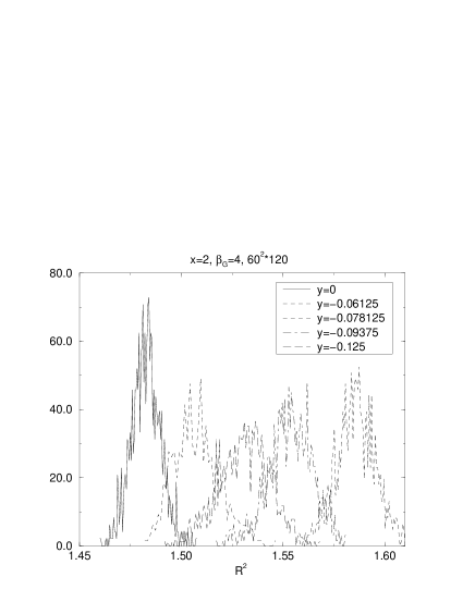
Figure 8: Histograms for $R^{2}$ at $x=2$, around the critical point $y\approx-0.05$. No two-peak structure is seen.

The location of the transition point in the type II regime has already been discussed in [38]. Measurements of averages of local operators in the type II regime show no evidence of discontinuities. Typical distributions are shown in Fig. 8. To quantify the effect, the maxima of the $R^{2}$ susceptibility are shown in Fig. 9 as a function of the volume. One can see that the maximum of $\chi_{R^{2}}$ remains constant. This finite size scaling behaviour is expected if there is no transition or if the transition is of second order with a critical exponent $\alpha\leq 0$. For understanding the type II regime and for quoting a definite value for $y_{c}$, mass measurements, especially that of $m_{\gamma}$, are required.

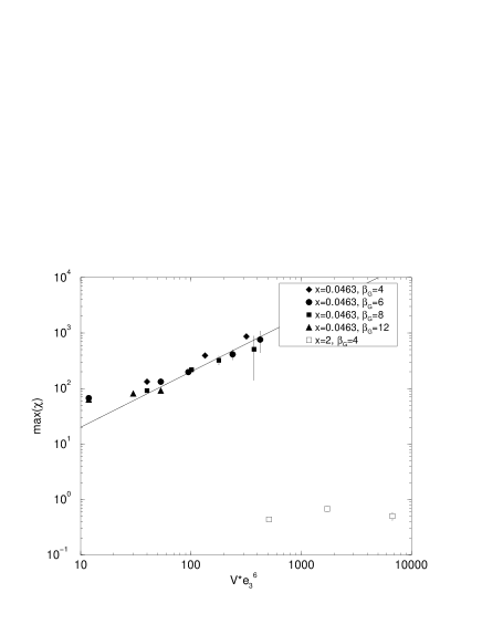
Figure 9: The maximum of the susceptibility of $R^{2}$ for $x=0.0463$ and $x=2$ as a function of the volume.

6.3 Latent heat

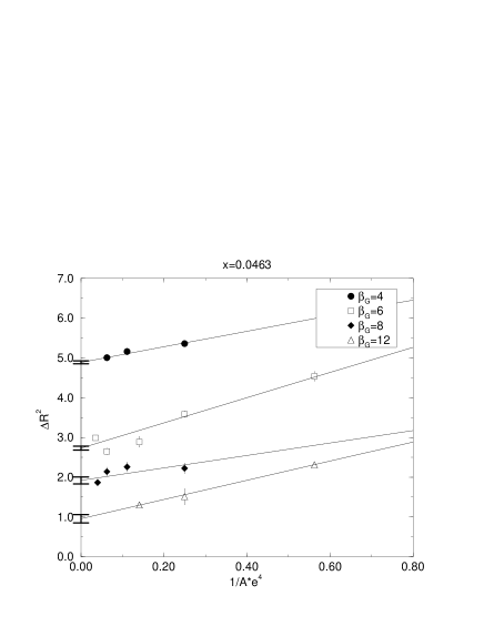
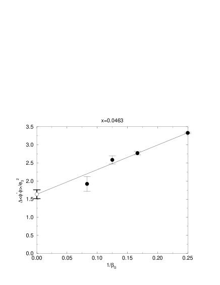
Figure 10: The infinite volume limits of $\Delta R^{2}$ (left) and the continuum limit of $\Delta\ell_{3}$ (right).

The latent heat — or the energy released in the transition — is directly proportional to $\Delta\ell_{3}=\Delta\left<\phi^{*}\phi\right>$ (see, e.g., Sec. 11 in [22]). This quantity is easily computed non-perturbatively from lattice simulations. In Fig. 10 we have plotted the infinite volume extrapolations of $\Delta\left<R^{2}\right>$. These can be converted to continuum values by eq. (4.1),

$${\Delta\left<\phi^{*}\phi\right>\over e_{3}^{2}}={1\over 2}\beta_{H}\beta_{G}\Delta\left<R^{2}\right>.$$ (6.6)

The infinite volume limit is taken by extrapolating linearly with the inverse area of the system, as extrapolation with the inverse volume would fail to accommodate the small differences between the different ratios of $N_{x}/N_{z}$.

The continuum limit of $\Delta\ell_{3}$ is displayed in Fig. 10. The continuum extrapolation is done with a linear fit, which seems to fit the data well – the confidence level of this fit is $28\%$. The final continuum value we obtain is $\Delta\ell_{3}/e_{3}^{2}=1.64(12)$, with a statistical error only.

Again the results should be compared with those obtained from perturbation theory and from non-compact lattice simulations. In [36] it was found that the value of $\Delta\ell_{3}$ increases with decreasing lattice spacing; however we find a rather strong decrease. Therefore, even though all our data except $\beta_{G}=12$ give a value higher than the perturbative one, our continuum value is considerably smaller than the perturbative value $\Delta\ell_{3}=2.25$. Taking into account the fact that our data at $\beta_{G}=12$ is of not as high quality as at smaller lattice spacings by using only the three largest lattice spacings for the continuum extrapolation, one still obtains a value smaller than the perturbative one, $\Delta\ell_{3}=1.71(13)$.

6.4 Interface tension

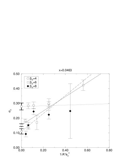
Figure 11: The infinite volume limit (left) and the extrapolated results at different lattice spacings (right) for the dimensionless interface tension $\sigma_{3}$. The systematic errors are expected to be much larger than the statistical ones shown in the figures.

The interface tension is the most difficult of the characteristics of the first order phase transition to measure. We estimate it with the histogram method [62]: at the critical point the system can reside in a mixed state consisting of domains of the pure phases. Because some extra free energy is associated with the interface separating the two phases, the area of the interface tends to a minimum and in a system with a geometry $N_{x}^{2}\times N_{z}$ (with $N_{z}>N_{x}$), the minimum area is just $2\times N_{x}^{2}a^{2}$ (due to periodic boundary conditions at least two interfaces are needed). Since the cost of an interface is $\sim\exp[-\sigma A/T]$, the dimensionless interface tension $\sigma_{3}$ can be calculated from

$$\sigma_{3}={1\over 2Ae_{3}^{4}}\log{P_{max}\over P_{min}},$$ (6.7)

where $P_{min}$ and $P_{max}$ are the minimum and the maximum of the probability distribution, and

$$e_{3}^{4}A=e_{3}^{4}N_{x}^{2}a^{2}=\left({N_{x}\over\beta_{G}}\right)^{2}.$$ (6.8)

For finite size corrections in the interface tension, see, e.g., [63].

The formula (6.7) requires that the two interfaces are far enough from each other so that their mutual interaction can be neglected. This would be signalled by a flat minimum in order parameter histograms, which should appear at large enough values of $N_{z}$. As seen from Fig. 4, a clearly flat minimum is not yet observed: the interfaces are so thick that their interaction is not negligible even for lattices of length 90. Thus non-negligible systematic errors are expected in our results.

The infinite volume extrapolations and the values obtained at different lattice spacings are shown in Figure 11. No extrapolation to continuum limit is performed even though the data seems to be consistent with a linear fit. This is since a linear fit would give a negative value for $\sigma_{3}$, which is unacceptable. We ascribe this unphysical behaviour to larger systematic errors at larger $\beta_{G}$’s, where the physical volume is not large enough to contain regions of clearly separated phases. The results we obtain are $\sigma_{3}=0.28(2)$ at $\beta_{G}=4$, $\sigma_{3}=0.15(1)$ at $\beta_{G}=6$, and $\sigma_{3}=0.09(2)$ at $\beta_{G}=8$; $\beta_{G}=12$ does not give a good enough signal for this purpose.

The perturbative value for $\sigma_{3}$ is 0.225, and as the results at $\beta_{G}=6$ and $8$ are both below this and the value seems to be decreasing with decreasing lattice spacing, one expects that the real value is significantly lower than the perturbative one. In Fig. 3 we have shown the conservative estimate $\sigma_{3}=0.14(14)$ which contains all the values we have measured.

6.5 Mass measurements

Since bulk quantities are rather insensitive to the phase transition at large values of $x$, we have paid special attention to mass (= inverse correlation length) measurements. Most of the results of our measurements have been reported in [38], and here we describe the techniques used in some more detail. There are several factors which could result in too high a value for a mass. First, one has to be sure that there is no contamination from higher excited states. This can be ensured by systematically searching for optimized operators coupling to the desired excitations, using blocking and diagonalization techniques. One also has to start the fits from sufficiently large values of $z$ and to monitor the behaviour of the effective mass. Second, one should use large enough lattices — in particular, one cannot expect to measure reliably masses smaller than $~{}\sim 1/N$.

6.5.1 Blocking

Figure 12: Effective masses at different blocking levels at $x=2,\beta_{G}=4$ as a function of $z$ (in lattice units).

To avoid having to use extremely large starting values of $z$ it is necessary to have a very good projection on the ground state. The projection can be improved upon by using blocking in the transverse direction [26, 64] both for the link variables $U_{i}(x)$,

$$U_{i}^{n+1}(x)={\frac{1}{3}}\biggl{[}U^{n}_{i}(x)U^{n}_{i}(x+\hat{i})+\sum_{j\neq i}U^{n}_{j}(x)U^{n}_{i}(x+\hat{j})U^{n}_{i}(x+\hat{j}+\hat{i})U^{n}_{j}(x+2\hat{i})^{-1}\biggr{]},$$ (6.9)

and for the scalar fields $\phi(x)$,

$$\phi^{n+1}(x)={\frac{1}{5}}\biggl{[}\phi^{n}(x)+\sum_{i=\pm 1}^{\pm 2}U^{n}_{i}(x)\phi^{n}(x+\hat{i})\biggr{]}.$$ (6.10)

The operators measured are then constructed from the blocked fields according to eqs. (4.7)–(4.10). The iteration level $n$ can be tuned for optimal overlap. In Fig. 12 we show the effect of blocking. Typically we find that the best results are obtained at blocking level 3 for all operators. The overlap of our blocked operators with the ground state ranged from being consistent with 100% far away from the critical point to 75% at the critical point.

6.5.2 Variational analysis

The blocking described above is in practice sufficient for the scalar excitations, where we are mostly interested in the ground state. However, we would like to know not only the ground state of the vector excitation but also have some information on the excited state. We are especially interested in knowing to what extent the lowest vector excitation couples to the operator $\tilde{V}_{3}$, which consists purely of gauge fields. To study this we have performed a variational analysis, which enables us to measure also the excited state.

Variational analysis is based on the fact that we have several operators which couple to the same quantum numbers. Even if each individual operator is not perfect in the sense that it also contains contributions from higher excited states, it should be possible to reduce this effect by suitably choosing linear combinations of individual operators. The basis that we use consists of different operators measured at different blocking levels. To be specific we use blocking levels 2 and 3; for scalar excitations we use the operators $\phi^{*}\phi$ and $\mbox{Re}\,\phi^{*}U_{i}\phi$ and for vector excitations $\mbox{Im}\,\phi^{*}U_{i}\phi$ and $\sin\hat{F}_{jk}$, see eqs. (4.7)–(4.10). Thus in both cases we have four different operators, which we call $O_{i}$. We then measure the whole $4\times 4$ cross correlation matrix

$$C_{ij}(z)=\left<O_{i}^{*}(z)O_{j}(0)\right>,$$ (6.11)

and then construct the improved operators ${\bf O_{i}}$ in the standard way [65],

$${\bf O_{i}}=\sum_{i}v^{i}_{k}O_{k}.$$ (6.12)

The operators are further normalised to unity at zero distance. The coefficients of the operator ${\bf O}_{1}$ for the ground state are found by maximising

$$\left<{\bf O_{1}}^{*}(a){\bf O_{1}}(0)\right>.$$ (6.13)

The operators for excited states can then be obtained by maximising the analogy of eq. (6.13) in a subspace that is orthogonal to the ground state operator ${\bf O}_{1}$.

We find that the variational analysis has usually little effect for the ground state — however, for excited states it is extremely helpful.

6.5.3 Fits

We extract the different masses by fitting exponentials to the corresponding correlation functions. In practice we have used one and two exponential fits and find that the difference between these two is within statistical errors. However, the one exponential fit is usually more stable, and therefore all numbers we quote are from one exponential fits.

One should note that the expectation values of the correlation function $C(z)$ are strongly correlated for close values of $z$. Typically the statistical correlation between $C(z)$ and $C(z+1)$ is greater than 95%. Therefore it is necessary to take this correlation into account when performing the fits. We find that the effect of taking this into account is to constrain the fits more tightly. The $\chi^{2}$ is increased and the variation between different jackknife blocks is decreased. If we do not use correlation information in our fits the fit parameters can fluctuate more freely causing not only unrealistically large errors but also changing the final value of the fit.

The major systematic error comes from the choice of the fitting range. We have carefully monitored the behaviour of the local mass, and start the fits only when a clear plateau is visible. Still changing the starting point by one or two lattice spacings changes the result; however as the change typically is roughly equal to the statistical error, we do not quote a systematic error on our fits. When interpreting the results one should bear in mind that it is possible that the systematic errors are at least as large as the statistical ones.

6.5.4 Polyakov mass

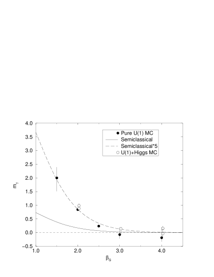
Figure 13: The photon mass as a function of $\beta_{G}$ in compact 3d U(1) gauge theory. The 5 $\times$ semiclassical curve extrapolates between weak and strong coupling regimes, and reproduces the non-perturbative values reasonably well for intermediate $\beta_{G}$.

Let us apply the methods described first to the photon mass in the compact formulation, see eqs. (5.3), (5.4). In order to use $m_{\gamma}$ as an order parameter, one has to be sure that this Polyakov mass it acquires at a finite lattice spacing, is negligible for all practical purposes. The semiclassical calculation (5.3) gives $m_{\gamma}/e_{3}^{2}=0.0033$ at $\beta_{G}=4$, which should be much smaller than anything we expect to be able to measure. However, as most of our conclusions depend strongly on $m_{\gamma}$, we have checked the validity of the semiclassical calculation by direct simulations in the pure U(1) gauge theory. We used a $24^{3}$ lattice, varied $\beta_{G}=1\ldots 4$ and used the operator (4.10) to measure $m_{\gamma}$.

The Monte Carlo results for pure gauge theory are shown in Fig. 13, together with the semiclassical result (5.3) and three data points in the U(1)+Higgs theory. The U(1)+Higgs data points were taken in the symmetric phase: we chose $x=2,y=0$ and $y=0.5$. One sees that adding the Higgs field does not affect the Polyakov mass, and that the Monte Carlo data agree with the semiclassical result for $\beta_{G}\mathop{\raise 1.29167pt\hbox{$>$\kern-7.5pt\raise-4.73611pt\hbox{$\sim$}}}3$ (in [47], agreement with semiclassical computations was found even at $\beta_{G}\sim 2$, but this relies on an “improved” $\beta_{G}$. Using that, the agreement in Fig. 13 is improved, as well). At $\beta_{G}=4$ the mass is clearly too small to be seen, and therefore can be neglected for all practical purposes. For lower values of $\beta_{G}$ we find that the formula $5\;\times$ semiclassical result reproduces the Monte Carlo data reasonably well, effectively interpolating between the strong and weak coupling results in eqs. (5.3), (5.4).

6.5.5 Masses

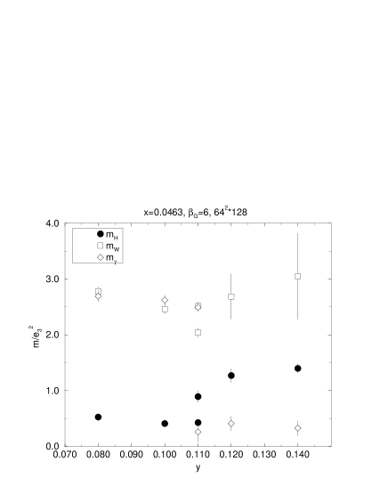
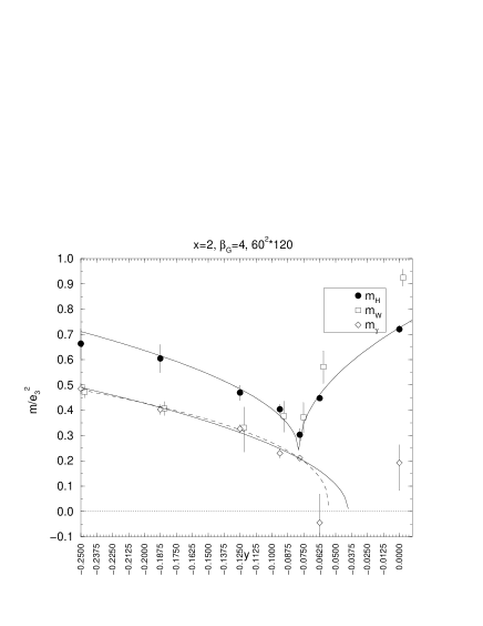
Figure 14: Masses near the critical point at $x=0.0463,\beta_{G}=6$ (left) and $x=2,\beta_{G}=4$ (right) (from [38]).

The masses in the U(1)+Higgs theory obtained with the methods described above are plotted in Fig. 14. We see that the mass of the photon vanishes within $2\sigma$ for both $x=0.0463$ and $x=2$ in the symmetric phase. When measured in $\sigma$’s, some of the results at $x=0.0463$ are somewhat further from zero. We believe that this due to the fact that no variational analysis was done for these points. Thus $m_{\gamma}$ serves as an order parameter for practical purposes.

The first order nature of the transition at $x=0.0463$ is clearly visible. All the masses show a clear discontinuity at $y_{c}(x)$. When going from the broken to the symmetric phase, $m_{H}$ jumps upwards (the scalar correlation length decreases from about 12$a$ to about 7$a$). The two vector excitations $m_{\gamma}$ and $m_{W}$, which were degenerate for $y<y_{c}$, separate so that $m_{\gamma}$ jumps to zero and $m_{W}$ becomes the mass of an excited two-scalar bound state.

At $x=2$ the pattern is less clear. The mass of the scalar excitation $m_{H}$ dips deeply, but does not go to zero. The value of $m_{H}$ at the minimum was also shown to be independent of the volume within statistical errors [38]. In the broken phase the two vector operators again see one single excitation, but in the symmetric phase $m_{\gamma}$ has dropped to zero and the other excitation has a large mass. However, on the basis of this data one cannot conclusively state what is happening. One can envisage the following possibilities:

• There is one line $y_{c}(x)$ on which $m_{\gamma}$ goes continuously to zero, $m_{H}$ has a minimum and $m_{\gamma},m_{W}$ separate.

• As the previous one but $m_{\gamma}$ jumps discontinuously to zero. This does not imply that the transition is of first order, as there is no jump in local quantities.

• The line $y_{c}(x)$ has split into several branches.

• All the masses go to zero at $y_{c}(x)$. This is the standard 2nd order scenario, which however, is not supported by our data.

The data shown is at fixed $\beta_{G}=4$ and one may ask whether the extrapolation to continuum would change the conclusions. The minimum of $m_{H}$ in Fig. 14 corresponds to a correlation length of 16$a$ and it is hard to see how making $a$ still smaller could change the results. We have made some runs at $\beta_{G}=3,6$ and did indeed not find any dependence outside of statistical errors.

6.6 Critical exponents

If $m_{\gamma}$ goes to zero continuously, one can measure its critical exponents. If the transition were of second order in the usual sense, there would be critical exponents for both scalar and vector correlation lengths:

$$m_{H} \sim |y-y_{c}|^{\nu_{H}},$$ (6.14)

$$m_{\gamma} \sim |y-yc|^{\nu}.$$ (6.15)

However, as we do not see any critical behaviour for the scalar correlation length, we cannot measure any critical exponent corresponding to it. The approximate scaling of $m_{H}$ away from the critical point has been discussed in [38].

To measure the critical exponent $\nu$ corresponding to a diverging photon correlation length, we have fitted functions of the form $m_{\gamma}/e_{3}^{2}=A(y_{c}-y)^{\nu}$ to the data shown in Fig. 14, both keeping the critical exponent $\nu$ fixed to the mean field value $0.5$ or allowing it to vary freely. We have also varied the range of $y$ which we include in the fits as $y_{min}=-1.25\ldots-0.25$. The fits with their confidence levels are shown in Table 4. We find that the critical point is rather stable, and that the value of the critical exponent is consistent with the mean field value. All the fits have rather low confidence levels, but as noted previously the errors we quote for masses are statistical only. Inclusion of the systematical errors (which we estimate to be of the same order of magnitude as the statistical errors) should bring the confidence levels to perfectly acceptable values.

In principle one could also measure the anomalous dimension $\eta_{N}$ of the photon correlation length, $\left<\tilde{V}_{3}(\mbox{\bf x})\tilde{V}_{3}(0)\right>\sim 1/|\mbox{\bf x}|^{1+\eta_{N}}$, but this would require a significantly extended analysis and more accurate data.

$y$ range	$A$	$y_{c}$	$\nu$	CL
$-0.25\ldots 0$	1.07(04)	-0.040(05)	0.5∗	0.14
$-0.25\ldots 0$	0.91(24)	-0.055(23)	0.39(17)	0.10
$-0.5\ldots 0.5$	0.995(19)	-0.033(04)	0.5∗	0.08
$-0.5\ldots 0.5$	0.931(62)	-0.048(13)	0.429(62)	0.07
$-1.25\ldots 0.5$	0.959(11)	-0.026(04)	0.5∗	0.006
$-1.25\ldots 0.5$	0.947(12)	-0.046(06)	0.440(19)	0.06

Table 4: Fits to determine the critical exponent $\nu$. The superscript (^∗) after a value means that it was kept fixed.

7 Conclusions

We have in this paper studied the 3d U(1)+Higgs model as an effective theory of various finite temperature theories. There are two separate aspects of the problem: computing the parameters of the effective theory in terms of the physical parameters of the full theory and studying the 3d theory as such. The first aspect has been solved for a very concrete physical phenomenon, superconductivity (Appendix A), and for a more academic system, hot scalar electrodynamics (Appendix B).

The second aspect, the study of the 3d theory as such, also splits into two parts: the region of first order transitions, corresponding to small $x=\lambda_{3}/e_{3}^{2}$ (type I superconductors, or small Higgs masses), and the region of possibly second order transitions, large $x$ (type II superconductors, or large $>m_{W}$ Higgs masses). The type II regime has been analysed in [38], and here we have mainly concentrated on the type I regime.

The evidence for a first order phase transition at $x=0.0463$ is compelling: several order parameter like quantities display a clear discontinuity, the finite volume scaling of the susceptibities is clearly consistent with a first order transition and the mass of the photon can be used as an effective order parameter. However, we have found that even when the transition is relatively strong, there are quantitatively some discrepancies with perturbation theory which seems to predict too strong a transition, see Fig. 3. This is in contrast to the case of the SU(2)+fundamental Higgs model, for example, where 2-loop perturbation theory works quite well for comparative Higgs masses [22]. The reason is probably just that the transition is weaker in U(1)+Higgs, but one might also speculate that physical topological defects (vortices) may play a role. In any case, the transition is too weak to be observed to be of first order in practical superconductor experiments.

At $x=2$ the situation is even more subtle. Many of the operators that can be used to study the phase transition at $x=0.0463$ do not display any indication of a transition at $x=2$. None of the local parameters ($R^{2}$ and $L$) show any discontinuity. The maxima of the susceptibilities remain constant. The scalar correlation length increases, but still seems to remain finite when extrapolated to infinite volume and zero lattice spacing [38]. The only indication of the transition is a vector correlation length diverging within statistical errors.

One thing to be checked in this argument is the use of the compact formulation which, in fact, makes the photon massive at a finite lattice spacing, if only by an exponentially small amount. Thus in a strict sense the transition vanishes altogether for a finite $a$. We have therefore studied the topological effects related to the compact formulation and demonstrated that they behave as expected, vanishing rapidly when approaching the continuum limit. Thus we believe that they do not alter the pattern described above.

The precise properties of the transition at $x=2$ remain unclear. Our data cannot distinguish between a second order phase transition in which the mass of the photon vanishes continuously and a more exotic scenario in which the photon mass has a discontinuity. To solve this unambiguously one would clearly need much more data. Another study requiring even more data would be that of the endpoint $x_{c}$ of the first order regime.

Because of the non-abelian gauge structure one might have expected computations in 3d SU(2)+Higgs theories [10,22–28] to be more complicated than those in U(1)+Higgs theories. However, just the opposite is the case. U(1)+Higgs is more demanding to simulate than SU(2)+Higgs at least in the compact formulation, as some of the correlation lengths are larger, the transition is weaker, the structure of the phase diagram is more complicated, and very large lattices are needed. This is analoguous, say, to what happens in the $q$-state Potts model in which the strength of the transition rapidly increases with the number $q$ of field components. Perhaps also the formation of physical topological defects, viz. vortices, plays a role in U(1)+Higgs.

Appendix Appendix  A: Full theory I: BCS superconductivity and the Ginzburg-Landau model

So far we have only treated the 3d effective theory as such; in these two Appendices we shall quantitatively discuss how two different physical theories map to the same effective theory. The first case is superconductivity.

Quantum phenomena in superconductors are microscopically described by the BCS theory [66]. In the normal state electrons do not form bound coherent states because of the repulsive Coulomb force but at low temperatures the electrons can form Cooper pairs due to their interaction with the ionic lattice. The electron-phonon interaction is important only at temperatures where the thermal excitations from the Fermi energy of the electron gas have an energy smaller than the average phonon energy. When this condition is satisfied the Fermi sea becomes unstable against the formation of bound pairs of electrons from states above the Fermi surface.

When the BCS theory is treated within the framework of the Green’s functions method one can find the connection between the microscopic BCS theory and the effective macroscopic Ginzburg-Landau model of superconductivity. Using the electron-electron interaction of the BCS theory and solving the equations of motion of the Hamiltonian Gor’kov [67] derived an equation describing the free energy density of Cooper pairs (we keep here $c,\hbar$):

$$f({\mbox{\bf x}}) = N(0)\bigg{[}r\xi_{0}^{2}\left|\left(\nabla-i\frac{2e}{\hbar c}A_{i}\right)\Delta({\mbox{\bf x}})\right|^{2}+$$ (A.1)

$$\quad+\left(\frac{T}{T_{0}}-1\right)|\Delta({\mbox{\bf x}})|^{2}+\frac{7\zeta(3)}{8(\pi T_{c})^{2}}|\Delta({\mbox{\bf x}})|^{4}\bigg{]},$$

where $\Delta({\mbox{\bf x}})=\langle\psi_{\uparrow}({\mbox{\bf x}})\psi_{\downarrow}({\mbox{\bf x}})\rangle$, $r\leq 1$ (=1 for perfect crystals) is an impurity parameter of the material,

$$\xi_{0}=\sqrt{\frac{7\zeta(3)}{48}}\frac{\hbar v_{F}}{\pi T_{c}}$$ (A.2)

sets the typical length scale of the system, and

$$N(0)=\frac{m^{2}v_{F}}{2\pi^{2}\hbar^{3}}$$ (A.3)

is the density of states at the Fermi surface. Note that the temperature parameter $T_{0}$ equals $T_{c}$ only on the mean field level. The connection between the free energy density (A.1) and the parameters in eq. (2.4) of the U(1)+Higgs theory can now be established by scaling the fields so that (A.1) has the form in eq. (2.2). The final relation becomes

$$y=\frac{1}{rq^{4}}\left(\frac{T}{T_{0}}-1\right),\,\,\,\,x=\frac{g}{(rq)^{2}},$$ (A.4)

where we have used the notations of [1]:

$$g=\frac{3T_{c}}{N(0)\hbar^{2}v_{F}^{2}\xi_{0}}=\sqrt{\frac{108\pi^{6}}{7\zeta(3)}}\left(\frac{T_{c}}{T_{F}}\right)^{2},$$

$$q=\frac{2e}{\hbar c}\sqrt{T_{c}\xi_{0}}=\sqrt{\frac{4e^{2}}{\hbar c\pi}\sqrt{\frac{7\zeta(3)}{48}}}\sqrt{v_{F}\over c},$$ (A.5)

with $T_{F}=mv_{F}^{2}/2\gg T_{c}$. What now is crucial is that widely different scales with large or small ratios appear. For low temperature superconductors ($T_{c}\sim 1$ K), $T_{c}/T_{F}\sim 10^{-4}$ and the Fermi velocity is $v_{F}\sim(10^{-3}-10^{-2})c$. These lead to values $g\sim 10^{-6}$ and $q\sim 0.01$ resulting in $x\sim 0.01/r^{2}$. For usual superconductors thus $x\ll 1$. In contrast, for high temperature superconductors typically $x\gg 1$. This follows from measurements of the penetration depth and the coherence length and from the fact that $x$ is simply half the square of their ratio, so that $x<1/2$ describes type I superconductors and $x>1/2$ type II superconductors. It is interesting that the physically challenging case (high $T_{c}$ superconductors) just corresponds to the region in which the G-L model has a particularly subtle structure. It is so in the relativistic case (Appendix B), as well, that the large $x$ regime correponds to the most challenging domain of the physical theory: large Higgs masses.

The big dimensionless ratios also appear in the expression for $y$ in eq. (A.4). This implies that although $y_{c}(x)$ is of order one for small $x$, $T_{c}/T_{0}-1$ is extremely small, of the order of $q^{-4}\sim 10^{-8}$. This smallness follows not from the dynamics of the 3d theory, but from the relation of the full and effective theories.

Similar statements apply in the case of the latent heat $L$. In the effective theory, $L$ is essentially the jump $\Delta\ell_{3}$ in $\langle\phi^{*}\phi\rangle$ at the phase transition point. For small $x$ (see eq. (3.6); now again $\hbar=c=1$),

$$\Delta\ell_{3}=\frac{1}{18\pi^{2}x^{2}}\approx\frac{r^{4}q^{4}}{18\pi^{2}g^{2}}.$$ (A.6)

The conversion into physical units [22] gives then

$$L=\Delta\ell_{3}e_{p}^{6}T_{c}^{5}\frac{dy}{dT}=T_{c}^{4}\frac{r^{3}e_{p}^{6}}{18\pi^{2}g^{2}}\simeq 1.15\times 10^{-18}K_{c}^{4}\frac{r^{3}e_{p}^{6}}{18\pi^{2}g^{2}}\mbox{J}/\mbox{cm}^{3},$$ (A.7)

where $e_{p}=2e=\sqrt{16\pi\alpha}\simeq 0.61$ is the coupling constant of the physical theory and $K_{c}$ is the transition temperature in Kelvins. For example, for Pb ($K_{c}=7.2$ K) the latent heat is

$$L\simeq 10^{-6}\mbox{J}/\mbox{cm}^{3}=10^{-5}\mbox{J}/\mbox{mole},$$ (A.8)

which is far too small to be detected experimentally at present. This is so in spite of the fact that the transition is quite strong from the point of view of the effective theory. Note also that non-perturbatively the transition is somewhat weaker than given by eq. (A.6), see Fig. 3, but this does not change the order of magnitude estimate in eq. (A.8).

Appendix Appendix  B: Full theory II: hot relativistic scalar + fermion electrodynamics

Secondly, we shall work out the 3d effective theory of finite $T$ relativistic scalar electrodynamics. Since we aim at precision, we here first have to discuss how the parameters of the Lagrangian are determined to 1-loop in the $\overline{\mbox{\rm MS}}$ scheme in terms of the measurable (in principle!) physical masses of the theory [13]. Next we have to relate this 4d finite $T$ theory and the 3d effective theory. This happens in two stages: first the momenta $p\mathop{\raise 1.29167pt\hbox{$>$\kern-7.5pt\raise-4.73611pt\hbox{$\sim$}}}\pi T$ (the superheavy modes) are integrated out, resulting in an effective bosonic 3d theory with fundamental and adjoint Higgs fields. Finally, the adjoint Higgs field (the heavy modes) is integrated out. Some parts of the latter two steps have been already discussed in [12, 29, 31]. The parametric accuracies of the effective theories derived have been discussed in [13].

B.1 Relation between physics and the Lagrangian in $\overline{\mbox{\rm MS}}$ in 4d

The Lagrangian of 4d scalar + chiral fermion electrodynamics is [68]

$${\cal L} = {\frac{1}{4}}F_{\mu\nu}F_{\mu\nu}+(D_{\mu}\phi)^{*}(D_{\mu}\phi)-\nu^{2}\phi^{*}\phi+\lambda(\phi^{*}\phi)^{2}$$ (B.1)

$$+\bar{\Psi}_{L}/\!\!\!\!{D}\Psi_{L}+\bar{\Psi}_{R}/\!\!\!{\partial}\Psi_{R}+g_{Y}\bar{\Psi}(\phi^{*}a_{L}+\phi a_{R})\Psi,$$

where

$$F_{\mu\nu}=\partial_{\mu}A_{\nu}-\partial_{\nu}A_{\mu},\quad D_{\mu}\phi=(\partial_{\mu}+ieA_{\mu})\phi,\quad/\!\!\!\!{D}\Psi_{L}=\gamma_{\mu}(\partial_{\mu}+ieA_{\mu})\Psi_{L},$$

$$\Psi_{R,L}=a_{R,L}\Psi,\quad a_{R,L}=(1\pm\gamma_{5})/2,\quad\phi=(\phi_{1}+i\phi_{2})/\sqrt{2}.$$ (B.2)

At the tree-level, the couplings $\nu^{2},\lambda,g_{Y}^{2}$ are related to the physical masses $m_{H}$, $m_{W}$ and $m_{t}$ of the $\phi_{1},A_{\mu}$, and $\Psi$ fields in the broken phase by

$$\nu^{2}=\frac{1}{2}m_{H}^{2},\quad\lambda=\frac{e^{2}}{2}\frac{m_{H}^{2}}{m_{W}^{2}},\quad g_{Y}^{2}=2e^{2}\frac{m_{t}^{2}}{m_{W}^{2}}.$$ (B.3)

The masses $m_{H}$, $m_{W}$, $m_{t}$ are analogous to the Higgs, W and top masses of the Standard Model, and they can, in principle, be experimentally determined. The gauge coupling $e^{2}$ is, in principle, determined in terms of some cross section.

When one takes into account loop corrections, the theory requires renormalization, and the relations in eq. (B.3) change. Let us for definiteness regularize the theory in the $\overline{\mbox{\rm MS}}$ scheme in $d=4-2\epsilon$ dimensions. At 1-loop level, the bare quantites are then related to the running renormalized quantities through

$$A_{B} = A(\mu)\biggl{[}1+\frac{\mu^{-2\epsilon}}{16\pi^{2}\epsilon}\Bigl{(}-e^{2}\frac{N_{s}+2N_{f}}{6}\Bigr{)}\biggr{]},$$ (B.4)

$$\phi_{B} = \phi(\mu)\biggl{[}1+\frac{\mu^{-2\epsilon}}{16\pi^{2}\epsilon}\Bigl{(}\frac{3e^{2}}{2}-\frac{g_{Y}^{2}}{2}\Bigr{)}\biggr{]},$$ (B.5)

$$\Psi_{B} = \Psi(\mu)\biggl{[}1+\frac{\mu^{-2\epsilon}}{16\pi^{2}\epsilon}\Bigl{(}-\frac{g_{Y}^{2}}{4}\Bigr{)}\biggr{]},$$ (B.6)

$$e_{B}^{2} = e^{2}(\mu)\biggl{[}1+\frac{\mu^{-2\epsilon}}{16\pi^{2}\epsilon}\Bigl{(}e^{2}\frac{N_{s}+2N_{f}}{3}\Bigr{)}\biggr{]},$$ (B.7)

$$\nu_{B}^{2} = \nu^{2}(\mu)\biggl{[}1+\frac{\mu^{-2\epsilon}}{16\pi^{2}\epsilon}\Bigl{(}-3e^{2}+4\lambda+g_{Y}^{2}\Bigr{)}\biggr{]},$$ (B.8)

$$\lambda_{B} = \lambda(\mu)+\frac{\mu^{-2\epsilon}}{16\pi^{2}\epsilon}\Bigl{(}3e^{4}-6\lambda e^{2}+10\lambda^{2}+2\lambda g_{Y}^{2}-g_{Y}^{4}\Bigr{)},$$ (B.9)

$$g_{Y,B}^{2} = g_{Y}^{2}(\mu)\biggl{[}1+\frac{\mu^{-2\epsilon}}{16\pi^{2}\epsilon}\Bigl{(}2g_{Y}^{2}-3e^{2}\Bigr{)}\biggr{]}.$$ (B.10)

Here $N_{s}=1$ is the number of scalar fields and $N_{f}=1$ is the number of fermion fields; $N_{s}$ and $N_{f}$ are used just to show the origin of the different contributions. The renormalized parameters of the theory run at 1-loop level as

$$\mu\frac{d}{d\mu}e^{2}(\mu) = \frac{\mu^{-2\epsilon}}{8\pi^{2}}\frac{e^{4}}{3}(N_{s}+2N_{f}),$$ (B.11)

$$\mu\frac{d}{d\mu}\nu^{2}(\mu) = \frac{\mu^{-2\epsilon}}{8\pi^{2}}(-3e^{2}+4\lambda+g_{Y}^{2})\nu^{2},$$ (B.12)

$$\mu\frac{d}{d\mu}\lambda(\mu) = \frac{\mu^{-2\epsilon}}{8\pi^{2}}(3e^{4}-6\lambda e^{2}+10\lambda^{2}+2\lambda g_{Y}^{2}-g_{Y}^{4}),$$ (B.13)

$$\mu\frac{d}{d\mu}g_{Y}^{2}(\mu) = \frac{\mu^{-2\epsilon}}{8\pi^{2}}(2g_{Y}^{4}-3e^{2}g_{Y}^{2}).$$ (B.14)

To relate the running parameters to the physical observables, one has to calculate suitable physical quantities to 1-loop order, and express the running parameters in terms of these. For illustration, let us consider relating the running parameter $\nu^{2}(\mu)$ to physical masses. To do so, we calculate the physical pole mass $m_{H}$ to 1-loop order. For the calculation, the field $\phi_{1}$ is shifted to the classical broken minimum $\phi_{c}=\nu^{2}/\lambda$. Then the radiatively corrected renormalized 1-loop propagator of the Higgs field is of the form

$$\langle\phi_{1}(-k)\phi_{1}(k)\rangle=\frac{1}{k^{2}+m_{1}^{2}-\Pi_{H}(k^{2},\mu)},$$ (B.15)

where $m_{1}^{2}=2\nu^{2}$. Solving for the pole $m_{H}$, one gets

$$\nu^{2}(\mu)=\frac{m_{H}^{2}}{2}\biggl{[}1+\frac{\Pi_{H}(-m_{H}^{2},\mu)}{m_{H}^{2}}\biggr{]}.$$ (B.16)

This expression is gauge-independent, since the self-energy is evaluated at the pole. The latter term in eq. (B.16) is the 1-loop correction to the tree-level formula in eq. (B.3), and contains the $\mu$-dependence in eq. (B.12).

To give the explicit form of the 1-loop expression for $\nu^{2}(\mu)$, we use the notation

$$h\equiv\frac{m_{H}}{m_{W}},\quad t\equiv\frac{m_{t}}{m_{W}}.$$ (B.17)

Inside 1-loop formulas, one may then write $\lambda=e^{2}h^{2}/2,\quad g_{Y}^{2}=2e^{2}t^{2}$. Let us also introduce the function

$$L_{1}(h)=-2\sqrt{4h^{-2}-1}\arctan\frac{1}{\sqrt{4h^{-2}-1}},$$ (B.18)

which has the special value $L_{1}(1)=-\pi/\sqrt{3}$. Then we get

$${\nu}^{2}(\mu) = \frac{m_{H}^{2}}{2}\biggl{\{}1+\frac{e^{2}}{16\pi^{2}}\biggl{[}(2h^{2}+2t^{2}-3)\ln\frac{\mu^{2}}{m_{W}^{2}}$$ (B.19)

$$-3h^{2}\ln h+\Bigl{(}7-\frac{3\sqrt{3}}{2}\pi\Bigr{)}h^{2}-5+\frac{6}{h^{2}}-4t^{2}\ln t+4t^{2}-8\frac{t^{4}}{h^{2}}$$

$$+\frac{h^{4}-4h^{2}+12}{2h^{2}}L_{1}(h)+2t^{2}\Bigl{(}1-4\frac{t^{2}}{h^{2}}\Bigr{)}L_{1}(h/t)\biggr{]}\biggr{\}}.$$

B.2 Integration over the superheavy scale

At high temperatures, the equilibrium thermodynamics of the theory defined byeq. (B.1) can be described by a superrenormalizable 3d effective field theory (for a review, see [69]). The Lagrangian of the effective theory is that in eq. (2.2) with a second scalar $A_{0}$:

$${\cal L}_{\rm eff} = \frac{1}{4}F_{ij}F_{ij}+(D_{i}\phi)^{*}(D_{i}\phi)+m_{3}^{2}\phi^{*}\phi+\lambda_{3}(\phi^{*}\phi)^{2}$$ (B.20)

$$+\frac{1}{2}(\partial_{i}A_{0})^{2}+\frac{1}{2}m_{D}^{2}A_{0}^{2}+\frac{1}{4}\lambda_{A}A_{0}^{4}+h_{3}\phi^{*}\phi A_{0}^{2},$$

where all the fields have the dimension GeV^1/2 and the couplings $e_{3}^{2},\lambda_{3},\lambda_{A},h_{3}$ have the dimension GeV.

The purpose of this section is to give the parameters $e_{3}^{2},h_{3},m_{3}^{2},\lambda_{3},m_{D}^{2},\lambda_{A}$ and the fields $A_{i},\phi$ in terms of the parameters in eq. (B.1), with the accuracy compatible with 1-loop renormalization of the vacuum theory, as described above. Apart from terms arising from fermions, the results have been given at 1-loop order in [12] (2-loop results for the mass parameters have been added in [31]). Here we add the effects of fermions. We use extensively the generic results from [13]. The basic notations are:

$$c=\frac{1}{2}\biggl{[}\ln\frac{8\pi}{9}+\frac{\zeta^{\prime}(2)}{\zeta(2)}-2\gamma_{E}]\approx-0.348725,$$

$$L_{b}(\mu)=2\ln\frac{\mu e^{\gamma_{E}}}{4\pi T}\approx 2\ln\frac{\mu}{7.0555T},\quad L_{f}(\mu)=2\ln\frac{\mu e^{\gamma_{E}}}{\pi T}\approx 2\ln\frac{\mu}{1.7639T}.\mbox{\hskip 28.45274pt}$$ (B.21)

Let us start with the relations of the wave functions. Using the ${\cal Z}^{\phi}$’s from eqs. (35–37) of [13], the momentum-dependent contribution of the superheavy modes to the two-point scalar correlator is

$${\cal Z}^{\phi}={\cal Z}^{\phi}_{\rm CT}-e^{2}{\cal Z}^{\phi}_{\rm SV}+\frac{1}{2}g_{Y}^{2}{\cal Z}^{\phi}_{\rm FF}.$$ (B.22)

For the spatial and temporal components of the gauge fields one gets

$${\cal Z}^{A}={\cal Z}^{A}_{\rm CT}-e^{2}{N_{s}}{\cal Z}^{A}_{\rm SS}-e^{2}N_{f}{\cal Z}^{A}_{\rm FF},$$ (B.23)

where the ${\cal Z}^{A}$’s are from eqs. (38–45) of [13]. Hence the wave functions in the 3d action are related to the renormalized 4d wave functions in the $\overline{\rm MS}$ scheme by

$$\phi_{3}^{2} = \frac{1}{T}\phi^{2}(\mu)\biggl{\{}1+\frac{1}{16\pi^{2}}\biggl{[}-3e^{2}L_{b}(\mu)+g_{Y}^{2}L_{f}(\mu)\biggr{]}\biggr{\}},$$ (B.24)

$$\bigl{(}A_{0}^{3d}\bigr{)}^{2} = \frac{1}{T}A_{0}^{2}(\mu)\biggl{\{}1+\frac{1}{16\pi^{2}}\frac{e^{2}}{3}\biggl{[}N_{s}L_{b}(\mu)+2N_{f}L_{f}(\mu)+2(N_{s}-N_{f})\biggr{]}\biggr{\}},$$ (B.25)

$$\bigl{(}A_{i}^{3d}\bigr{)}^{2} = \frac{1}{T}A_{i}^{2}(\mu)\biggl{\{}1+\frac{1}{16\pi^{2}}\frac{e^{2}}{3}\biggl{[}N_{s}L_{b}(\mu)+2N_{f}L_{f}(\mu)\biggr{]}\biggr{\}}.$$ (B.26)

The couplings $e_{3}^{2}$ and $h_{3}$ can be extracted from the superheavy contributions to the $(\phi\phi A_{i}A_{j})$- and $(\phi\phi A_{0}A_{0})$-correlators at vanishing external momenta, respectively. The contributions from the relevant diagrams are in eqs. (50–63) of [13]. The result is

$${\cal G}^{A}={\cal G}^{A}_{0}+{\cal G}^{A}_{\rm CT}-4\lambda e^{2}{\cal G}^{A}_{\rm SS}-4e^{4}{\cal G}^{A}_{\rm SV}+4\lambda e^{2}{\cal G}^{A}_{\rm SSS}-e^{2}g_{Y}^{2}{\cal G}^{A}_{\rm FFFF}.$$ (B.27)

When the fields are redefined according to eqs. (B.24)-(B.26) and the vertex is identified with the corresponding vertex in eq. (B.20), one gets

$$h_{3} = e^{2}(\mu)T\biggl{\{}1+\frac{1}{16\pi^{2}}\biggl{[}-\frac{e^{2}N_{s}}{3}L_{b}(\mu)-\frac{2e^{2}N_{f}}{3}L_{f}(\mu)+$$ (B.28)

$$\qquad\qquad\qquad+2e^{2}\Bigl{(}1+\frac{N_{f}-N_{s}}{3}\Bigr{)}+8\lambda-2g_{Y}^{2}\biggr{]}\biggr{\}},$$

$$e_{3}^{2} = e^{2}(\mu)T\biggl{\{}1+\frac{1}{16\pi^{2}}\biggl{[}-\frac{e^{2}N_{s}}{3}L_{b}(\mu)-\frac{2e^{2}N_{f}}{3}L_{f}(\mu)\biggr{]}\biggr{\}}.$$ (B.29)

For the scalar sector, the required correlators are most conveniently generated from the effective potential. With the Lagrangian masses

$$m_{1}^{2}=-\nu^{2}+3\lambda\phi^{2},\quad m_{2}^{2}=-\nu^{2}+\lambda\phi^{2},$$

$$m_{T}^{2}=e^{2}\phi^{2},\quad m_{f}^{2}=\frac{1}{2}g_{Y}^{2}\phi^{2},$$ (B.30)

the 1-loop (unresummed) contribution to the effective potential in Landau gauge is

$$V_{1}(\phi)={\cal C}_{S}(m_{1})+{\cal C}_{S}(m_{2})+{\cal C}_{V}(m_{T})+{\cal C}_{F}(m_{f}),$$ (B.31)

where the ${\cal C}$’s are from eqs. (69–71) of [13]. From the term quartic in masses in $V_{1}(\phi)$, one gets the superheavy contribution to the four-point scalar correlator at vanishing momenta. Redefining the field $\phi$ according to eq. (B.24), the coupling constant $\lambda_{3}$ is then

$$\lambda_{3} = T\biggl{\{}\lambda(\mu)+\frac{1}{16\pi^{2}}\biggl{[}\biggl{(}-3e^{4}+6\lambda e^{2}-10\lambda^{2}\biggr{)}L_{b}(\mu)+$$ (B.32)

$$\qquad\qquad+\biggl{(}g_{Y}^{4}-2\lambda g_{Y}^{2}\biggr{)}L_{f}(\mu)+2e^{4}\biggr{]}\biggr{\}}.$$

The coefficient of $\phi^{2}/2$ in $V_{1}(\phi)$ gives the 1-loop result for the scalar mass squared. The result is the term of order $g^{2}$ on the first line of eq. (B.36).

For the 2-loop contribution to the mass squared $m_{3}^{2}$, one needs the 2-loop effective potential $V_{2}(\phi)$. In terms of eqs. (81–93) of [13], the result is

$$V_{2}(\phi) = -\lambda^{2}\phi^{2}\Bigl{[}3{\cal D}_{\rm SSS}(m_{1},m_{1},m_{1})+{\cal D}_{\rm SSS}(m_{1},m_{2},m_{2})\Bigr{]}$$ (B.33)

$$-\frac{1}{2}e^{2}{\cal D}_{\rm SSV}(m_{1},m_{2},m_{T})-\frac{1}{4}e^{4}\phi^{2}{\cal D}_{\rm SVV}(m_{1},m_{T},m_{T})$$

$$-\frac{1}{4}g_{Y}^{2}\Bigl{[}{\cal D}_{\rm FFS}(m_{f},m_{f},m_{1})+{\cal D}_{\rm FFS}(m_{f},m_{f},m_{2})\Bigr{]}-\frac{N_{f}}{2}e^{2}{\cal D}_{\rm FFV}(m_{f},m_{f},m_{T})$$

$$-\frac{1}{4}\lambda\Bigl{[}3{\cal D}_{\rm SS}(m_{1},m_{1})+2{\cal D}_{\rm SS}(m_{1},m_{2})+3{\cal D}_{\rm SS}(m_{2},m_{2})\Bigr{]}$$

$$-\frac{1}{4}e^{2}\Bigl{[}{\cal D}_{\rm SV}(m_{1},m_{T})+{\cal D}_{\rm SV}(m_{2},m_{T})\Bigr{]}$$

$$+\frac{1}{2}{\cal D}_{\rm S}(m_{1})+\frac{1}{2}{\cal D}_{\rm S}(m_{2})+\frac{1}{2}{\cal D}_{\rm V}(m_{T})+{\cal D}_{\rm F}(m_{f}).$$

With the abbreviations

$$\tilde{\nu}^{2} = \nu^{2}(\mu)\biggl{\{}1+\frac{1}{16\pi^{2}}\biggl{[}3e^{2}L_{b}(\mu)-4\lambda L_{b}(\mu)-g_{Y}^{2}L_{f}(\mu)\biggr{]}\biggr{\}},$$ (B.34)

$$\tilde{g}_{Y}^{2} = Tg_{Y}^{2}(\mu)\biggl{\{}1+\frac{1}{16\pi^{2}}\biggl{[}3e^{2}L_{b}(\mu)-2g_{Y}^{2}L_{f}(\mu)-e^{2}(1+2\ln 2)+$$ (B.35)

$$\qquad\qquad\qquad+24\lambda\ln 2-4g_{Y}^{2}\ln 2\biggr{]}\biggr{\}},$$

the result for the 3d mass parameter is

$$m_{3}^{2}(\mu) = -\tilde{\nu}^{2}+T\biggl{(}\frac{1}{3}\lambda_{3}+\frac{1}{4}e_{3}^{2}+\frac{1}{12}\tilde{g}_{Y}^{2}\biggr{)}$$ (B.36)

$$+ \frac{T^{2}}{16\pi^{2}}\biggl{[}\frac{1}{18}e^{4}\biggl{(}N_{f}-16+18N_{f}\ln 2\biggr{)}+\frac{2}{3}\lambda e^{2}\biggr{]}$$

$$+ \frac{1}{16\pi^{2}}\biggl{(}-2h_{3}^{2}-4e_{3}^{4}+8\lambda_{3}e_{3}^{2}-8\lambda_{3}^{2}\biggr{)}\biggl{(}\ln\frac{3T}{\mu}+c\biggr{)}.$$

Here we have taken into account higher-order corrections on the last line, by replacing the 4d coupling constants by the 3d ones which appear in the exact running of $m_{3}^{2}(\mu)$ inside the superrenormalizable 3d theory.

The parameters $m_{D}^{2}$ and $\lambda_{A}$ require the calculation of the superheavy contributions on the $(A_{0}A_{0})$- and $(A_{0}A_{0}A_{0}A_{0})$-correlators at vanishing momenta. Using eqs. (96–101) of [13], the 1-loop 2-point correlator for the U(1)-field is

$${\cal A}^{(2)} = e^{2}\Bigl{[}2N_{s}{\cal A}^{(2)}_{\rm S}-N_{s}{\cal A}^{(2)}_{\rm SS}-N_{f}{\cal A}^{(2)}_{\rm FF}\Bigr{]}$$ (B.37)

and using eqs. (102–109) of [13], the four-point correlator is

$${\cal A}^{(4)}_{\rm SU(2)} = e^{4}\Bigl{[}-2N_{s}{\cal A}^{(4)}_{\rm SS}+4N_{s}{\cal A}^{(4)}_{\rm SSS}-N_{s}{\cal A}^{(4)}_{\rm SSSS}+N_{f}{\cal A}^{(4)}_{\rm FFFF}\Bigr{]}.$$ (B.38)

Since there is no tree-level term corresponding to the correlators in eqs. (B.37)-(B.38), the redefinition of fields in eq. (B.25) produces terms of higher order. The final results can then be read directly from eqs. (B.37)-(B.38):

$$m_{D}^{2} = \frac{e^{2}T^{2}}{6}(2N_{s}+N_{f}),$$ (B.39)

$$\lambda_{A} = \frac{e^{4}T}{6\pi^{2}}(N_{s}-N_{f}).$$ (B.40)

Apart from fermionic contributions, the 2-loop result for $m_{D}^{2}$ has been given in [31].

Using eqs. (B.11)-(B.14), one sees that the quantities $e_{3}^{2}$, $h_{3}$, $\lambda_{3}$, $\tilde{\nu}^{2}$ and $\tilde{g}_{Y}^{2}$ are independent of $\mu$ to the order they are presented above. In other words, when the running parameters $e^{2}(\mu)$, $\nu^{2}(\mu)$, $\lambda(\mu)$ and $g_{Y}^{2}(\mu)$ are expressed in terms of physical parameters, the $\mu$-dependence cancels in the 3d parameters. Note also that the bare mass parameter $m_{3}^{2}$ of the 3d theory is independent of $\mu$, so that one may use an independent renormalization scale inside the 3d theory.

B.3 Integration over the heavy scale

Consider now the parametric magnitude of the couplings in eq. (B.20). If we are interested in the study of the phase transition, we know this happens when $m_{3}^{2}(\mu)$ is very small and we see from eq. (B.36) that the tree-level term and the 1-loop term have to cancel so as to leave $m_{3}^{2}\sim e^{4}T^{2}$. At the same time the mass of $A_{0}$ is of the order of $eT$. The action in eq. (B.20) can then be further simplified by integrating out the $A_{0}$-field, leaving an action of the G-L form in eq. (2.2).

If we proceed from the $T\sim T_{c}$ region to $T\gg T_{c}$, eq. (B.36) implies that also $m_{3}$ is of the order of $eT$ and thus it should be integrated out together with $A_{0}$. The resulting theory is very simple: free electrodynamics in 3d. This is the statement that the magnetic sector of hot scalar ED is trivial.

For the case $T\sim T_{c}$ when the action is the one in eq. (2.2), we denote the new parameters by a bar. The relations of the old and the barred parameters have been given in [12], and we include the results here just for completeness.

The integration over the heavy scale proceeds in complete analogy with integration over the superheavy scale in Sec. B.2. Since there are no momentum-dependent 1-loop corrections to the $\phi_{3}$- and $A_{i}$-fields from the $A_{0}$-field, $\bar{\phi}_{3}=\phi_{3}$ and $\bar{A}_{i}=A_{i}^{3d}$. Since $A_{0}$ and $A_{i}$ do not interact, there are no 1-loop corrections to the $(\phi_{3})^{2}\bigl{(}A^{3d}_{i}\bigr{)}^{2}$-vertex, so that $\bar{e}_{3}=e_{3}$. The scalar self-couplings get modified, and at 1-loop order

$$\bar{\lambda}_{3}=\lambda_{3}-\frac{1}{8\pi}\frac{h_{3}^{2}}{m_{D}},\quad\bar{m}_{3}^{2}=m_{3}^{2}-\frac{1}{4\pi}h_{3}m_{D}.$$ (B.41)

To calculate the 2-loop corrections to the mass parameter, we use again the effective potential. The 2-loop contribution from the heavy scale to the effective potential is

$$V_{2}^{\rm heavy}(\phi)=\frac{1}{2}h_{3}\Bigl{[}D_{\rm LS}(m_{1})+D_{\rm LS}(m_{2})\Bigr{]}-h_{3}^{2}\phi^{2}D_{\rm LLS}(m_{1}),$$ (B.42)

where the $D$’s are from eqs. (119–122) of [13]. The mass parameter $\bar{m}_{3}^{2}(\mu)$ is then

$$\bar{m}_{3}^{2}(\mu) = -\tilde{\nu}^{2}+T\biggl{(}\frac{1}{3}\lambda_{3}+\frac{1}{4}e_{3}^{2}+\frac{1}{12}\tilde{g}_{Y}^{2}\biggr{)}-\frac{1}{4\pi}h_{3}m_{D}$$ (B.43)

$$\hskip 14.22636pt+\frac{T^{2}}{16\pi^{2}}\biggl{[}\frac{1}{18}e^{4}\biggl{(}N_{f}-16+18N_{f}\ln 2\biggr{)}+\frac{2}{3}\lambda e^{2}\biggr{]}$$

$$\hskip 14.22636pt+\frac{1}{16\pi^{2}}\biggl{[}\biggl{(}-2h_{3}^{2}\biggr{)}\biggl{(}\ln\frac{3T}{2m_{D}}+c+{\frac{1}{2}}\biggr{)}\biggr{]}$$

$$\hskip 14.22636pt+\frac{1}{16\pi^{2}}\biggl{(}-4\bar{e}_{3}^{4}+8\bar{\lambda}_{3}\bar{e}_{3}^{2}-8\bar{\lambda}_{3}^{2}\biggr{)}\biggl{(}\ln\frac{3T}{\mu}+c\biggr{)},$$

where we used eq. (B.36) and included higher order corrections on the last line, by replacing the couplings with those of the effective theory.

Using the results of this section for $\bar{m}_{3}^{2}(\mu)$ and $\bar{\lambda}_{3}$ and adding the running parameters from Sec. B.1, the final parameters $y$ and $x$ of the G-L action in eq. (2.2) are completely fixed in terms of the physical quantities $e^{2}$, the temperature $T$, and the physical pole masses $m_{W},m_{H}$ and $m_{t}$ at zero temperature. We do not write out the expressions explicitly. For illustration, let us show the final expression for $\tilde{\nu}^{2}$ from eqs. (B.19), (B.34):

$$\tilde{\nu}^{2} = \frac{m_{H}^{2}}{2}\biggl{\{}1+\frac{e^{2}}{16\pi^{2}}\biggl{[}2(3-2h^{2})\ln\frac{m_{W}e^{\gamma_{E}}}{4\pi T}-4t^{2}\ln\frac{m_{W}e^{\gamma_{E}}}{\pi T}$$ (B.44)

$$-3h^{2}\ln h+\Bigl{(}7-\frac{3\sqrt{3}}{2}\pi\Bigr{)}h^{2}-5+\frac{6}{h^{2}}-4t^{2}\ln t+4t^{2}-8\frac{t^{4}}{h^{2}}$$

$$+\frac{h^{4}-4h^{2}+12}{2h^{2}}L_{1}(h)+2t^{2}\Bigl{(}1-4\frac{t^{2}}{h^{2}}\Bigr{)}L_{1}(h/t)\biggr{]}\biggr{\}}.$$

References

- [1] H. Kleinert, Gauge Fields in Condensed Matter (World Scientific, 1989).
- [2] P.G. de Gennes, Solid State Commun. 10 (1972) 753; B.I. Halperin and T.C. Lubensky, ibid. 14 (1974) 997.
- [3] P. Ginsparg, Nucl. Phys. B 170 (1980) 388.
- [4] T. Appelquist and R. Pisarski, Phys. Rev. D 23 (1981) 2305.
- [5] S. Nadkarni, Phys. Rev. D 27 (1983) 917; Phys. Rev. D 38 (1988) 3287.
- [6] N.P. Landsman, Nucl. Phys. B 322 (1989) 498.
- [7] S.-Z. Huang and M. Lissia, Nucl. Phys. B 438 (1995) 54.
- [8] E. Braaten, Phys. Rev. Lett. 74 (1995) 2164; E. Braaten and A. Nieto, Phys. Rev. D 51 (1995) 6990; Phys. Rev. Lett. 76 (1996) 1417; Phys. Rev. D 53 (1996) 3421; A. Nieto, Int. J. Mod. Phys. A 12 (1997) 1431.
- [9] K. Kajantie, M. Laine, K. Rummukainen and M. Shaposhnikov, Nucl. Phys. B 503 (1997) 357 [hep-ph/9704416]; K. Kajantie, M. Laine, J. Peisa, A. Rajantie, K. Rummukainen and M. Shaposhnikov, Phys. Rev. Lett. 79 (1997) 3130 [hep-ph/9708207].
- [10] K. Kajantie, K. Rummukainen and M. Shaposhnikov, Nucl. Phys. B 407 (1993) 356.
- [11] A. Jakovác, K. Kajantie and A. Patkós, Phys. Rev. D 49 (1994) 6810; A. Jakovác and A. Patkós, Phys. Lett. B 334 (1994) 391; Nucl. Phys. B 494 (1997) 54.
- [12] K. Farakos, K. Kajantie, K. Rummukainen and M. Shaposhnikov, Nucl. Phys. B 425 (1994) 67 [hep-ph/9404201].
- [13] K. Kajantie, M. Laine, K. Rummukainen and M. Shaposhnikov, Nucl. Phys. B 458 (1996) 90 [hep-ph/9508379]; “High Temperature Dimensional Reduction and Parity Violation”, hep-ph/9710538.
- [14] M. Laine, Nucl. Phys. B 481 (1996) 43 [hep-ph/9605283].
- [15] J.M. Cline and K. Kainulainen, Nucl. Phys. B 482 (1996) 73 [hep-ph/9605235].
- [16] M. Losada, Phys. Rev. D 56 (1997) 2893 [hep-ph/9605266]; G.R. Farrar and M. Losada, Phys. Lett. B 406 (1997) 60 [hep-ph/9612346].
- [17] D. Bödeker, P. John, M. Laine and M. Schmidt, Nucl. Phys. B 497 (1997) 387 [hep-ph/9612364].
- [18] A. Rajantie, Nucl. Phys. B 501 (1997) 521 [hep-ph/9702255].
- [19] S. Nadkarni, Phys. Rev. Lett. 60 (1988) 491; Nucl. Phys. B 334 (1990) 559.
- [20] T. Reisz, Z. Phys. C 53 (1992) 169; P. Lacock, D.E. Miller and T. Reisz, Nucl. Phys. B 369 (1992) 501; L. Kärkkäinen, P. Lacock, D.E. Miller, B. Petersson and T. Reisz, Phys. Lett. B 282 (1992) 121; L. Kärkkäinen, P. Lacock, B. Petersson and T. Reisz, Nucl. Phys. B 395 (1993) 733; L. Kärkkäinen, P. Lacock, D.E. Miller, B. Petersson and T. Reisz, Nucl. Phys. B 418 (1994) 3.
- [21] A. Hart, O. Philipsen, J.D. Stack and M. Teper, Phys. Lett. B 396 (1997) 217 [hep-lat/9612021].
- [22] K. Kajantie, M. Laine, K. Rummukainen and M. Shaposhnikov, Nucl. Phys. B 466 (1996) 189 [hep-lat/9510020].
- [23] K. Kajantie, M. Laine, K. Rummukainen and M. Shaposhnikov, Phys. Rev. Lett. 77 (1996) 2887 [hep-ph/9605288].
- [24] E.-M. Ilgenfritz, J. Kripfganz, H. Perlt and A. Schiller, Phys. Lett. B 356 (1995) 561 [hep-lat/9506023]; M. Gürtler, E.-M. Ilgenfritz, J. Kripfganz, H. Perlt and A. Schiller, hep-lat/9512022; Nucl. Phys. B 483 (1997) 383 [hep-lat/9605042]; M. Gürtler, E.-M. Ilgenfritz and A. Schiller, UL-NTZ 08/97 [hep-lat/9702020]; UL-NTZ 10/97 [hep-lat/9704013].
- [25] F. Karsch, T. Neuhaus, A. Patkós and J. Rank, Nucl. Phys. B 474 (1996) 217 [hep-lat/9603004].
- [26] O. Philipsen, M. Teper and H. Wittig, Nucl. Phys. B 469 (1996) 445 [hep-lat/9602006]; “Scalar-gauge dynamics in 2+1 dimensions at small and large scalar couplings”, hep-lat/9709145
- [27] G.D. Moore and N. Turok, Phys. Rev. D 55 (1997) 6538.
- [28] K. Kajantie, M. Laine, K. Rummukainen and M. Shaposhnikov, Nucl. Phys. B 493 (1997) 413.
- [29] J.-P. Blaizot, E. Iancu and R.R. Parwani, Phys. Rev. D 52 (1995) 2543.
- [30] A. Jakovác, A. Patkós and P. Petreczky, Phys. Lett. B 367 (1996) 283 [hep-ph/9510230].
- [31] J.O. Andersen, Z. Phys. C 75 (1997) 147 [hep-ph/9606357]; hep-ph/9709294; hep-ph/9709418.
- [32] B.I. Halperin, T.C. Lubensky and S.-K. Ma, Phys. Rev. Lett. 32 (1974) 292.
- [33] C. Dasgupta and B.I. Halperin, Phys. Rev. Lett. 47 (1981) 1556.
- [34] J. Bartholomew, Phys. Rev. B 28 (1983) 5378.
- [35] Y. Munehisa, Phys. Lett. B 155 (1985) 159.
- [36] P. Dimopoulos, K. Farakos and G. Kotsoumbas, “Three-dimensional lattice U(1) gauge Higgs model at low ”, hep-lat/9703004.
- [37] M. Karjalainen and J. Peisa, Z. Phys. C 76 (1997) 319 [hep-lat/9607023].
- [38] K. Kajantie, M. Karjalainen, M. Laine and J. Peisa, Phys. Rev. B, in press [cond-mat/9704056].
- [39] H. Kleinert, Phys. Lett. A 93 (1982) 86; Lett. Nuovo Cimento 35 (1982) 405; M. Kiometzis, H. Kleinert and A.M.J. Schakel, Phys. Rev. Lett. 73 (1994) 1975; Fortschr. Phys. 43 (1995) 697; H. Kleinert and A.M.J. Schakel, supr-con/9606001; cond-mat/9702159.
- [40] A. Kovner, B. Rosenstein and D. Eliezer, Nucl. Phys. B 350 (1991) 325; A. Kovner, P. Kurzepa and B. Rosenstein, Mod. Phys. Lett. A 14 (1993) 1343.
- [41] J. March-Russell, Phys. Lett. B 296 (1992) 364.
- [42] W. Buchmüller and O. Philipsen, Phys. Lett. B 354 (1995) 403.
- [43] B. Bergerhoff, F. Freire, D.F. Litim, S. Lola and C. Wetterich, Phys. Rev. B 53 (1996) 5734.
- [44] I. Herbut and Z. Tešanović, Phys. Rev. Lett. 76 (1996) 4588; I.F. Herbut, J. Phys. A: Math. Gen. 30 (1997) 423 [cond-mat/9610052]; cond-mat/9702167.
- [45] T. Banks, R. Myers and J. Kogut, Nucl. Phys. B 129 (1977) 493.
- [46] J. Ambjørn, A. Hey and S. Otto, Nucl. Phys. B 210 (1982) 347.
- [47] R. Wensley and J. Stack, Phys. Rev. Lett. 63 (1989) 1764.
- [48] G. ’t Hooft, Nucl. Phys. B 79 (1974) 276.
- [49] A. Polyakov, JETP Lett. 20 (1974) 194.
- [50] A. Polyakov, Phys. Lett. B 59 (1975) 82; Nucl. Phys. B 120 (1977) 429; “Gauge Fields and Strings”, Ch. 4 (Harwood Academic Publishers, 1987).
- [51] M. Oleszczuk, “Mass generation in three dimensions”, hep-th/9412049.
- [52] W. Buchmüller, T. Helbig and D. Walliser, Nucl. Phys. B 407 (1993) 387.
- [53] A. Hebecker, Z. Phys. C 60 (1993) 271.
- [54] K. Farakos, K. Kajantie, K. Rummukainen and M. Shaposhnikov, Nucl. Phys. B 442 (1995) 317 [hep-lat/9412091]
- [55] M. Laine, Nucl. Phys. B 451 (1995) 484 [hep-lat/9504001].
- [56] M. Laine and A. Rajantie, Nucl. Phys. B, in press [hep-lat/9705003].
- [57] G.D. Moore, Nucl. Phys. B 493 (1997) 439; “O() errors in 3-D SU(N) Higgs theories”, hep-lat/9709053.
- [58] H.G. Evertz, K. Jansen, J. Jersák, C.B. Lang and T. Neuhaus, Nucl. Phys. B 285 (1987) 590.
- [59] B. Krishnan, U. Heller, V. Mitrjuskin and M. Müller-Preussker, “Compact U(1) lattice gauge-Higgs theory with monopole suppression”, hep-lat/9605043.
- [60] B. Berg and C. Panagiotakopoulos, Phys. Rev. Lett. 52 (1984) 94.
- [61] A.M. Ferrenberg and R.H. Swendsen, Phys. Rev. Lett. 61 (1988) 2635.
- [62] K. Binder, Phys. Rev. A 25 (1982) 1699.
- [63] Y. Iwasaki, K. Kanaya, L. Kärkkäinen, K. Rummukainen and T. Yoshié, Phys. Rev. D 49 (1994) 3540.
- [64] M. Teper, Phys. Lett. B 187 (1987) 345.
- [65] C.C. Fox, R. Gupta, O. Martin and S. Otto, Nucl. Phys. B 205 (1982) 188; B. Berg and A. Billoire, Nucl. Phys. B 221 (1983) 109; M. Lüscher and U. Wolff, Nucl. Phys. B 339 (1990) 222.
- [66] J. Bardeen, L.N. Cooper and J.R. Schrieffer, Phys. Rev. 108 (1957) 1175.
- [67] L.P. Gor’kov, Zh. Eksp. Fiz. 34 (1958) 735; Sov. Phys. JETP 7 (1958) 505; Zh. Eksp. Fiz. 36 (1959) 1918.
- [68] P. Arnold and O. Espinosa, Phys. Rev. D 47 (1993) 3546; Phys. Rev. D 50 (1994) 6662 (E).
- [69] M.E. Shaposhnikov, in Proceedings of the Summer School on Effective Theories and Fundamental Interactions, Erice, 1996 [CERN-TH-96-280, hep-ph/9610247].