A multigrid implementation of the Fourier acceleration method
for Landau gauge fixing
Abstract
We present a new implementation of the Fourier acceleration method for Landau gauge fixing. By means of a multigrid inversion we are able to avoid the use of the fast Fourier transform. This makes the method more flexible, and well suited for vector and parallel machines. We study the performance of this algorithm on serial and on parallel (APE100) machines for the 4-dimensional case. We find that our method is equivalent to the standard implementation of Fourier acceleration already on a serial machine, and that it parallelizes very efficiently: its computational cost shows a linear speedup with the number of processors. We have also implemented, on the parallel machines, a version of the method using conjugate gradient instead of multigrid. This leads to an algorithm that is efficient at intermediate lattice volumes.
Pacs numbers: 11.15.Ha, 02.60.Pn
I Introduction
Lattice gauge fixing is a necessary tool for understanding the relationship between continuum and lattice gauge theory. In fact, due to asymptotic freedom, the continuum limit of the lattice theory is the weak-coupling limit, and a weak-coupling expansion requires gauge fixing. Gauge fixing is also used in smearing techniques, and is necessary in order to evaluate quark/gluon matrix elements which can be used to extract non-perturbative results from Monte Carlo simulations [1]. It is therefore important to devise numerical algorithms to efficiently gauge fix a lattice configuration. An important issue regarding the efficiency of these algorithms is the problem of critical slowing-down (CSD), which occurs when the relaxation time of an algorithm diverges as the lattice volume is increased [2]. Conventional local algorithms have dynamic critical exponent , namely grows with the lattice side roughly as . Improved local methods show typically , while global methods may succeed in eliminating CSD completely, i.e. . Usually, global algorithms are more costly per iteration than local methods but, due to the elimination of CSD, their total computational cost becomes progressively lower than that of local methods at large lattice volumes. For this reason, efficient global algorithms are a highly desirable tool in large-volume applications. Another important issue is whether gauge-fixing algorithms can be implemented efficiently on parallel machines [3], since computers of this type are widely used in numerical studies of gauge theory on large lattices.
A well-known global approach for reducing CSD, applicable to gauge fixing as well as to other problems, is the method of Fourier acceleration (FA) [4]. The idea is to precondition a problem using a diagonal matrix in momentum space which is related to the solution of a simplified version of the problem [4, 5]. For the Landau gauge fixing case it can be proved [6] that Fourier acceleration eliminates CSD completely at infinite , namely the dynamic critical exponent is equal to zero; we have also obtained [7], at finite and in two dimensions, that is equal to . Moreover, the FA gauge-fixing method is very efficient in achieving a constant value for the longitudinal gluon propagator at zero three-momentum [6, 7, 8], which provides a very sensitive test of the goodness of the gauge fixing.
To fix Landau gauge on the lattice one looks for a minimum of the functional [9]
| (1) |
(We refer to [7] for notation.) The FA update is given by with
| (2) |
Here is a Fourier transform, is a tuning parameter, is the square of the lattice momentum, and is the lattice divergence of the gluon field . Thus, in this case, the preconditioning is obtained using in momentum space a diagonal matrix with elements given by (see [4, Section II] for details). The FA method in its original form makes use of the fast Fourier transform (FFT) to evaluate and , which requires a work of only where is the lattice volume [4], making it very appealing from the computational point of view. On the other hand, in order to implement FFT efficiently, one is restricted to using lattice sides that are powers of 2 [10, Chapter 12]. Moreover, implementing FFT on parallel machines of the SIMD type, and especially in 4 dimensions, can be very cumbersome [3, 11]. Here we present a new implementation of the FA method for Landau gauge fixing which avoids completely the use of the fast Fourier transform, and we test its performance for the -dimensional case on serial and on parallel machines. Preliminary results have been reported in [12].
II The multigrid FA method
Let us start by noting that the Fourier-mode decomposition in eq. (2) is equivalent to an inversion of the lattice Laplacian operator :
| (3) |
(Note that this inversion is carried out for each component of .) Thus, the FFT can be avoided by inverting using an alternative algorithm. Clearly, a good candidate should be suitable for use on parallel machines, and should require, ideally, the same computational work as FFT, i.e. . One such candidate is the multigrid (MG) algorithm with W-cycle and piecewise-constant interpolation. The idea of MG is to solve the lattice problem recursively, using local (Gauss-Seidel) updates on coarser versions of the original lattice in order to accelerate the convergence of slow modes of the solution. MG is an efficient iterative routine for inverting the Laplacian : with our choice of cycle and interpolation, each iteration of the method represents a work of order , and the number of iterations required for convergence is proportional to at most [13, 14]. Moreover, the MG routine can be successfully implemented on vector and parallel machines [15]. Thus this approach should preserve the property of eliminating CSD for Landau gauge fixing, while being applicable on parallel machines. At the same time, there is no restriction on the lattice size since, even for a fixed coarsening factor (e.g. 2), the size of the coarsest grid can be adjusted conveniently.
The overhead for the MG routine is likely to be larger than the one for FFT, but in our case it can be reduced by exploiting the fact that multigrid (as opposed to FFT) is an iterative method. For example, a significant computational gain can be obtained if one starts the inversion from a good initial guess for the solution. Also, by changing the stopping criterion for the inversion, the accuracy of the solution can be suitably varied, while for FFT the accuracy is fixed by the precision used in the numerical code. This is important since we will be tuning the parameter in eq. (2), and this tuning can be done only up to an accuracy of a few percent. Thus, the inversion of most likely will not require the high accuracy obtained in the FFT case, making possible a substantial reduction of the computational cost.
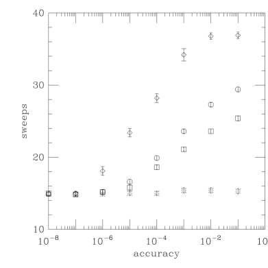
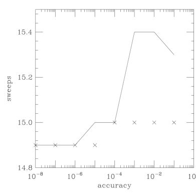
In order to test the feasibility of this approach we have started our simulations on a workstation, comparing the performance of the MG implementation of the Fourier acceleration method (MGFA) with the original implementation using FFT (which we call from now on FFTFA) [16]. As a first step, we tuned the parameter for the FFTFA method at infinite and . We obtained as optimal choice, and a number of gauge-fixing sweeps equal to . (Note that our data represent averages over a set of gauge configurations, and that our error bars are one standard deviation.) We then tested MGFA with : in addition to the W-cycle (where each grid is visited twice before proceeding to the next finer grid), we also tested for comparison the V-cycle (where each grid is visited once before proceeding to the next finer grid) and the standard Gauss-Seidel update; for the W-cycle we also varied the number of Gauss-Seidel relaxation sweeps on each grid (), and the minimum number of complete multigrid cycles (). Results for the number of gauge-fixing sweeps as a function of the accuracy [17], at infinite and , are reported in Fig. 1. By comparing these results with the result from the FFTFA method, it is clear that the number of gauge-fixing sweeps is independent of the method used for the inversion of , provided that a high enough accuracy is required. Among the tested versions of the MGFA method, the best from the point of view of computational cost is the one with the following choice of parameters: , an accuracy of about , two relaxation sweeps on each grid, and a minimum of two multigrid cycles for each inversion of . (We note that the CPU cost per iteration of this MG version is higher than for the other versions, but the fact that the inversion of the Laplacian can be stopped already at an accuracy of makes it the fastest version.) We then adopt this version of MG as the routine used for our MGFA method. For the MG routine we have chosen to use a coarsest grid of . Nevertheless we have checked that the performance of the chosen version does not change if a coarsest grid of is used. This is an important result, as we will see, for the implementation of the algorithm on parallel machines. We have also tested different initial guesses for the MG inversion, finding that the use of the solution to the previous inversion of the Laplacian is preferable to a null or random initial guess.
III Results and Conclusions
Initially, we have tested the performance of the MGFA method at and at on a workstation. The results, reported in Table I, are compared with those obtained for the FFTFA method and for the overrelaxation (OVE) algorithm [19], an improved local method which shows [6, 7] and which is often used for production runs in lattice gauge theory. In all cases the stopping criterion for the gauge fixing was . From the data at we can study the volume dependence of the computational cost for the various algorithms. Clearly, FFTFA and MGFA have a similar performance [20], showing a number of gauge-fixing sweeps increasing less than logarithmically with the volume , and the CPU time per sweep increasing roughly as . From our data we note that the number of MG cycles per inversion is essentially independent of the volume. As expected, for the overrelaxation algorithm the number of gauge-fixing sweeps is proportional to the lattice side , and the CPU time per sweep grows as the volume . The data for the total CPU time for the two implementations of the FA method and for the overrelaxation method are well fit by and , respectively. An extrapolation of our data using these fits predicts that either version of the FA method would be less costly than the overrelaxation method already at lattice side . Actually, the CPU cost for MGFA scales slightly better with the volume than for FFTFA. Thus, on a serial machine, and at , the fast Fourier transform can be successfully replaced by the MG routine, and MGFA should be the method of choice in the limit of large lattice volume. MGFA is equivalent to FFTFA also at and , and therefore it appears that the use of FFT can be avoided also at finite .
We remark that the FA method may have convergence problems at low values of [6, 21], probably related to the large number of local minima of the functional and/or to the existence of topological objects on the lattice. These problems are more likely to affect a global method than a local one (such as overrelaxation). A possible solution may be the smearing approach recently introduced in [22]: by smoothing out the lattice gauge configuration, one can perform gauge fixing at an effective close to infinity; this result is then used as a preconditioning of the original gauge-fixing problem, i.e. the gauge-fixing iterations start already close to a minimum. This approach aims at eliminating the problem of Gribov copies on the lattice, and is very well suited for the FA method. In fact, the two gauge-fixing steps involved (the one for the preconditioning — at high — and the one starting close to a minimum) are ideal applications of FA.
We then applied MGFA on two parallel (APE-Quadrics) machines of the APE100 series: the Q1 ( processors) and the QH4 ( processors) [23]. In order to implement the method on a parallel machine, the idea is to use as the coarsest grid for the MG routine a grid with volume equal to or larger than the number of processors. This avoids the problem of idle processors discussed in ref. [15]. For example, for the Q1 we implemented the MG routine with coarsest grid (respectively ) for the lattice volume (respectively ), while for the QH4 we used as the coarsest grid [24]. We have checked that the number of gauge-fixing sweeps does not change if we use for the MG routine an accuracy in the range –. This confirms the result obtained for a serial machine (see Fig. 1). In all our runs on APE machines we set the accuracy for the inversion to . Since these machines work in single precision we have also decreased the stopping criterion for the gauge fixing to .
As an alternative to the MG inversion, we have also implemented a version of the Fourier acceleration method in which the Laplacian is inverted using a standard (iterative) conjugate-gradient (CG) method. We call this method CGFA. The CG algorithm is simpler to program, and has been widely used on parallel machines. Its CPU time per cycle should be smaller than the one for MG, but the number of iterations required in order to achieve a fixed accuracy should increase faster than for the MG routine. In fact, we have checked that the number of multigrid iterations is essentially independent of the lattice volume, while the number of CG iterations grows roughly as .
In Table II we report the number of gauge-fixing sweeps obtained, at and for several lattice sizes, for the MGFA and the CGFA methods on APE machines. Their performances are compared with that of a standard overrelaxation (OVE) and with that of an unaccelerated local algorithm (the so-called Los Alamos algorithm, LOS) [6, 7]. These runs on parallel machines confirm that local algorithms are usually not able to achieve a constant value for the longitudinal gluon propagator at zero three-momentum. This can be checked by changing the stopping criterion for the gauge fixing: instead of considering we can consider the quantity defined in [6, 7], which monitors the fluctuations of this gluon propagator. Results are reported in Table II for the lattice volume . (Note that for LOS and OVE the results, in this case, have a large statistical error, due to the fact that for some configurations the gauge fixing did not converge within sweeps.)
Also in the parallel case, the FA method eliminates CSD at , and therefore should be the method of choice on large lattices. With respect to the overrelaxation method, the two implementations of FA are competitive already at volume if one requires a sensitive stopping criterion for the gauge fixing. We observe that, at our lattice sizes, the CG implementation is about two times faster than MGFA, but at large volumes we expect MGFA to win out.
We recall that local methods are more efficiently implemented on parallel machines than global ones, since they require smaller communication between processors. Global methods need implementations specifically designed for parallel machines in order to achieve a significant reduction of their computational overhead. For example, in a parallel implementation, the update for MG is not exactly of the Gauss-Seidel type, and in fact we observe that a higher (fixed) number of MG iterations is needed [25]. We think that our code for the MG routine can be optimized, since we have not explored more advanced features of MG that can play a role on parallel machines, such as asynchronous multigrid and the use of accommodative cycles instead of a fixed cycling strategy.
We have checked the dependence of the performance of the algorithms on the number of processors using the data from the Q1 and from the QH4, respectively for lattice volume and . The CPU time per gauge-fixing iteration per site scales down by a factor of approximately 62 for all the four algorithms, showing that the two FA methods parallelize as efficiently as the local ones. (Note that the number of processors increases by a factor 64 going from the Q1 to the QH4.)
We have shown that the fast Fourier transform in the Landau gauge-fixing Fourier acceleration method can be successfully substituted — on serial as well as on parallel machines — by an alternative inversion routine. This idea can in principle be extended to other applications of FA such as the case of quark propagators, and the Monte Carlo method for thermalization of lattice configurations.
Acknowledgements
Simulations were done on an IBM RS-6000/340 workstation at New York University, and on two APE-Quadrics machines at the University of Rome Tor Vergata. We wish to thank Philippe de Forcrand and Alan Sokal for helpful discussions.
REFERENCES
- [1] For a review see G.C.Rossi, Nucl.Phys. B (Proc.Suppl.) 53 (1997) 3.
- [2] See for example: U.Wolff, Nucl.Phys. B (Proc.Suppl.) 17 (1990) 93; A.D.Sokal, Nucl.Phys. B (Proc.Suppl.) 20 (1991) 55.
- [3] H.Suman and K.Schilling, Parallel Computing 20 (1994) 975.
- [4] C.T.H.Davies et al., Phys.Rev. D37 (1988) 1581.
- [5] G.G.Batrouni et al., Phys.Rev. D32 (1985) 2736; G.Katz, et al., Phys.Rev. D37 (1988) 1589; E.Dagotto and J.B.Kogut, Phys.Rev.Lett. 58 (1987) 299; E.Dagotto and J.B.Kogut, Nucl.Phys. B290 (1987) 451.
- [6] A.Cucchieri and T.Mendes, Nucl.Phys. B (Proc.Suppl.) 53 (1997) 811; A.Cucchieri and T.Mendes, in preparation.
- [7] A.Cucchieri and T.Mendes, Nucl.Phys. B471 (1996) 263.
- [8] P.Marenzoni, G.Martinelli and N.Stella, Nucl.Phys. B455 (1995) 339.
- [9] K.G.Wilson, Recent Developments in Gauge Theories Proc. NATO Advanced Study Institute (Carges̀e, 1979), eds. G. ’t Hooft et al. (Plenum Press, New York - London, 1980); J.E.Mandula and M.Ogilvie, Phys.Lett. B185 (1987) 127.
- [10] W.H.Press et al., Numerical Recipes in Fortran (Cambridge University Press, Cambridge, 1992, second edition).
- [11] Very recently, a new implementation of FFT for SIMD systems has been presented in Th.Lippert et al., hep-lat/9710060. The method is applied to a 2-dimensional case and could in principle be extended to 4 dimensions.
- [12] A.Cucchieri and T.Mendes, hep-lat/9710040, to appear in the Proc. of the Lattice 97 Conference.
- [13] For details of the implementation and for an introduction to the recursive (deterministic) MG method see for example Section II of J.Goodman and A.D.Sokal, Phys.Rev. D40 (1989) 2035 and references therein.
- [14] We note that we use here the MG routine inside the FA method, as an alternative way of dealing with the Fourier transforms in eq. (2). This should not be confused with the multigrid gauge-fixing method presented in: Ph. de Forcrand and R.Gupta, Nucl.Phys. B (Proc.Suppl.) 9 (1989) 516; A.Hulsebos, M.L.Laursen and J.Smit, Phys.Lett. B291 (1992) 431. In that case, multigrid is used directly in order to minimize . The method seems to reduce CSD significantly only if multigrid is combined with overrelaxation.
- [15] L.Stals, Parallel Implementation of Multigrid Methods, Proc. of the Sixth Biennial Conference on Computational Techniques and Applications (Canberra, 1993), eds. D.Stewart et al.
- [16] We have used single precision for the FFT and for the MG inversion routines, while for the gauge fixing we have used double precision.
- [17] Our definition of accuracy is , where is the residual at the -th iteration.
- [18] The tuning of was done independently for the MGFA and the FFTFA method. In all cases the optimal choice was the same. This result confirms that the use of a different routine for inverting the Laplacian does not modify the performance of the gauge-fixing algorithm, if a high enough accuracy is required for this inversion.
- [19] J.E.Mandula and M.Ogilvie, Phys.Lett. B248 (1990) 156.
- [20] We have chosen the version of the MG routine that provides us with the same number of gauge-fixing sweeps as for the FFTFA. In this way the critical behavior of the MGFA method is that of the FFTFA method (CSD almost completely eliminated). Alternatively, one could choose to require even less accuracy in the inversion of , which would imply a higher number of gauge fixing sweeps (see Fig. 1), but possibly with a lower total CPU cost. This would represent a modified MGFA method, with a different critical behavior, and it is not clear whether this method would show no CSD.
- [21] F.Gutbrod, A Study of the Gluon Propagator in Lattice Gauge Theory, DESY-96-252 preprint.
- [22] J.E.Hetrick and Ph. de Forcrand, hep-lat/9710003, to appear in the Proc. of the Lattice 97 Conference.
- [23] The Q1 has a peak performance of about Mflops and a total memory of Mbytes, while the QH4 has a peak performance of about Gflops and a total memory of Mbytes. Both machines work in standard single precision, and have a 3- torus topology.
- [24] On the coarsest grid, we have used Gauss-Seidel relaxation. In vector and parallel machine applications of multigrid one often uses a conjugate gradient algorithm to relax the solution on the coarsest grid [see for example S.Solomon and P.G.Lauwers, Proc. of the Workshop on Fermion Algorithms (Jul̈ich, 1991), 149]. In our case, even for our largest coarsest grid (), we do not see an effective gain with respect to the simple Gauss-Seidel update (see [12]).
- [25] We have checked that increasing the number of relaxation sweeps per grid causes a reduction of the total MG cycles needed per inversion, but does not lead to a computational gain.
| algorithm | GF sweeps | CPU time (s) | |||
|---|---|---|---|---|---|
| OVE | |||||
| FFTFA | |||||
| MGFA | |||||
| OVE | |||||
| FFTFA | |||||
| MGFA | |||||
| OVE | |||||
| FFTFA | |||||
| MGFA | |||||
| OVE | |||||
| FFTFA | |||||
| MGFA |
| algorithm | GF sweeps | CPU time (s) | ||
|---|---|---|---|---|
| LOS | 57.3 0.6 | |||
| OVE | 23.0 0.3 | |||
| CGFA | 13.9 0.1 | 4.56 0.07 | ||
| MGFA | 13.8 0.1 | 13.4 0.2 | ||
| LOS | 117 2 | 18.4 0.4 | ||
| OVE | 33.6 0.5 | 5.9 0.1 | ||
| CGFA | 16.4 0.3 | 34.1 0.7 | ||
| MGFA | 16.2 1.0 | 92 2 | ||
| LOS | 198 2 | |||
| OVE | 46.3 0.6 | |||
| CGFA | 17.6 0.2 | 2.12 0.04 | ||
| MGFA | 17.3 0.1 | 5.95 0.08 | ||
| LOS | 640 20 | 83 2 | ||
| OVE | 84 2 | 12.0 0.3 | ||
| CGFA | 21.5 0.7 | 49 1 | ||
| MGFA | 20.7 2.0 | 98 3 | ||
| LOS | 1970 90 | 553 30 | ||
| OVE | 252 70 | 75 20 | ||
| CGFA | 23.4 0.8 | 57 2 | ||
| MGFA | 22 3 | 123 3 |