Finite Lattice Hamiltonian Computations in the P-Representation: the Schwinger Model

Abstract

The Schwinger model is studied in a finite lattice by means of the P-representation. The vacuum energy, mass gap and chiral condensate are evaluated showing good agreement with the expected values in the continuum limit.

1 Introduction

A useful formulation of gauge theories, both from the conceptual and methodological point of view, is the one in terms of gauge invariant excitations or string-like objects. The so-called P-representation [1], consisting of a Hilbert space of path labeled states, has been used on the lattice to perform analytical Hamiltonian calculations. A cluster approximation allowed to provide qualitatively good results for the $(2+1)$ QED [2] and the $(3+1)$ QED [3] with staggered fermions. A description in terms of paths or strings, besides the general advantage of only involving gauge invariant excitations, is appealing because all the gauge invariant operators have a simple geometrical meaning when realized in the path space. However, the computational method implemented, up to now, on a formally infinite lattice, has the serious drawback of the explosive proliferation of clusters with the order of the approximation. In order to tackle this difficulty we propose in this paper to explore the previous method implemented now on a finite lattice. As a first test, we choose the simplest lattice gauge theory with dynamical fermions, the Schwinger model or (1+1) QED. This massless model can be exactly solved in the continuum and it is rich enough to share relevant features with 4-dimensional QCD as confinement or chiral symmetry breaking with an axial anomaly [4]. For this reason it has been extensively used as a laboratory to analyze the previous phenomena. The lattice Schwinger model also become a popular benchmark to test different techniques to handle dynamical fermions [5]-[6].

This article is organized into four sections. In section 2 we show the formulation of the model in the P-representation. The electric and interaction components of the Hamiltonian operator are realized in this basis of “electromeson” states. In section 3, first, we describe the finite lattice Hamiltonian approach. Second, we show the calculation of the ground-state energy, the mass gap and chiral condensate. These results are discussed in the concluding section.

2 Schwinger Model in the Lattice P-Representation

The P-representation offers a gauge invariant description of physical states in terms of kets $\mid P>$, where $P$ labels a set of connected paths $P_{x}^{y}$ with ends $x$ and $y$ in a lattice of spacing $a$. In the continuum, the connection between the P-representation and the ordinary representation (“configuration” representation), in terms of the fermion fields $\psi$ and the gauge fields $U_{\mu}(x)=\exp[ieaA_{\mu}(x)]$, can be performed considering the natural gauge invariant object constructed from them:

$$\Phi(P_{x}^{y})={\psi}^{\dagger}(x)U(P_{x}^{y})\psi(y),$$ (1)

where $U(P_{x}^{y})=\exp[ie\prod_{\ell\in P}A_{\ell}]$ ( $\ell\equiv(x,\mu)$ denote the links ).

The immediate problem we face is that $\Phi$ is not purely an object belonging to the “configuration” basis because it includes the canonical conjugate momentum of $\psi$, ${\psi}^{\dagger}$. The lattice offers a solution to this problem consisting in the decomposition of the fermionic degrees of freedom. Let us consider the Hilbert space of kets $\mid{\psi}_{u}^{\dagger},{\psi}_{d},A_{\mu}>$, where $u$ corresponds to the $up$ part of the Dirac spinor and $d$ to the $down$ part. Those kets are well defined in terms of “configuration” variables (the canonical conjugate momenta of ${\psi}_{d}$ and ${\psi}_{u}^{\dagger}$ are ${\psi}_{d}^{\dagger}$ and ${\psi}_{u}$ respectively.) Then, the internal product of one of such kets with one of the path dependent representation (characterized by a lattice path $P_{x}^{y}$ with ends $x$ and $y$) is given by

$$\Phi(P_{x}^{y})\equiv<P_{x;i}^{y;j}\mid{\psi}_{u}^{\dagger},{\psi}_{d},A_{\mu}>$$

$$={\psi}_{u;i}^{\dagger}(x)U(P_{x}^{y}){\psi}_{d;j}(y),$$ (2)

where $i$ and $j$ denote a component of the spinor $u$ and $d$ respectively. Thus, it seems that the choice of staggered fermions is the natural one in order to build the lattice P-representation. Therefore, the lattice paths $P_{x}^{y}$ start in sites $x$ of a given parity and end in sites $y$ with opposite parity. The one spinor component at each site can be described in terms of the Susskind’s $\chi(x)$ single Grassmann fields [7]. The path creation operator $\hat{\Phi}_{Q}$ in the space of kets $\{|\,P>\}$ of a path with ends $x$ and $y$ is defined as

$$\hat{\Phi}_{Q}=\hat{\chi}^{\dagger}(x)\hat{U}(Q_{x}^{y})\hat{\chi}(y).$$ (3)

Its adjoint operator $\hat{\Phi}_{Q}^{\dagger}$ acts in two possible ways [1]: annhilating the path $Q_{x}^{y}$ or joining two existing paths in $|\,P>$ one ending at $x$ and the other starting at $y$.

The Schwinger Hamiltonian is given by

$$\hat{H}=\frac{ae^{2}}{2}\hat{W}$$

$$\hat{W}=\hat{W}_{E}+\lambda\hat{W}_{I}\,,\;\;\;\lambda=\frac{1}{a^{2}e^{2}}\,,$$

$$\hat{W}_{E}=\sum_{\ell}\hat{E}_{\ell}^{2}\,,$$ (4)

$$\hat{W}_{I}=\sum_{\ell}(\hat{\Phi}_{\ell}+\hat{\Phi}_{\ell}^{\dagger})\hskip 8.53581pt(\hat{\Phi}_{\ell}=\hat{\chi}^{\dagger}(x)\hat{U}_{n}(x)\hat{\chi}(x+n))$$

where $x$ labels sites, $\ell\equiv(x,n)$ the spatial links pointing along the spatial unit vector $n$, $\hat{E}_{\ell}$ is the electric field operator, the kets $|\,P\,>$ are eigenvectors of this operator

$$\hat{E}_{\ell}|\,P\,>=N_{\ell}(P)|\,P\,>,$$ (5)

where the eigenvalue $N_{\ell}(P)$ is the number of times that the link $\ell$ appears in the set of paths $P$. The $\hat{\Phi}_{\ell}$ are “displacement” operators corresponding to the quantity defined in (2) for the case of a one-link path i.e. $P\equiv\ell$. The realization of both Hamiltonian terms in this representation is as follows [1]:

By (5) the action of the electric Hamiltonian is given by

$$\hat{W}_{E}\mid P>=\sum_{\ell}N_{\ell}^{2}(P)\mid P>.$$ (6)

The interaction term $\hat{W}_{I}$ is realized in the loop space as

$$\hat{W}_{I}\mid P>=\sum_{\ell}\epsilon(P,\ell)\mid P\cdot\ell>$$ (7)

where the factor $\epsilon(P,\ell)$ is 0 or $\pm 1$ dictated by the algebra of the operators. The different actions of operators $\hat{\Phi}_{\ell}$ over path-states $|P(t)>$ and their corresponding $\epsilon(P,\ell)$ are schematically summarized in FIG.1.

Figure 1: A summary of the different actions of operators $\Phi_{\ell}$, $\ell$ from $x$ to $y$, applied over path-states $|\,P\,>$ with their respective $\epsilon$. The original path is on the top. The resulting paths $|P^{\prime}>$ are plotted below: (a) represent the addition of a disconnected link, (b) the union of 2 disconnected pieces, (c) the separation of a connected piece into 2 pieces and (d) the annihilation of a one-link path.

3 Finite Lattice Hamiltonian Method and Results

Our method of calculation works assuming a lattice of some fixed even number of sites $N$ and periodic boundary conditions (PBC). Starting with the zero-path state $|\,\emptyset\,>$ (infinite coupling vacuum), then a collection of new states $|\,P_{i}\,>$ are generated by applying successively the non-diagonal $W_{I}$ interaction Hamiltonian operator – whose action is to add or to eliminate links to to the path $P_{i-1}$ as it was described in the previous section – up to order $K$. The traslational symmetry can be exploited in order to reduce the dimension of the space tacking only one representative $\bar{P}_{\alpha}$ of each class of translationally equivalent paths $\{P_{i}\}$. The Hamiltonian matrix, with all the transitions between the different states $|\,\bar{P}_{\alpha}\,>$, is then built for the scalar and vector sectors and their eigenvalues $\omega_{i}$ are numerically evaluated.

In order to perform the generation and recognition of diagrams (the elementary lattice paths) as well as the computation of transitions between them, we resorted to the PROLOG language which is very suitable to carry out the symbolic manipulations.

The calculations of the ground-state energy, mass gap and chiral order parameter were performed on lattices ranging from size $N=2$ to $N=16$ and at least up to order $K=N$ in each case. Our aim is to extrapolate these results to the continuum limit: $N\rightarrow\infty$, $a\rightarrow 0$ ($\lambda\rightarrow\infty$.)

It is clear from the plots (FIGS. 2 to 5) that the lattice results show convergence to the expected continuum values. This convergence is, however, non-uniform and for $\lambda$ large enough the plots show deviation from the continuum values although the region of assimptotic regime becomes larger when the size is increased. It is patent that for a fixed lattice size $N$ the best results for the vacuum energy and the chiral condensate are achieved for order $N-2$. This appears to be the order at which the finite size effects are minimized. This is not the case with the mass gap which always gets closer to the continumm value when the order increases.

GROUND STATE ENERGY

In the continuum limit the ground-state energy density is known exactly [5]:

$$\lim\frac{\omega_{0}}{2N\lambda}=-\frac{1}{\pi}=-0.3183.$$ (8)

When the order increases $\omega_{0}/(2N\lambda)$ tends to a fixed value. For a fixed size $N$ the closer value to (8) is given by order $N-2$. The value for size $N=16$ and order $K=14$ at $\lambda=1000$ is $\omega_{0}/(2N\lambda)=0.31844$, so the discrepancy from the exact value is less than 0.05 %. The approximations converge with considerable rapidity. FIG. 2 shows $\frac{\omega_{0}}{2N\lambda}$ for orders $K=1,2,\ldots,14$ for $\lambda$ ranging from 0 to 100 on a lattice of size $N=14$.

Figure 2: The ground-state energy density over $2\lambda^{1/2}$ for orders $K=1,2,\ldots,14$ on a lattice of size $N=14$.

In order to obtain a result in a consistent way we compute the energy for two large values of $\lambda$, for three correlative large orders and for three correlative large sizes. Then, for fixed size and order we first extrapolate to $\lambda=\infty$ assuming the behaviour $a+b/\lambda$. Second, for fixed size we extrapolate to infinite order assuming exponential dependence. Finally we extrapolate to infinite size assuming exponential behaviour. The results are given in TABLE 1. The error using lattice sizes up to $N=16$ is 0.17% .

Table 1: Ground state energy for different lattice sizes and orders at $\lambda=\infty$.

	$N=12$	$N=14$	$N=16$	$N=\infty$
$K=N-4$	$-0.317075$	$-0.317723$	$-0.318023$
$K=N-3$	$-0.318010$	$-0.318249$	$-0.318348$
$K=N-2$	$-0.318697$	$-0.318656$	$-0.318608$
$K=\infty$	$-0.320611$	$-0.320045$	$-0.319660$	$-0.318847$

MASS GAP

The mass gap for the massless continuum Schwinger model can be computed exactly [8]:

$$\frac{M^{c}}{e^{c}}=\frac{1}{\pi^{1/2}}=0.564,$$ (9)

The lattice mass gap is computed as:

$$\frac{M}{e}=\frac{\omega_{1}-\omega_{0}}{2\sqrt{\lambda}}$$ (10)

Comparing our results with those of Crewther and Hamer [5] obtained by a similar method, although they use a different representation (Jordan-Wigner transformation), we find complete agreement for given values of $N$ and $K$. When we reach larger $N$ we observe that the value of the mass gap improves substantially. For instance, in FIG. 3 we show a plot of the mass gap for $N=10$ for several orders. As it can be seen in the region $10<\lambda<30$ , the mass gap values decrease with the order and the size approaching the continuum result. Given the non-uniformity of the convergence it is more difficult to extrapolate to the limit although values $\approx 0.579$ are obtained at the modest size of $N=8$.

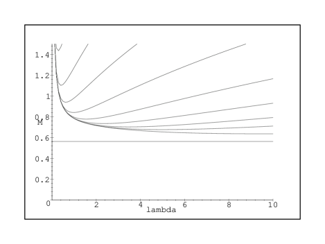
Figure 3: The mass gap over $2\lambda^{1/2}$ vs. $\lambda$ for orders $K=1,2,..,10$ on a lattice of size $N=10$ .

CHIRAL ORDER PARAMETER

An interesting quantity to compute is the vacuum expectation of the chiral condensate per-lattice-site $<\bar{\chi}\chi>$, defined as

$$\bar{\chi}\chi=\frac{1}{2N_{s}}\sum_{x}(-1)^{x}[\hat{\chi}^{\dagger}(\mbox{\bf x}),\hat{\chi}(\mbox{\bf x})],$$ (11)

where $N_{s}$ is the number of lattice sites. The corresponding operator is realized in the P-representation and thus we get for the chiral condensate:

$$\bar{\chi}\chi|P>=(\frac{1}{2}-\frac{2{\cal N}_{P}}{N_{s}})|P>,$$ (12)

where ${\cal N}_{P}$ is the number of connected paths in $P$. To compute $<\bar{\chi}\chi>$ the $\hat{W}$ Hamiltonian is modifyed as

$$\hat{W}^{\prime}=\hat{W}+\frac{\alpha}{2}\sum_{x}(-1)^{x}[\hat{\chi}^{\dagger}(\mbox{\bf x}),\hat{\chi}(\mbox{\bf x})],$$ (13)

where $\alpha$ is an arbitrary parameter. Thus, $<\bar{\chi}\chi>$ is obtained in the standard way as

$$<\bar{\chi}\chi>=\frac{\partial\omega^{\prime}}{\partial\alpha}|_{\alpha=0}.$$ (14)

The massless continuum Schwinger model undergoes a breaking of chiral symmetry with

$$<\bar{\psi}\psi>/e=\frac{e^{\gamma}}{2\pi^{3/2}}=0.15995,$$ (15)

where $\gamma$ is the Euler constant. This non-zero value of the chiral condensate is one of the main efects of the axial anomaly.

In FIG. 4 we report the value of the chiral condensate per-lattice-site for lattice sizes ranging from $N=2$ to $N=10$. FIG. 5 shows this chiral order parameter for different lattice sizes up to order $K=N-2$ for each size.

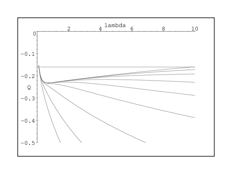
Figure 4: The chiral condensate per-lattice-site times $\lambda^{1/2}$ vs. $\lambda$ for orders $K=1,2,\ldots,10$ on a lattice of size $N=10$ .

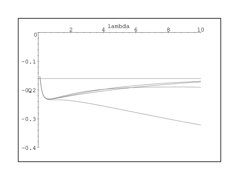
Figure 5: The chiral condensate per-lattice-site times $\lambda^{1/2}$ vs. $\lambda$ on lattices of size $N=4,6,8,10$ for order $K=N-2$ respectively.

Notice that the results in the weak coupling region converge to the corresponding continuum value (15) as long as $N$ increases while for a fixed $N$ the value improves with the order $K$ till the value $K=N-2$ is reached.

4 Conclusions and Final Remarks

Our general proposal is to to show that the P-representation is a valuable and alternative computational tool for gauge theories with dynamical fermions. In particular, in this work, we wanted to test the Hamiltonian approach on finite lattices. With tis aim, we chose the simplest model: (1+1) QED. This also enables us to compare with the corresponding numerical simulations [10] using the Lagrangian counterpart of the P-representation or the socalled worldsheet formulation [11]. This comparison shows that , for this case of one spatial dimension, the Hamiltonian method is less time consuming.

The results are very good and confirm the belief of Hamer et al [6] in obtaining with considerable accuracy the observables working on lattices of moderate size. Consequently, this procedure is appealing because one can run all the needed computations in small machines obtaining quite fair results.

Finally, we would like to stress (once more) that our aim was not to present another solution to the Schwinger model, but, to test an alternative general approach to tackle dynamical fermions.

Acknowledgements

References

- [1] H. Fort and R.Gambini, Phys.Rev. D44 (1991) 1257.
- [2] J.M. Aroca and H. Fort, Phys.Lett.B317 (1993) 604.
- [3] J.M. Aroca and H. Fort, Phys.Lett.B332 (1994) 153.
- [4] S. Coleman, R. Jackiw and L. Susskind, Ann. of Phys. 93 (1975) 267; S. Coleman, Ann. of Phys. 101 (1976) 239.
- [5] D.P. Crewther and C.J. Hamer, Nucl. Phys. B170 (1980) 353.
- [6] C.J. Hamer, Z. Weihong and J. Oitmaa, Phys.Rev. D56 (1997) 55.
- [7] L. Susskind, Phys.Rev. D16 (1977) 3031; Banks T., D.R.T. Jones, J. Kogut, S. Raby, P.N. Scharbach, D.K. Sinclair and L. Susskind, Phys.Rev. D15 (1977) 1111.
- [8] J. Schwinger, Phys. Rev. 128 (1962) 2425.
- [9] T. Banks, L. Susskind and J. Kogut, Phys.Rev. D13 (1976) 1043.
- [10] H. Fort, The Worldsheet Formulation as an Alternative Method for Simulating Dynamical Fermions hep-lat/9710082 October, 1997.
- [11] J.M. Aroca, H. Fort and R. Gambini, hep-lat/9607050.