On the SU(2)-Higgs Phase Transition

Abstract

The properties of the Confinement-Higgs phase transition in the SU(2)-Higgs model with fixed modulus are investigated. We show that the system exhibits a transient behavior up to L=24 along which, the order of the phase transition cannot be discerned. To get stronger conclusions about this point, without going to prohibitive large lattice sizes, we have introduced a second (next-to-nearest neighbors) gauge-Higgs coupling ($\kappa_{2}$). On this extended parameter space we find a line of phase transitions which become increasely weaker as $\kappa_{2}\rightarrow 0$. The results point to a first order character for the transition with the standard action ($\kappa_{2}=0$).

Departamento de Física Teórica, Facultad de Ciencias,
Universidad de Zaragoza, 50009 Zaragoza, Spain
e-mail: isabel@sol.unizar.es

1 Introduction

The generation of mass in the electroweak sector of the Standard Model (SM) [1] relies on the Higgs mechanism. Because of this fact large amount of work has been spent, both, perturbative and non-perturbatively in order to understand the continuum limit of gauge-Higgs models. Underlying is the very question: Does a non-trivial QFT exists in the limit of infinite cut-off ? (see [2] for a review).

On the one hand, it is almost rigorously proved [3, 4] that the pure scalar sector, namely the $\lambda\Phi^{4}$ model, leads to a trivial theory when the cut-off is removed. Of course this is an academic model, and the question is if the coupled gauge-scalar model could produce a non-trivial theory in the continuum.

Perturbatively, the answer seems to be negative, only theories asymptotically free in all the couplings can be constructed [5]. But realistic theories have at least one coupling which is not asymptotically free. A quite accepted scenario describes the SM as an effective theory, with a finite cut-off above which the theory is no longer valid. Within this approach an upper-bound for the Higgs mass can be calculated (see [6] for a review).

However, the non-perturbative sector of the SM is not yet completely understood. The strong self-coupling allowed for the Higgs field, renders perturbation theory useless, and one is forced to use non-perturbative methods to get insight into the properties of the model in this region of couplings.

The Higgs sector of the SM can be approximated by the SU(2)$\otimes$U(1) Higgs model. This approximation is expected to behave reasonably well for the Yukawa couplings between the fermions and the Higgs field, excepting the coupling of the $top$ quark, are small. Also, since the U(1) and the SU(2) gauge couplings are related through the Weinberg angle by $g_{\mathrm{U}(1)}\approx 0.27g_{\mathrm{SU}(2)}$, we can start with the SU(2)-Higgs model, neglecting the U(1) degree of freedom, as a first approximation to describe the electroweak interaction.

In particular, we shall be interested in the limit in which the modulus of the Higgs field is frozen. In the usual notation it correspond to the limit $\lambda=\infty$, being $\lambda$ the parameter controlling the radial degree of freedom of the Higgs field. The phase diagram for this model is well known [7, 8, 9]. A phase transition (PT) line separates a region where the scalar particles are confined in bounded states (confined phase), from another region where the symmetry SU(2)$\otimes$SU(2) is spontaneously broken, and the spectrum consists of the W’s gauge bosons and the Higgs particle (Higgs phase). In this sense SU(2)-Higgs is similar to QCD: there is a phase in which gauge color fields form glueballs and quarks are confined into hadrons, and another phase characterized by the onset of the Higgs mechanism.

The PT line ends at some finite point of the parameter space being both regions analytically connected. So, strictly speaking, we should talk about a single phase, the Confined-Higgs phase (see Figure 1).

Figure 1: Schematic representation of the phase diagram of the SU(2)-Higgs model with frozen modulus ($\lambda=\infty$).

In the scaling region, this model has been extensively studied for small [10] and intermediate [10, 11, 12] values of $\lambda$, where the transition is distinctly first order. The PT weakens when increasing $\lambda$. In the limit $\lambda=\infty$ it is generally believed that the transition is still first order, though extremely weak. However, in our opinion, a higher statistic study in the limit $\lambda=\infty$ is still lacking since the results up to date are not conclusive, as we shall demonstrate. To shed some light on this problem we have studied the model in an extended parameter space too. However, our motivation is not only performing such a large statistics study, but also we want to extract general properties of weak first order phase transitions in coupled gauge-Higgs systems. With this purpose, we have added an extra positive gauge-Higgs coupling between next-to-nearest neighbors to the standard action. We shall use it as a parameter to study the weakening of the PT when this extra coupling is tuned to zero.

In the next section we describe the model, and summarize previous results. In section 3 the numerical method and analysis techniques are detailed. Section 4 contains the results. Finally, the last section is devoted to conclusions.

2 The Model

The SU(2) lattice gauge model coupled to an scalar field, in the fundamental representation of the gauge field can be described by the action

$$S_{\lambda} =\displaystyle\beta\sum_{p}[1-\frac{1}{2}{\mathrm{Tr}}U_{p}]-\frac{1}{2}\kappa_{1}\sum_{x,\mu}{\mathrm{Tr}}\Phi^{\dagger}(x)U_{\mu}(x)\Phi(x+\mu)+$$ (1)

$$\displaystyle+\lambda\sum_{x}[\Phi^{\dagger}(x)\Phi(x)-1]^{2}+\sum_{x}\Phi^{\dagger}(x)\Phi(x)$$

Where U${}_{\mu}(x)$ represents the link variables, and $U_{p}$ are their products along all the positive oriented plaquettes of a four-dimensional lattice of side L.

The scalar field at the site $x$ is denoted by $\Phi(x)$, being $\lambda$ the parameter controlling its radial mode. In the limit ($\lambda=\infty$, $\beta=\infty$) the model becomes a pure O(4)-symmetric scalar model.

As we pointed out in the previous section, the PT line ends at some finite value of the parameters ($\beta$, $\kappa_{1})$ The endpoint moves towards larger $\beta$ values as $\lambda$ increases. For $\lambda\geq 0.1$ the endpoint crosses to the $\beta>0$ region, and in the limit $\lambda=\infty$ the phase transition ends at ($\kappa_{1}\approx 0.6$, $\beta\approx 1.6$) [10]. It is commonly believed that the transition at this point is second order with classical critical exponents [13], however a careful numerical study would be necessary.

In the scaling region, and for finite $\lambda$, the phase transition turns out to be first order. Also, the transition becomes weaker as $\beta$ or $\lambda$ increases. In particular in the limit $\beta=\infty$ (spin model) the transition is second order with classical critical exponents [14].

In the limit $\lambda=\infty$ the situation is less transparent, and it is not clear whether the transition is weak first order or higher order.

The study of the model with the parameter $\lambda=\infty$ is equivalent to fixing the modulus of the Higgs field, $\Phi^{\dagger}\cdot\Phi=1$. In the pioneer work, [15], the PT was considered first order for finite $\lambda$ and second order for $\lambda=\infty$. Later, larger statistics, and the hypothesis of a universal behavior of the PT for all values of $\lambda$, seem to point to a first order character of the PT in the scaling region. Nowadays, though it is generally believed that the transition is still first order in this limit, the numerical proofs [16, 11] on which rely these statements are not conclusive, as the authors safely conclude, because the statistic and lattice sizes are not enough for excluding the possibility of a higher order phase transition in the edge $\lambda=\infty$.

The model with fixed modulus is described by the action

$$S_{\infty}=\beta\sum_{p}[1-\frac{1}{2}{\mathrm{T}r}U_{p}]-\frac{1}{2}\kappa_{1}\sum_{x,\mu}{\mathrm{T}r}\Phi^{\dagger}(x)U_{\mu}(x)\Phi(x+\mu)$$ (2)

As we shall show below, we have simulated this model up to lattices L=24, and the result is still compatible with a second or higher order PT, however, we have no indications of asymptoticity in the behavior of the observables, and the results are compatible with a very weak first order PT too. This means that larger lattices are needed to overcome these transient effects, but the added difficulty here is that such lattices would suffer of termalization problems, and severe autocorrelation times. Altogether makes this approach too CPU expensive for nowadays computers.

In order to get a more conclusive answer without going to prohibitive large lattice sizes, we have studied the model in an extended parameter space. For this purpose we have introduced a second coupling between the gauge and the scalar field connecting next-to-nearest neighbors on the lattice, in such a way that the new action reads

$$S=S_{\infty}-\frac{1}{4}\kappa_{2}\sum_{x,\mu<\nu}Tr\Phi^{\dagger}(x)[U_{\mu}(x)U_{\nu}(x+\mu)+U_{\nu}(x)U_{\mu}(x+\nu)]\Phi(x+\mu+\nu)$$ (3)

Within this parameter space we expect to get a global vision on what the properties of the PT are, and also, to give a stronger conclusion about the order. In the region of $\kappa_{2}$ positive, (competing interaction effects appear if $\kappa_{2}<0$) this extended model is expected to belong to the same universality class than the standard one ($\kappa_{2}$ = 0) since both models posses the same symmetries. The effect of the new coupling $\kappa_{2}>0$ is to reinforce the transition but should not change the order if the system has not tricritical points. An example of such behavior appears in the O(4)-symmetric $\sigma$ model with second neighbors coupling. This model presents a ($\kappa_{1}^{c},\kappa_{2}^{c}$) line of phase transitions which is second order, since the model with $\kappa_{2}=0$ shows a second order PT too [17].

The action (3) has the following symmetries:

• $\kappa_{1}=\kappa_{2}=0$.

  $$\beta \rightarrow -\beta$$

  $$U_{\mu}(x) \displaystyle\rightarrow (-1)^{\sum_{\rho\neq\mu}x_{\rho}}U_{\mu}(x)$$ (4)

• $\kappa_{1}\rightarrow-\kappa_{1}$, $\Phi(x)$ fixed

  $$U_{\mu}(x)\rightarrow-U_{\mu}(x)$$ (5)

• $\kappa_{1}\rightarrow-\kappa_{1}$, $U_{\mu}(x)$ fixed

  $$\Phi(x)\rightarrow\displaystyle(-1)^{\sum_{\mu=0}^{d-1}x_{\mu}}\Phi(x)$$ (6)

The action is not symmetric under the change $\kappa_{2}\rightarrow-\kappa_{2}$. The existence of couplings $\kappa_{1}$ and $\kappa_{2}$ with opposite signs would make frustration to appear, and very different vacua are possible [17]. This region present problems when one tries to implement reflection positivity, however, the possibility of defining a continuum limit at this region is not discarded a priori [18]. In this work we are interested in the regions free of frustration effects. Taking into account the symmetry properties of the action, the phase diagram in the region $\kappa_{2}>$ 0 will be symmetric with respect to the axis $\kappa_{1}$ = 0, and hence, we can restrict the study to the quadrant $\kappa_{1}>$ 0.

We define the normalized energy associated to the plaquette term

$$E_{0}=\frac{1}{N_{l_{0}}}\sum_{p}(1-\frac{1}{2}{\mathrm{Tr}}U_{p})$$ (7)

and also the energies associated to the links

$$E_{1}=\frac{1}{N_{l_{1}}}\sum_{x,\mu}\frac{1}{2}{\mathrm{Tr}}\Phi^{\dagger}(x)U_{\mu}(x)\Phi(x+\mu)$$ (8)

$$E_{2}=\frac{1}{N_{l_{2}}}\sum_{x,\mu<\nu}\frac{1}{4}{\mathrm{Tr}}\Phi^{\dagger}(x)[U_{\mu}(x)U_{\nu}(x+\mu)+U_{\nu}(x)U_{\mu}(x+\nu)]\Phi(x+\mu+\nu)$$ (9)

where $N_{l_{0}}$ = 6V, $N_{l_{2}}$ = 12V and $N_{l_{1}}$ = 4V.

With these definitions $E_{0}\rightarrow 0$ when $\beta\rightarrow\infty$ and $E_{i}\rightarrow 1$ when $\kappa_{i}\rightarrow\infty$.

On the three-dimensional ($\beta$, $\kappa_{1}$, $\kappa_{2}$) parameter space we consider the plane $\beta=2.3$. On this plane there is a PT line ($\kappa_{1}^{c},\kappa_{2}^{c}$). We expect to learn on the properties of this PT on the region ($\kappa_{1}^{c}\neq 0,\kappa_{2}^{c}\neq 0$), where the signals are clearer, with regards to applying what we learn to the $\emph{s}tandard$ case $\kappa_{2}=0$.

To monitorize the strength of the phase transition, we measure the existence of latent heat, and the behavior of the specific heat. As we shall see, for $\kappa_{1}=0$ the transition is first order, with a clearly measurable latent heat. We will see how this transition weakens along the PT line for increasing values of $\kappa_{1}$.

Figure 2: Phase diagram obtained from the MC simulation.

3 Numerical study

Figure 3: Normalized energy distribution for L=12, $\lambda=\infty$, $\kappa_{1}$=0.395, $\beta$=2.3 from [16] (dotted line), compared with the distribution we obtain at the same couplings (solid line) in $L$=12 too, when statistics is increased by one order of magnitude.

We have simulated the model in a $L^{4}$ lattice with periodic boundary conditions. For the update we have employed a combination of heat-bath and over-relaxation algorithms (ten over-relax sweeps followed by a heat-bath sweep). For the simulation we used the RTNN machine, consisting of a network of 32 PentiumPro 200MHz. processor. The total CPU time employed has been the equivalent of 3 years of PentiumPro.

Monte Carlo methods provide information about the thermodynamic quantities at a particular value of the couplings. We have used the Spectral Density Method (SDM) [19] to extract information on the values of the observables in a finite region around the simulation point. In particular it is useful to have a precise location of the coupling where some observables have a maximum, as well as an accurate measure of the value of that maximum.

From the Monte Carlo simulation at some coupling $\kappa$, we got the histogram $H(E)$ which is an approximation to the density of states. Using the SDM approximation the probability of finding the system with an energy E at a different coupling $\kappa^{\prime}$ can be written as:

$$P_{\kappa^{\prime}}(E)\propto H(E)e^{(\kappa^{\prime}-\kappa)VE}$$ (10)

The region of validity of the SDM approximation is $\Delta\kappa\sim 1/(V\sigma)$, being $\sigma$ the width of the distribution $H(E)$. Although $\sigma$ gets the maximum values in the critical region, the approximation has been very useful, specially for tuning the couplings where to measure.

Concerning the lattice sizes, we have used lattices ranging from $L$=6 to $L$=24. For the small lattices ($L$=6, 8 and 12) we have done 4$\times$10${}^{5}\tau$ iterations, being $\tau$ the largest autocorrelation time for the energy, which ranges from $\tau\approx 10$ in $L$=8 to $\tau\approx 35$ in $L$=24. For the largest lattices, $L$=20 and 24, we run up to 10${}^{5}\tau$ MC iterations.

The statistical errors are computed with the jackknife method.

4 Results

We shall make the discussion with the first-neighbors link energy, E₁, but as far as the critical behavior is concerned, we could carry out the analysis with any of the energies. We remark that an appropriate linear combination of E₁, E₂ and E₀ could give slightly more accurate results [20].

We have considered fixed values of $\kappa_{1}$ (0, 0.02, 0.1, 0.2 and 0.3) and sought the $\kappa_{2}$ critical for every line, $\kappa_{2}^{c}(\kappa_{1})$. We have also studied the case $\kappa_{2}$= 0 varying $\kappa_{1}$ which corresponds to the usual SU(2)-Higgs model.

The SDM has been used to locate the apparent critical point, defined through the specific heat behavior. From the specific heat matrix

$$C_{v}^{i,j}(L)=\frac{\partial E_{i}}{\partial\kappa_{j}}$$ (11)

we obtain the best signal for C${}_{v}^{1,2}(L)$, which can be calculated as (we shall omit the superscript from now on)

$$C_{v}(L)=4L^{d}(\langle E_{1}E_{2}\rangle-\langle E_{1}\rangle\langle E_{2}\rangle)$$ (12)

In a first order phase transition, C${}_{v}^{\mathrm{max}}(L)$ behaves, asymptotically, proportional to the volume, $L^{d}$. If the PT is second order, the dominant behavior for C${}_{v}(L)^{\mathrm{max}}$ is $L^{\alpha/\nu}$ which diverges too provided that $\alpha>$ 0. At the upper critical dimension $\alpha$ = 0, and one has to go further the leading order, appearing logarithmic divergences [21].

As a consequence of this divergent behavior, in a finite lattice C${}_{v}(L)$ shows a peak at some value of the coupling which will be taken as apparent critical point, $\kappa_{2}^{\ast}(L)$.

In Figure 2 we plot the critical line ($\kappa_{1}^{c},\kappa_{2}^{c}$). This line is obtained by extrapolation to the thermodynamic limit according to $\kappa_{2}^{c}(\infty)=\kappa_{2}^{\ast}(L)-AL^{-d}$. We point out that this extrapolation is valid only in first order phase transitions. If the PT is second order the power in $L$ is ($-1/\nu$).

In continuous PT scale invariance holds, and the thermodynamic magnitudes, such as the specific heat, or susceptibilities do scale. However if the transition is first order the correlation length remains finite and hence there is not scaling properties, and no critical exponents can be defined.

Nevertheless in a first order PT we can ask how large is the lattice we need in order to observe the asymptotic behavior of C_v. In particular, with abuse of language one can measure a $\emph{p}seudo$ $\alpha/\nu$ exponent to get insight on the nature of the PT: the larger is the lattice we need to measure $\nu=1/d$, the weaker the PT is. Following this, first order PT can be classified according to their degree of weakness.

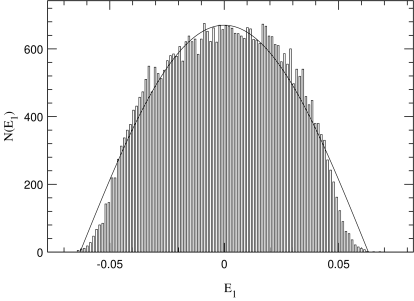
Figure 4: E₁ distribution on the axis $\kappa_{1}=0$ on a L=8 lattice. at ($\kappa_{2}=0.15,\beta=2.3$). The cosine fit is very accurate in spite of the finite $\beta$ value, in this region of parameters the pure gauge term couples slightly both sub-lattices.

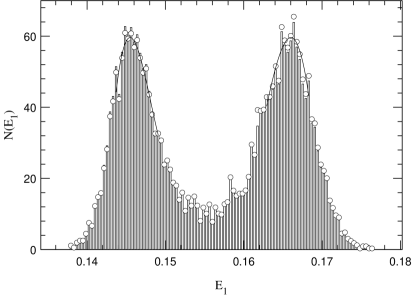
Figure 5: Normalized distribution of E₁ at ($\kappa_{1}=0.2$, $\kappa_{2}=0.10036$) in a L=16 lattice. The cubic fit at the maxima to get $\Delta E$ is superimposed.

Figure 6: MC evolution of E₁ at ($\kappa_{1}=0.2,\kappa_{2}^{\ast}(L)$) for $L$=8 (lower part), $L$=12 (middle) and $L$=16 (upper part).

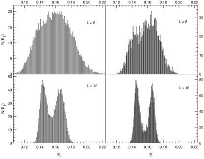
Figure 7: Normalized distribution of E₁ at ($\kappa_{1}=0.2,\kappa_{2}^{\ast}(L)$) for L=6, 8, 12 and 16.

However, the so called weak first-order PT appear often in literature (see [22, 23] and references there in) as PT characterized by a transient behavior with a non-measurable latent heat. Let be $\xi_{c}$ the correlation length of the system at the critical point in the thermodynamic limit. In a finite lattice of size $L$, the first order behavior will be evidenced if $L\geq\xi_{c}$. For lattice sizes much smaller than $\xi_{c}$ the system will behave like in a second-order PT, since the correlation length is effectively infinite. As an example, in Figure 3 we plot the energy distribution in a L=12 lattice at ($\beta=2.3,\kappa_{1}=0.395$) obtained in [16], compared with the one we obtain at the same couplings and in the same L, when the statistics increases by one order of magnitude. We observe that the order of the PT can not be discerned at this volume, even when the statistics is enough. Termalization effects can also contribute to mistake the histogram structure.

The entire line ($\kappa_{1}^{c},\kappa_{2}^{c}$) is first order, but the weak character increases as $\kappa_{2}\rightarrow 0$. We will make a quantitative description of the weakening phenomenon by studying the specific heat, and the latent heat.

But before going on, we shall make a remark concerning the behavior on $\kappa_{1}=0$. As we pointed out, the system is symmetric under the change $\kappa_{1}\rightarrow-\kappa_{1}$. The transformation (6) maps the positive $\kappa_{1}$ semi-plane with energy E₁, onto the negative $\kappa_{1}$ semi-plane with energy -E₁. The transition across this axis is first order because the energy is discontinuous. In the limit $\beta\rightarrow\infty$, and in $\kappa_{1}=0$, the system decouples in two independent sublattices, each one constituted by the first neighbors of the other. The first neighbors energy for this system is proportional to $\cos\theta$, being $\theta$ the angle between the symmetry breaking direction of the scalar field in both sub-lattices. In Figure 4 we plot the E₁ distribution for L=8 at $(\kappa_{1}=0,\kappa_{2}=0.15)$ and $\beta=2.3$. We see that the agreement with a cosine distribution is quite good in spite of the finite $\beta$ value.

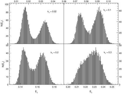
Figure 8: Normalized distributions of E₁ for $\kappa_{1}$ = 0.02, 0.1, 0.2 and 0.3 at $\kappa_{2}^{\ast}(12)$.

Figure 9: Normalized distribution of E₁ at $\kappa_{1}$ = 0.3 for L=12,16 and 20

4.1 Latent Heat

Along the apparent critical line we have done simulations for different lattice sizes and stored the plaquette and links energies to construct the histograms for the energy distributions. In a first-order phase transition the energy has a discontinuity which manifest in the appearance of latent heat, $\Delta E$. This quantity is not well defined in a finite lattice, so we measure the distance between the two maximum of the energy distribution, and extrapolate to the thermodynamic limit. The drawback of this approximation is that the maxima of the energy distribution are difficult to discern, since this function at the apparent critical point is very noisy We have used a cubic spline at the maxima in order to get a more reliable estimation (Figure 5).

In Figure 6 we show the MC evolution of E₁ for $L$=8, 12 and 16 at $\kappa_{1}=0.2$. In $L$=8 the latent heat is not clearly measurable. We observe in the MC evolution how the two-state signal becomes cleaner as the lattice size increases (see Figure 7).

In Figure 7 we plot the distribution of E₁ at $\kappa_{1}=0.2$ at the apparent critical point $\kappa_{2}^{\ast}(L)$ for $L$=6, 8, 12 and 16. A remarkable stability of $\Delta E_{1}$ with the volume is observed. This is a common feature for all values of $\kappa_{1}$.

As we have already pointed out, the transition weakens when increasing $\kappa_{1}$ and larger lattices are needed in order to observe a measurable latent heat. We give a quantitative description of this fact in Figure 8, where the distribution of $E_{1}$ for several values of ($\kappa_{1},\kappa_{2}^{\ast}(12)$) is displayed. The two-state signal is no longer measurable in $L$=12 at $\kappa_{1}=0.3$. The first evidences of two-states appear in $L$=20 (see Figure 9). but from its energy distribution we can only give an approximate value for $\Delta E_{1}(L=20)$ since the two-peaks appear too close to each other.

In Figure 10 we plot $\Delta E_{1}(L)$ and $\Delta E_{2}(L)$ as a function of 1/L⁴, in order to get $\Delta E_{i}$ in the thermodynamic limit with a linear fit. Finally we quote these values in Table 1, together with the change in the action (3) between the two phases.

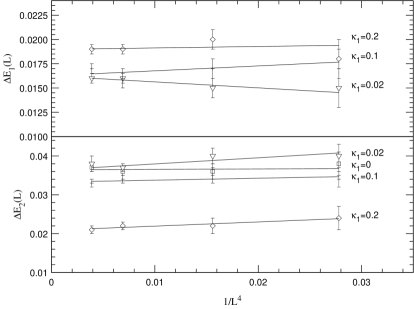
Figure 10: $\Delta E_{1}$ (upper plane) and $\Delta E_{2}$ (lower plane) as a function of 1/L⁴. The two-peak structure is not clearly observed in L=6 at any $\kappa_{1}$ value. The values quoted for this lattice size are upper bounds.

Figure 11: Normalized distribution of E₁ at $\kappa_{2}$=0, in $L$=16, 20 and 24 at the peak of the specific heat

coupling	$\Delta E_{1}(\infty)$	$\Delta E_{2}(\infty)$	$\Delta S$
$\kappa_{1}$ = 0	-	0.0366(8)	0.0134(12)
$\kappa_{1}$ = 0.02	0.0162(6)	0.0347(5)	0.0137(13)
$\kappa_{1}$ = 0.1	0.0162(7)	0.0345(9)	0.0094(10)
$\kappa_{1}$ = 0.2	0.0179(7)	0.0201(8)	0.0078(12)
$\kappa_{1}$ = 0.3	$\approx$0.006	$\approx$ 0.012	$\approx$ 0.0026

Table 1: $\Delta E(\infty)$ for E₁ and E₂, and variation of the action.

From the energy distributions at $\kappa_{2}=0$, see Figure 11 we have no direct evidences of the existence of latent heat. However, on the larger lattices one can observe non-gaussianities in the energy distributions. Such asymmetries could precede the onset of clear two-peak structures in larger lattices, however this is just a guess. We conclude that no information concerning the order of the PT can be obtained from the energy distributions up to $L$=24.

4.2 Specific Heat

We have done MC simulations at the points predicted by SDM, ($\kappa_{1},\kappa_{2}^{\ast}(L)$), in order to measure accurately the peak of $C_{v}(L)$.

As an example we show in Figure 12 the value of $C_{v}(L)$ around its maximum for various lattice sizes at $\kappa_{1}$ = 0.2 (upper plane) and at $\kappa_{1}$ = 0.3 (lower plane). We observe that the maximum of the specific heat grows slower when increasing $\kappa_{1}$, indicating a weakening in the PT.

Figure 12: C${}_{v}^{\mathrm{max}}(L)$ at $\kappa_{1}=0.2$ (lower plane), at $\kappa_{1}=0.3$ (middle) and at $\kappa_{2}=0$ (upper plane). The dotted line is the SDM extrapolation.

In Figure 13 we draw C${}_{v}^{\mathrm{max}}(L)$ relative to C${}_{v}^{\mathrm{max}}(6)$ as a function of the lattice size. The values have been normalized to C${}_{v}^{\mathrm{max}}(8)$/C${}_{v}^{\mathrm{max}}(6)$ in order to compare distinctly the behaviors for different $\kappa_{1}$. The slope of the segment joining the values of C${}_{v}^{\mathrm{max}}$ in consecutive lattices gives the $pseudo$ $\alpha/\nu$ exponent. We observe that such slope is approximately 4 at $\kappa_{1}$ = 0.02, 0.1 and 0.2 for all the volumes we compare. However the transition at $\kappa_{1}$ = 0.3 evidences much more weakness. We do not have evidences of asymptoticity in C${}_{v}^{\mathrm{max}}$ till L=20, as could be expected from the energy distributions (Figure 9). The slope of the segment joining C${}_{v}^{\mathrm{max}}(16)$ with C${}_{v}^{\mathrm{max}}(20)$ is 3.05(12) which is almost the asymptotic value expected for a first order PT.

As expected, only if the two-peak structure is observed in the energy distributions and $\Delta E$ is stable, the maximum of the specific heat will grow up like the volume, $L^{d}$.

At $\kappa_{2}$ = 0 we are within the transient region even for L=24. We remark that in this case C_v is defined by the element C^1,1 of the specific heat matrix (11) since this is the most natural choice at this point, and also is the best signal we measure. As we observe in Figure 13, at $\kappa_{2}$ = 0 C${}_{v}^{\mathrm{max}}(L)$ seems to tend to a constant value as V$\rightarrow\infty$ up to $L$=20. From our previous discussions we should conclude that either the correlation length at the transition point $\xi_{c}$ is much larger than the lattice size up to L=20, or the transition is second order with $\alpha=0$ in the thermodynamic limit. However, in $L$ = 24 things are changing, C${}_{v}^{\mathrm{m}ax}(L=24)$ starts to run away of this quasi-plateau, and the $pseudo$ $\alpha/\nu$ exponent grows again. As can be observed in Figure 13, at $\kappa_{1}$ = 0.3 the $pseudo$ $\alpha/\nu$ exponent decreases for the segment $L$ = 12-16, with respect to the value in the segment $L$ = 8-12. The lattice $L$ = 20 is enough to overcome the transient region, but the behavior is qualitatively the same that in $\kappa_{2}$ = 0, though the transition is stronger.

We believe that this behavior is general for weak first order transitions in four dimensions. There exists a transient region in which the correlation length is effectively infinite compared with the lattice size, and the system behaves like suffering a second order PT with thermal index $\alpha\approx 0$ in the thermodynamic limit.

Figure 13: C${}_{v}^{\mathrm{max}}$ for the various $\kappa_{1}$ values and $\kappa_{2}=0$. We have normalized the values with respect to C${}_{v}^{\mathrm{max}}$(8)/C${}_{v}^{\mathrm{max}}$(6). The slope of the segments is indicated when smaller than 4.

4.3 Binder Cumulant

In order to check the consistency of our results we have also considered the behavior of the Binder cumulant

$$V_{L}=1-\frac{\langle E_{1}^{4}\rangle_{L}}{3\langle E_{1}^{2}\rangle_{L}^{2}}$$ (13)

This quantity behaves differently depending on the order of the PT. If the transition is second order the minimum of the cumulant, $V_{L}^{min}$ approach 2/3 in the thermodynamic limit. However if the transition is first order, $V_{L}^{min}$ tends a value smaller than 2/3 reflecting the non-gaussianity of the energy distribution at the transition point.

In Figure 14 we plot $V_{L}^{\mathrm{min}}$ for several $\kappa_{1}$ values.

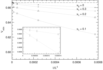
Figure 14: $V_{L}^{min}$ for $\kappa_{1}$ = 0.1, 0.2,0.3 and $\kappa_{2}$ = 0, as a function of 1/L⁴. The dashed line represents the value 2/3.

For those values of $\kappa_{1}$ in which the PT is distinctly first order, the minimum of the Binder cumulant stays safely away from 2/3, as we observe $V_{L}^{min}$ extrapolated to L$\rightarrow\infty$ is 0.65401(4) at $\kappa_{1}$ = 0.1. However, this value reachs 0.66637(5) at $\kappa_{1}$ = 0.3, and 0.66657(8) at $\kappa_{2}=0$. Again we find a tight difference between a very weak first order PT and a continuous one.

For the sake of discussing quantitatively the order of magnitude of the latent heat in the limit $\kappa_{2}=0$, from the energy distributions we find that at $\kappa_{2}=0$ one can approximately locate one the peaks of the energy at E${}_{a}\approx$ 0.273. The other should be at certain E_b = E${}_{a}-\Delta$, being $\Delta$ the latent heat.

In the thermodynamic limit the energy distributions are two delta functions situated at E_a and E_b, then

$$V_{\infty}^{min}=1-\frac{2(E_{a}^{4}+E_{b}^{4})}{3(E_{a}^{2}+E_{b}^{2})^{2}}$$ (14)

If we use V${}_{\infty}^{min}$ = 0.66657 and E_a in (14) the value we got for the latent heat is $\Delta\approx 0.006$ which is of the same order as the one expected from the histograms.

5 Conclusions

The order of the Confinement-Higgs phase transition in the SU(2)-Higgs model with fixed modulus is a highly non trivial issue. We have used an extended parameter space, in order to get a global vision on the problem. On this extended parameter space we have found a line of first order phase transitions which get weaker as $\kappa_{2}\rightarrow$ 0. We have also observed that, because of the computer resources needed, it is too ambitious trying to measure two-peak energy distributions in the limit $\kappa_{2}$ = 0. However, on this point, we can get conclusions from the behavior of the specific heat.

As we have discussed along the paper, a fake second order PT seems to exists for a range of $L$ in very weak first order phase transitions. We have applied Finite Size Scaling properties along this transient region to compute a $pseudo$ $\alpha/\nu$ critical index. We want to be extremely careful at this point, this computation is completely meaningless when the transition is first order, since Scaling does not hold, but it can be used as a technical tool to catalogue the PT when there is no direct evidences, as in this case. Using the relation $\alpha=2-\nu d$, we got $\nu$ varying in the interval (0.36, 0.41) in the range $L=8,\dots,20$. Calculated from $L$=20 and $L$=24, $\nu\approx 0.35$. We expect this behavior to be transitory, and when going to larger lattices sizes, if the transition is second order, $\nu$ should reach its mean field value $\nu=1/2$. If the transition is first order this value should go to 1/d, indicating that the specific heat maximum grows like the volume $L^{d}$. We believe that this is the case, since the $pseudo$ $\nu$ exponent in $L$=24, instead of approaching 1/2, starts to decrease. An example of weak first order PT showing a similar behavior is described in [25].

In what concerning the motivation of introducing a second coupling, we pointed out that $\kappa_{2}$ should not change the order of the PT because do not change the symmetry properties. This argument is heuristic, but the phase diagram we found supports this assertion. As far as the order of the PT is concerned, we think that this approach can be useful when dealing with PT of questionable order in the sense that it is not clear whether the transition is weakly first order or higher order. The hope is that it could be applied to other more controversial models.

I thank A. Tarancón and L.A. Fernández for comments and advice.

References

- [1] S. Weinberg. Phys. Rev. Lett. 19, p 1264 (1967)
- [2] D. E. Callaway, Phys. Rep. 165, p 5 (1988)
- [3] M. Aizenman. Phys. Rev. Lett. 97, p 1 (1981)
- [4] J. Frolich. Nuc. Phys. B200 [FS4], p 281 (1982)
- [5] A. Hasenfratz and P. Hasenfratz. Phys. Rev. D34, p 3160 (1986)
- [6] A. Hasenfratz in Quantum Fields on the Computer World Scientific Publishing, Singapore / Editor M. Creutz (1992)
- [7] J. M. Drouffe and J. B. Zuber. Phys. Rep. 102, p 1 (1983)
- [8] E. Fradkind and E. Shenker. Phys. Rev. D19, p 3682 (1979)
- [9] M. Creutz, L. Jacobs and C. Rebbi. Phys. Rep. 95, p 201 (1983)
- [10] J. Jersak, C.B. Lang, T. Neuhaus and G. Vones. Phys. Rev. D32, p 2761(1985)
- [11] W. Langguth, I. Montvay and P. Weisz. Nuc. Phys. B277, p 11(1986)
- [12] W. Bock, H. G. Evertz, J. Jersak, D.P. Landau, T. Neuhaus and J. L. Xu. Phys. Rev. D41, p 2573(1990)
- [13] D.J.E. Callaway and R. Petronzio Nuc. Phys. B267, p 253 (1986)
- [14] C. Itzykson and J.M. Drouffe. Statistical Field Theory, Vol. 1. Cambridge University Press, / Cambridge, England (1989)
- [15] C.B. Lang, C. Rebbi and M.A. Virasoro. Phys. Lett. B104, p 294(1981)
- [16] W. Langguth and I. Montvay Phys. Lett. B165, p 135(1985)
- [17] I. Campos, A. Tarancón and L.A. Fernández. Phys. Rev. D55, p 2965 (1997)
- [18] J. Fingberg and J. Polonyi Nuc. Phys. B486, p 315 (1997)
- [19] A. M. Ferrenberg and R. Swendsen. Phys. Rev. Lett. 61, p 2635(1988)
- [20] RTN collaboration (J.L. Alonso et al.) Nuc. Phys. B405, p 574 (1993)
- [21] E. Brezin, J.C. Le Guillou and J. Zinn-Justin. “Field Theoretical approach to critical phenomena” in Phase Transitions and Critical Phenomena ed. C. Domb and M.S. Green (Academic Press, London) (1976).
- [22] J.J. Ruiz-Lorenzo Ph.D. Thesis U. Complutense de Madrid (1993)
- [23] L.A. Fernández, M.P. Lombardo and J.J. Ruiz-Lorenzo. Phys. Lett. B277, p 485(1992)
- [24] M.S.S. Challa, D.P. Landau and K. Binder. Phys. Rev. B34, p 1841 (1986)
- [25] J.L. Alonso, J.M. Carmona, J. Clemente, L.A. Fernández, D. Iñiguez, A. Tarancón and C.L. Ullod. Phys. Lett. B376, p 148 (1996)