CERN-TH/97-111

LPTHE-ORSAY/97-32

June 1997

A Wilson-Yukawa Model with undoubled chiral fermions in 2D

P. Hernández

Theory Division, CERN

CH-1211 Geneva 23, Switzerland

Ph. Boucaud

LPTHE, Université de Paris XI

91405 Orsay Cedex, France.

We consider the fermion mass spectrum in the strong coupling vortex phase (VXS) of a lattice fermion-scalar model with a global $U(1)_{L}\times U(1)_{R}$, in two dimensions, in the context of a recently proposed two-cutoff lattice formulation. The fermion doublers are easily made massive by a strong Wilson-Yukawa coupling, but in contrast with the standard formulation of these models, in which the light fermion spectrum was found to be vector-like, we find massless fermions with chiral quantum numbers at finite lattice spacing. When the global symmetry is gauged, this model is expected to give rise to a lattice chiral gauge theory.

1 Introduction

Wilson-Yukawa models were extensively studied some years ago as a possible lattice formulation of chiral gauge theories [1]. The idea was to decouple the lattice doublers from the light spectrum by introducing the so-called Wilson-Yukawa term, which contains a charged scalar field in a way that it is manifestly gauge invariant under a chiral gauge transformation. With the addition of this “Higgs” particle, it was expected that doublers would decouple, while chiral fermions would remain in the light spectrum. This expectation was based on the numerical finding of a strong Yukawa-coupling regime, both in the symmetric (PMS) and broken (FMS) phases, where the fermion masses are not proportional to the vacuum expectation value of the scalar field, as in the perturbative regime, and doublers can get masses of the order of the cutoff. However, for the same reason, also the light fermions are massive in this phase (although their mass could be tuned to zero by tuning the bare mass). More problematic was the fact that the light fermions were found to have only vector-like couplings to the gauge fields. The physical picture that emerged from these results was that in the strong coupling phase, composites of the light fermions and the scalar particles were formed, generating effective mirror states and rendering the theory vector-like. This situation was found already in the quenched approximation.

It is important to realize that the failure of Wilson-Yukawa models is also very relevant for all those lattice proposals of chiral gauge theories that explicitly break the gauge symmetry. The reason is that, once gauge invariance has been broken for a compact group, the gauge non-invariant theory is exactly equivalent to a gauge-invariant theory with new charged scalar degrees of freedom [2]. The scalar degrees of freedom are nothing more than the pure gauge transformations. The effective action of these scalars differs in general from one proposal to another, but they are coupled as long as gauge invariance is broken in the original formulation and so they must be dealt with. In particular, the simplest formulation of chiral gauge theories, which introduces a standard Wilson term to decouple doublers, breaks gauge invariance and is in one-to-one correspondence to the Wilson-Yukawa models considered in [1]. Equivalently all proposals that break gauge invariance must have a corresponding Wilson-Yukawa picture. It is important to understand to what extent the failures of these models in providing a regularization for chiral gauge theories are circumvented by other proposals.

Recently a new method has been proposed to regulate chiral gauge theories on the lattice [3]. In this approach, the fermions live on a lattice of spacing $f$ and are coupled to gauge link variables that are constructed by an appropriate smooth and gauge-invariant interpolation of gauge configurations [4] that are generated on a coarser lattice of spacing $b$. This construction corresponds to a two-cutoff lattice regulator (TC), where fermion momenta are cut off at a much larger scale $1/f$ than the gauge boson momenta $1/b$. Doublers are decoupled by introducing a naive Wilson term as in the Roma approach [5]. However, since the chirally breaking effects due to the Wilson term are relevant only at scales of the order of the fermion cutoff, gauge boson momenta are not large enough to prove these interactions, in contrast with one-cutoff (OC) formulations. As a result, due to the separation of the cutoff scales, no fine-tuning is necessary to recover an approximate chiral gauge symmetry, as long as the ratio $f/b$ is small enough. In other words, gauge invariance is broken but there is a small parameter, $f/b$, which controls the strength of this breaking. As we will see, there are good arguments to believe that a “small” breaking of gauge invariance does not have a dramatic effect at large distances [6]. The two-cutoff construction is the first proposal that has a control over the strength of this breaking.

In this paper we want to consider the Wilson-Yukawa picture of the TC formulation of [3] and show evidence that in fact a chiral phase exists, in contrast to what was found in OC formulations. In order to address these issues numerically, we have considered the simplest relevant model, which is a $U(1)$ compact theory in two dimensions, in the quenched approximation. The model contains one left-handed fermion coupled to $U(1)$ gauge fields . In order to get rid of doublers, a right-handed fermion is introduced, which only couples through the Wilson term. In the global limit ($g\rightarrow 0$, i.e. only the pure gauge transformations are coupled) the Wilson-Yukawa picture is a scalar-fermion model with an exact global symmetry $U(1)_{L}\times U(1)_{R}$. This model has been previously considered in a standard OC formulation in [8], where it was found that the fermion spectrum was either doubled (in the weak Yukawa phase) or vector-like (in the strong Yukawa phase). We will show that in the TC formulation a truly chiral phase exists.

The paper is organized as follows. In section 2, we review the relation between gauge-non-invariant formulations of chiral gauge theories and models of the Wilson-Yukawa type. In section 3, we present the two-cutoff lattice formulation of the two-dimensional model under study and its equivalent Wilson-Yukawa picture. In section 4, we discuss the expected phases of this model and why a phase with massless chiral fermions should exist. In section 5, we present our numerical results on the fermion spectrum, which support the existence of a chiral phase. In section 6 we briefly discuss the effects of unquenching and conclude in section 7.

2 Wilson-Yukawa picture of $\chi GTh$

As explained in the introduction, all proposals to regulate chiral gauge theories which break the gauge symmetry are equivalent to a model with an exact gauge invariance and additional charged scalars [2]. This is simple to see. Let us consider a lattice action that contains gauge-breaking interactions,

$$S[U,\Psi]=S_{g.i.}[U,\Psi]+\delta S_{n.g.i.}[U,\Psi]$$ (1)

The path integral is

$$Z=\int{\cal D}U_{\mu}\int d\Psi d\bar{\Psi}\;\;e^{-S_{g.i}[U,\Psi]-\delta S_{n.g.i.}[U,\Psi]}.$$ (2)

Since the group is compact we can multiply $Z$ by the volume of the group $\int{\cal D}\Omega$, which is an irrelevant constant factor:

$$Z=\int{\cal D}\Omega\int{\cal D}U_{\mu}\int d\Psi d\bar{\Psi}\;\;e^{S_{g.i}[U,\Psi]+\delta S_{n.g.i.}[U,\Psi]}.$$ (3)

Performing a change of variables, from $U_{\mu}$ to $U^{\Omega}_{\mu}\equiv\Omega(x)U_{\mu}(x)\Omega^{\dagger}(x+\hat{\mu})$ (i.e. the gauge-transformed variables under the lattice gauge transformation $\Omega$), and from $\Psi$ to $\Psi^{\Omega(x)}=\Omega(x)\Psi(x)$ (only for the charged fermions), and using the invariance of the measure and $S_{g.i.}$ under a gauge transformation, we get

$$Z=\int{\cal D}\Omega\int{\cal D}U_{\mu}\int d\Psi d\bar{\Psi}\;\;e^{S_{g.i}[U,\Psi]+\delta S_{n.g.i.}[U^{\Omega},\Psi^{\Omega}]}.$$ (4)

It is easy to see that (4) is gauge-invariant under a new gauge symmetry under which the field $\Omega$ transforms

$$U_{\mu}(x) \rightarrow \Phi(x)U_{\mu}(x)\Phi^{\dagger}(x+\hat{\mu})\;\;\;\;\Omega(x)\rightarrow\Omega(x)\Phi(x)^{\dagger}$$

$$\Psi^{(c)} \rightarrow \Phi(x)\Psi^{(c)}(x)\;\;\;\;\;\;\;\;\Psi^{(n)}\rightarrow\Psi^{(n)}(x),$$ (5)

where $c,n$ are charged and neutral fermion fields respectively. This is because $\Psi^{\Omega}$ and $U_{\mu}^{\Omega}$ are invariant under this transformation. This theory is then a gauge theory with extra charged scalars in a non-linear realization ($\Omega$ is unitary). These scalars are the pure gauge transformations, which couple through the non-invariant terms in the original action. It is clear that in any successful proposal for regulating chiral gauge theories, these scalars must decouple from the light physical spectrum. In the case of a spontaneously broken gauge theory these degrees of freedom remain, since they become the longitudinal gauge bosons. This is however not our objective here, since we aim at regulating a symmetric chiral gauge theory. The interesting case of spontaneous symmetry breaking will be considered elsewhere.

Foester, Nielsen and Ninomiya (FNN) gave in [6] a good argument why a gauge theory should be recovered at long distances in theories like (2), provided that the strength of the interactions in $\delta S_{n.g.i.}$ is “small”. Their argument is quite simple. Let us suppose that the characteristic coupling of the non-invariant terms is arbitrarily small at the cutoff scale. Then in the gauge-invariant picture of the theory (4), this implies that the $\Omega$ fields are very weakly coupled. Consequently, the free energy will be maximized when the $\Omega$ variables are decorrelated at distances of the order of the cutoff (i.e. the lattice spacing) or, in other words, these degrees of freedom are effectively very massive. Then it makes sense to integrate them out in order to obtain an effective theory at low energies. At distances much larger than the cutoff, but still smaller than the correlation length of the gauge-invariant degrees of freedom, it can be argued that the effective action should be local (after all it comes from the integration of heavy particles) and exactly gauge-invariant (it is clear from eq. (4) that if we perform the integration over $\Omega$ what remains is an exactly gauge-invariant theory due to the exact symmetry (5)). In this situation, the only effect of the $\Omega$ fields is a renormalization of the gauge-invariant coupling in $S_{g.i.}$.

The difficult part in realizing the FNN mechanism is to satisfy the requirement that the interactions of the $\Omega$ fields are “small”. The typical situation is that the $\Omega$ fields are coupled through a higher-dimensional operator, like a Wilson term, which is suppressed by the fermion cutoff. However, an operator of this kind does not satisfy the requirement. This can be seen already at the perturbative level. Although the Wilson term is an irrelevant operator, which vanishes naively in the continuum limit, it appears in ultraviolet divergent loops, inducing corrections to the scalar action of $O(1)$ at all orders. In contrast, if the boson cutoff ($\Omega$ and $U$ fields) is much smaller than the fermion cutoff, it can be shown that the Wilson term is really an irrelevant coupling at long distances, because the gauge breaking effects induced by loop corrections are suppressed by powers of the ratio of the boson cutoff to the fermion one, to all orders. For details on the power counting arguments specific to the lattice TC formulation, we refer the reader to [3] and [4]. The FNN conditions are then satisfied by the TC formulation if the ratio of these cutoffs is small enough, and we expect that the mechanism is realized and an effective gauge invariance is recovered at large distances.

3 The two-cutoff lattice formulation.

In [3] and [4], we presented a two-cutoff lattice construction of chiral gauge theories. A different proposal in the same direction was given in [7]. The advantage of using two-cutoffs as we have explained is precisely making the violations of gauge invariance small at large distances. With one cutoff a non-perturbative tunning of counterterms would be needed to achieve this [5].

The way in which the cutoff separation is implemented is by the use of two lattices. The gauge degrees of freedom are the Wilson link variables of an euclidean lattice of spacing $b$, ${\cal L}_{b}$. We will call $s$ the sites of the $b$-lattice. The gauge action is the standard one,

$$S_{g}=\frac{2}{g^{2}}\sum_{s}\sum_{\mu<\nu}[I-\frac{1}{2}(U_{\mu\nu}+U_{\mu\nu}^{\dagger})]$$

$$U_{\mu\nu}\equiv U_{\mu}(s)U_{\nu}(s+\hat{\mu})U_{\mu}^{-1}(s+\hat{\nu})U_{\nu}^{-1}(s).$$ (6)

Fermions on the other hand live on the sites of a finer lattice ${\cal L}_{f}$ (some integer subdivision of ${\cal L}_{b}$). We refer to the $f$-lattice sites as $x$. In order to decouple the unavoidable doublers, a Wilson term is included in the fermionic action. For each charged chiral fermion, a singlet of the opposite chirality is needed. The fermions are coupled to the gauge fields through a standard lattice gauge-fermion coupling on the $f$-lattice. The $f$-link variables are obtained through a careful interpolation of the real dynamical fields, i.e. $U_{\mu}(s)$. As long as the interpolation is smooth, it is clear that the separation of scales is achieved in this construction, since the high momentum modes of the gauge fields are cut off at the scale $b^{-1}$, while the fermions can have momenta of $O(f^{-1})$. The lattice action for a charged left-handed fermion field is then given by

$$S_{f}=\frac{1}{2}\sum_{x,\mu}\bar{\Psi}(x)\gamma_{\mu}[P_{R}+u_{\mu}(x)P_{L}]\Psi(x+\hat{\mu})-\bar{\Psi}(x+\hat{\mu})\gamma_{\mu}[P_{R}+u^{\dagger}_{\mu}(x)P_{L}]\Psi(x)$$

$$+2\;d\;r\sum_{x}\bar{\Psi}(x)\Psi(x)-\frac{r}{2}\sum_{x,\mu}[\bar{\Psi}(x)\Psi(x+\hat{\mu})+\bar{\Psi}(x+\hat{\mu})\Psi(x)]+y\;\bar{\Psi}(x)\Psi(x).$$ (7)

where we have introduced a bare mass term for later use. When we refer to $f$-lattice quantities we use $f=1$ units and when we refer to $b$-lattice quantities we use $b=1$ units for notational simplicity. This should create no confusion.

The TC path integral is then simply

$$Z=\int_{{\cal L}_{b}}{\cal D}U\;\int_{{\cal L}_{f}}d\bar{\Psi}d\Psi\;\;\;e^{-S_{f}[\Psi,u[U]]-S_{g}[U]},$$ (8)

where ${\cal D}U$ is the standard $b$-lattice gauge measure.

We still have to give a precise definition of the $u_{\mu}(x)$ in terms of the $b$-lattice gauge fields $U_{\mu}(s)$. For a detailed explanation of how to construct such an interpolation for the general case of a non-Abelian gauge theory in 4D, the reader is refered to [4]. The interpolation is of course gauge covariant under gauge transformations on the $b$-lattice, i.e. there exists a gauge transformation on the $f$ lattice, $\omega(x)$, such that

$$u_{\mu}[U^{\Omega}](x)=\omega(x)\;u_{\mu}[U](x)\;\omega^{\dagger}(x+\hat{\mu})\equiv u_{\mu}^{\omega}(x).$$ (9)

In this way, any functional that is gauge-invariant on the $f$-lattice is automatically gauge-invariant under the $b$-lattice gauge transformations (notice that the relevant gauge symmetry is that on the $b$-lattice). Similarly, it is covariant under the remaining $b$-lattice symmetries ($90^{\circ}$ rotations, translations, spatial and temporal inversions). This is important to ensure that Lorentz symmetry is recovered in the continuum limit $b\rightarrow 0$. Finally, the interpolation has to be as smooth as possible in order to achieve the cutoff separation. In [3], it was shown that a sufficient condition to ensure that the gauge symmetry violations induced by the Wilson term are suppressed by $f/b$ is that the interpolated field, in the limit $f\rightarrow 0$, describes a differentiable continuum gauge field inside each $b$-lattice hypercube, and its transverse components are continuous across hypercube boundaries. We refer to this property as transverse continuity.

Now, we want to derive the equivalent Wilson-Yukawa picture. Following the steps of the previous section and using the property (9), the model (8) is exactly equivalent to,

$$Z=\int_{{\cal L}_{b}}{\cal D}\Omega\;\int_{{\cal L}_{b}}{\cal D}U\;\int_{{\cal L}_{f}}d\bar{\Psi}d\Psi\;\;\;e^{-S_{f}[\Psi^{\omega},u^{\omega}[U]]-S_{g}[U]},$$ (10)

where the $\omega$ fields are defined by (9) and are coupled uniquely through the Yukawa terms. The $\omega$ fields, which are determined by the $\Omega$ and $U_{\mu}$ fields and the interpolation procedure, can be interpreted as smooth interpolations of the $\Omega$ fields to the $f$-lattice. In general the transverse continuity property of the interpolation also implies that the $f\rightarrow 0$ limit of $\omega$ is a continuous field. The high Fourier modes $q>b^{-1}$ of $\omega$ are then strongly suppressed.

Now, in this picture the model has an exact gauge symmetry:

$$U_{\mu}(x) \rightarrow \Phi(x)U_{\mu}(x)\Phi^{\dagger}(x+\hat{\mu})\;\;\;\;\Omega(x)\rightarrow\Omega(x)\Phi(x)^{\dagger}$$

$$\Psi_{L} \rightarrow \phi(x)\Psi_{L}(x)\;\;\;\;\;\;\;\;\Psi_{R}\rightarrow\Psi_{R},$$ (11)

where $\phi$ is a functional of $\Phi,U_{\mu}$ defined by the condition,

$$u_{\mu}[U^{\Phi}](x)=\phi(x)\;u_{\mu}[U](x)\;\phi^{\dagger}(x+\hat{\mu}).$$ (12)

The new gauge invariance comes at the expense of having unphysical degrees of freedom, $\omega$. Only if the $\omega$ fields decouple does (11) imply the true gauge invariance of the original theory (8).

3.1 A Two-Dimensional Model

In order to begin the numerical study of the models (10), we have considered the simplest non-trivial model, which is a two-dimensional chiral $U(1)$ theory. The two-cutoff lattice action for the gauge non-invariant picture is given by

$$S=\sum_{s\in{\cal L}_{b}}{\cal L}_{gauge}+\sum_{x\in{\cal L}_{f}}{\cal L}_{fermion},$$ (13)

with,

$${\cal L}_{gauge} = -\frac{1}{g^{2}}{\mbox{R}e}\;U_{12}(s)$$

$${\cal L}_{fermion} = \frac{1}{2}\sum_{\mu}\bar{\Psi}\gamma_{\mu}[(D^{+}_{\mu}+D_{\mu}^{-})P_{L}+(\partial^{+}_{\mu}+\partial^{-}_{\mu})P_{R}]\Psi$$ (14)

$$+ y\;\bar{\Psi}\Psi-\frac{r}{2}\bar{\Psi}\sum^{2}_{\mu=1}\partial_{\mu}^{+}\partial^{-}_{\mu}\Psi.$$

where the covariant and normal derivatives are given by $D_{\mu}^{+}\Psi(x)=u_{\mu}(x)\Psi(x+\hat{\mu})-\Psi(x)$, $D_{\mu}^{-}\Psi(x)=\Psi(x)-u^{\dagger}_{\mu}(x-\hat{\mu})\Psi(x-\hat{\mu})$, $\partial_{\mu}^{+}=D_{\mu}^{+}|_{u=1}$ and $\partial_{\mu}^{-}=D_{\mu}^{-}|_{u=1}$. As explained above the $u_{\mu}$ link variables are interpolations of the real dynamical fields $U_{\mu}(s)$. The explicit expression is given in the appendix. The field $U_{12}(s)\equiv U_{1}(s)U_{2}(s+\hat{1})U_{1}^{\dagger}(s+\hat{2})U_{2}^{\dagger}(s)$ is the plaquette variable on the $b$-lattice.

This theory is of course anomalous. In order to get rid of the gauge anomaly more flavours should be introduced. However, we will only consider here the quenched approximation and the anomaly is not present in this limit. The reason why already the quenched model is interesting is two fold. Firstly, in the TC construction, it can be shown [3] that fermion loop corrections, which in general modify the scalar interactions, are suppressed by powers of $f/b$. In this situation, it is expected that unquenching is not going to change the phase diagram in any essential way. This is of course not true in the OC formulation or in an anomalous theory, where in general fermion loops generate corrections to the scalar potential of $O(1)$. Secondly, Wilson-Yukawa models failed in giving a chiral theory already in this approximation, so it is important to check that a different picture emerges with the TC method. We will comment on the expected effects of unquenching in an anomaly free model in section 5.

The Wilson-Yukawa picture is readily obtained from (10) and (14). The action is given by,

$$S=\sum_{s\in{\cal L}_{b}}{\cal L}^{wy}_{gauge}+\sum_{x\in{\cal L}_{f}}{\cal L}^{wy}_{fermion}.$$ (15)

with,

$${\cal L}^{wy}_{gauge} = -\frac{1}{g^{2}}Re\;U_{12}(s)$$

$${\cal L}^{wy}_{fermion} = \frac{1}{2}\sum_{\mu}\bar{\Psi}\gamma_{\mu}[(D^{+}_{\mu}+D_{\mu}^{-})P_{L}+(\partial^{+}_{\mu}+\partial^{-}_{\mu})P_{R}]\Psi$$ (16)

$$+ y\bar{\Psi}(\omega^{\dagger}P_{R}+\omega P_{L})\Psi-\frac{r}{2}\left(\bar{\Psi}\omega^{\dagger}P_{R}\sum^{2}_{\mu=1}\partial_{\mu}^{+}\partial^{-}_{\mu}\Psi+\bar{\Psi}P_{L}\sum^{2}_{\mu=1}\partial_{\mu}^{+}\partial^{-}_{\mu}\omega\Psi\right).$$

In the case $b=f$, this model is identical to the one considered in [8] for $\kappa=0$.

As explained before, the model (16) is invariant under a new $U(1)_{L}$ gauge symmetry,

$$U_{\mu}(s) \rightarrow \Phi(s)\;U_{\mu}(s)\;\Phi^{\dagger}(s+\hat{\mu})$$

$$\Psi_{L}(x) \rightarrow \phi(x)\;\Psi_{L}(x)$$

$$\omega(x) \rightarrow \omega(x)\;\phi(x)^{\dagger}$$ (17)

where $\phi(x)$ is obtained from $\Phi(s)$ and $U_{\mu}(s)$ from the condition

$$u_{\mu}[U^{\Phi}](x)=\phi(x)\;u_{\mu}[U](x)\phi^{\dagger}(x+\hat{\mu}).$$ (18)

There is also a global $U(1)_{R}$ symmetry under which

$$\Psi_{R}(x) \rightarrow \phi_{R}(x)\;\Psi_{R}(x)$$

$$\omega(x) \rightarrow \phi_{R}(x)\;\omega(x)$$ (19)

Finally, at $y=0$ there is the famous shift symmetry [9]

$$\Psi_{R}\rightarrow\Psi_{R}+\epsilon_{R},$$ (20)

which ensures that the mass of a fermion with the same quantum numbers as the $\Psi_{R}$ should vanish in the limit $y\rightarrow 0$.

Since we are not interested in a spontaneously broken theory, the $\omega$ fields that represent the pure gauge degrees of freedom should decouple from the light spectrum. Thus the target theory we would like to recover in the continuum limit contains a massless charged left-handed fermion and a free right-handed fermion:

$${\cal L}_{target}=\frac{1}{2g^{2}}F_{\mu\nu}F_{\mu\nu}+\bar{\Psi}(\not\!\!DP_{L}+\not\!\partial P_{R})\Psi.$$ (21)

As a further simplification, we are going to consider the weak coupling limit $g\rightarrow 0$ of this model. In this limit the local $U(1)_{L}$ symmetry turns into a global one. Again this has been the approximation used in previous studies of standard Wilson-Yukawa models [8]. In this case, since the Wilson-Yukawa model (14) is gauge-invariant, we can simply set $U_{\mu}=1\rightarrow u_{\mu}=1$ and what remains is a model of fermions coupled to the scalars $\omega(x)$. In this case, the $\omega$ fields depend only on the $\Omega$. The expression is given in the appendix, (A.9)–(A.11). The target theory in the global limit corresponds to a theory with free massless fermions. It is easy to trace which of the fermions will couple to the gauge fields, when gauge interactions are switched on, by their quantum numbers under the residual global symmetry.

4 Scenarios for an effective theory

It is instructive to review what was found in the OC formulation of this model in ref. [8], in order to better understand in what sense the two formulations differ. The model considered in [8] is simply (16), with an additional kinetic term for the scalar fields:

$${\cal L}_{scalar}=-\kappa\sum^{2}_{\mu=1}[\;\Omega^{\dagger}(s)\;\Omega(s+\hat{\mu})+\Omega^{\dagger}(s+\hat{\mu})\;\Omega(s)\;].$$ (22)

The scalar theory (22), for $f=b$ (OC), is the well-known XY model, which is known to have a phase transition at $\kappa=\kappa_{c}\approx 0.56$, which separates a vortex phase (VX) for $\kappa<\kappa_{c}$ with finite scalar correlation length from a spin-wave (SW) phase, where the scalar correlation length is infinite [11]. In the quenched approximation, the fermions do not modify the scalar interactions, so this scalar dynamics is independent of the scalar-fermion couplings $r$ and $y$. Since we are interested in a theory with no spontaneous symmetry breaking, we should consider the VX phase ($\kappa<\kappa_{c}$). Without any tuning towards the critical line, the scalars have masses of the order of the cutoff.

The scalar correlation length decreases as $\kappa$ is lowered, in agreement with the FNN conjecture, since the $\Omega$ fields interactions are controlled by $\kappa$. Alternatively, interpreting $\Omega$ fields as the pure gauge transformations in a $U(1)$ gauge model, $\kappa$ measures the strength of the breaking of gauge invariance at the cutoff scale. According to the FNN argument, at distances much larger than the scalar correlation length, the theory should have an effective gauge symmetry.

In this model, there are also interactions between the scalars and the fermions through the Wilson term in (16). This Wilson term is not small for large $r,y$ and it induces large couplings between the fermions and the scalar fields. However, at least naively it seems that the FNN argument can still be applied since, in the quenched approximation, the scalar correlation length is controlled only by $\kappa$ and, for $\kappa\ll\kappa_{c}$, it is of the order of the cutoff. At distances that are large compared to this correlation length, the physics can be described by an effective theory where the scalar fields are integrated out. The effective Lagrangian should be local, because it comes from the integration of very heavy particles and it is exactly gauge-invariant, due to the exact symmetry (17). Of course, this is not very useful, because it does not tell us what the light fermion spectrum is or if there is any.

When the Yukawa couplings $r$ and $y$ are small, perturbation theory in these couplings can be applied and it is clear that the asymptotic fermion states are the original ones in the Lagrangian. Since they have chiral quantum numbers, they should be massless in the FNN regime, already at finite lattice spacing, to ensure gauge invariance. This is precisely what OC studies found in the VX (or PM in 4D) weak Yukawa phase, VXW (PMW). In the weak coupling regime, fermion masses are proportional to the scalar vev, i.e.,

$$m\sim\langle\Omega\rangle,$$ (23)

thus vanishing in the symmetric VX phase ($\kappa<\kappa_{c}$). However, as is well-known, the spectrum is doubled in this phase, because both doubler and light mode masses behave as (23).

For large Yukawa couplings, the problem is much more difficult. Strong coupling expansions and numerical simulations in OC constructions have shown [1, 8] that in fact there is a free massive fermionic spectrum, which gets light when $y$ is taken to zero (the doubler masses however do not go to zero in this limit). This is the strong VX (PM) Yukawa phase, VXS (PMS). In this phase, the fermion masses are proportional to a globally symmetric condensate of the form,

$$m\sim\langle{\mbox{R}e}[\;\Omega(s)\;\Omega^{\dagger}(s+\hat{\mu})]\rangle^{-1/2}$$ (24)

which is non-zero in the VX phase. Although the doublers can easily be decoupled in this phase, the light massive fermions were found to transform vectorially under the global group. Obviously they have to be different from the ones appearing in the Lagrangian (16), since these have chiral quantum numbers. Notice that according to FNN, this is in fact the only possibility: if the light fermions are massive at finite lattice spacing, they must be vector-like in order to satisfy gauge invariance. The transition line between the VXS and VXW phases was found to be, for this model at $y+2\;r\simeq 1$, independently of the individual values of $y$ and $r$ [8].

The existence of a strong Yukawa phase implies that, even though the global chiral symmetry is not broken (in 2D this has to be the case even in the SW phase according to Mermin-Wagner-Coleman theorem), mass terms appear. The solution of this apparent contradiction is that the fundamental massive fermions are not the ones in the original Lagrangian (22), but new fermionic composites made out of the original ones and the scalar fields, which are expected to form in the strong coupling regime [8, 12]. It is easy to see that the Dirac fermions,

$$\Psi^{(n)}\equiv\omega\;\Psi_{L}+\Psi_{R}$$

$$\Psi^{(c)}\equiv\Psi_{L}+\omega^{\dagger}\Psi_{R},$$ (25)

transform vectorially under the global group. Notice that for $f/b=1$, $\Omega=\omega$. $\Psi^{(c)}$ is charged under the $U(1)_{L}$ and $\Psi^{(n)}$ is charged under the $U(1)_{R}$. Since it is conventional to gauge the $U(1)_{L}$, these composites are often called charged and neutral, respectively. It is clear that mass terms for these fields do not break the global symmetry. We will call physical the Dirac field made out of the original fields in (22), i.e. $\Psi^{(p)}\equiv\Psi_{L}+\Psi_{R}$, since it is the one we expect to find in the light spectrum according to (21).

When the couplings $y$ and $r$ are large ($O(1)$), the fermion-scalar couplings in (16) are strong enough to favour the formation of the mirror composites, $\omega\;\Psi_{L}$ and $\omega^{\dagger}\Psi_{R}$. The numerical simulations of [1, 8] showed that the strong phase could be reached by making $r$ large while keeping $y$ arbitrarily small, as long as the condition $y+2\;r>O(1)$ was satisfied. In fact, the numerical results for the neutral propagator ($\Psi^{(n)}$) were nicely reproduced by the first-order corrections in the hopping parameter expansion ($\frac{1}{y+2r}$) [1], which does not distinguish between the regions $r\approx y=O(1)$ and $y\ll r=O(1)$. To first order in this expansion, the neutral field is a free Wilson fermion. The Lagrangian for the neutral field is given by,

$${\cal L}^{(n)} = \frac{1}{2}\sum_{\mu}\bar{\Psi}^{(n)}\gamma_{\mu}[\;\omega\;(D^{+}_{\mu}+D_{\mu}^{-})\omega^{\dagger}P_{L}+(\partial^{+}_{\mu}+\partial^{-}_{\mu})P_{R}\;]\Psi^{(n)}$$ (26)

$$+ y\;\bar{\Psi}^{(n)}\Psi^{(n)}-\frac{r}{2}\bar{\Psi}^{(n)}\sum^{2}_{\mu=1}\partial_{\mu}^{+}\partial^{-}_{\mu}\Psi^{(n)}$$

The zeroth-order propagator is given by,

$$S^{(0)}(q)=\frac{-i\sum_{\mu}\gamma_{\mu}\;\sin q_{\mu}P_{R}+M(q)}{M(q)^{2}}$$ (27)

with $M(q)\equiv 1-\alpha\;r\sum_{\mu}\cos q_{\mu}$ and $\alpha\equiv 1/(y+2r)$. At higher orders, the propagator can be writen in general as

$$S^{(n)}(q)=\frac{1}{i\sum_{\mu}\gamma_{\mu}\sin q_{\mu}(f^{(n)}_{R}(q)P_{R}+f^{(n)}_{L}(q)P_{L})+M^{(n)}(q)+M^{(n)}_{5}(q)\gamma_{5}}.$$ (28)

At first order in $\alpha^{2}$, one gets [1]

$$f^{(1)}_{R}(q) = 1\;\;\;\;\;f^{(1)}_{L}(q)=(\alpha z)^{2}$$

$$M^{(1)}(q) = M(q)\;\;\;\;\;M_{5}^{(1)}(q)=0$$ (29)

where $z^{2}$ is the well-known condensate

$$z^{2}\equiv\;\langle{\mbox{R}e}(\omega(x)\omega^{\dagger}(x+\hat{\mu}))\rangle_{\Omega}.$$ (30)

In the strong Yukawa phase, $z^{2}$ plays the same role as the vev in the broken phase. However, it is invariant under the global chiral symmetry, as opposed to the normal vev. This is of course the reason why it induces fermion masses in the symmetric phase. It is easy to see that the propagator defined by (28) and (29) is equivalent to a free Wilson propagator with,

$$y_{eff}=\frac{y}{z},\;\;\;\;\;\;r_{eff}=\frac{r}{z},$$

$$Z_{LR}=z^{-2},\;\;\;Z_{RL}=1,\;\;\;Z_{LL}=Z_{RR}=z^{-1}.$$ (31)

The Lagrangian for the charged fermion is given by,

$${\cal L}^{(c)} = \frac{1}{2}\sum_{\mu}\bar{\Psi}^{(c)}\gamma_{\mu}[(D^{+}_{\mu}+D_{\mu}^{-})P_{L}+\omega^{\dagger}(\;\partial^{+}_{\mu}+\partial^{-}_{\mu})\;\omega\;P_{R}\;]\Psi^{(c)}$$ (32)

$$+ y\;\bar{\Psi}^{(c)}\Psi^{(c)}-\frac{r}{2}\bar{\Psi}^{(c)}\omega^{\dagger}\sum^{2}_{\mu=1}\partial_{\mu}^{+}\partial^{-}_{\mu}\omega\Psi^{(c)}$$

In this case, the numerical results were not well reproduced by the hopping expansion. On the contrary, there was strong evidence that this fermion is not a free asymptotic state [10], but most probably a two-particle state, $\omega^{\dagger}\Psi^{(n)}$.

In summary, OC studies found that both the strong and weak Yukawa phases failed in giving a true chiral spectrum. As we have seen, these results are in nice agreement with the FNN mechanism. The scalar fields decouple at large distances and an effective gauge-invariant theory remains. However the gauge symmetry can be realized either through a massive vector-like fermion spectrum or through a doubled massless one. FNN does not exclude the possibility that composite fermions exist at large distances nor that there is doubling. We will now argue that in the two-cutoff formulation (16), there is a richer structure in the strong Yukawa phase, depending on the individual values of $y$ and $r$.

Clearly the only difference between OC and TC is in the scalar dynamics. In the TC case we have set $\kappa=0$ for simplicity, so we are deep in the VX phase. In OC studies the fermion spectrum has not been analysed in detail in this extreme region of phase space. Probably one of the reasons is that it is much more demanding numerically. The other reason is that in the unquenched theory fermion loops introduce large (typically $O(1)$) corrections to $\kappa$, so that in the full theory it makes no sense to consider the case $\kappa=0$ unless some fine-tuning is done. In the TC case, as we will see, fermion loops introduce only a small correction to $\kappa$, provided there are no gauge anomalies.

The main difference between the two formulations is the fact that, due to the interpolation, the high Fourier modes of the scalar field are suppressed. Let us consider a region of phase space with $y$ arbitrarily small and $r=O(1)$. We use $f=1$ units unless stated otherwise. According to the OC studies this would correspond to the strong phase, where the spectrum is vector-like. However, for these couplings, the light lattice mode (i.e. $p\rightarrow 0$) is coupled to the scalar field only through a perturbatively small $y$ Yukawa coupling, and a higher-dimensional operator. At small lattice momentum, the effect of this operator is small. Notice that this is true only for TC. In the OC case, the Wilson term also induces a large $O(r)$ coupling between the light mode and the doublers, so it is not possible to treat it in perturbation theory. In the TC case, this coupling is small, because it involves high-momentum modes of the scalar field ($\sim f^{-1}$), which are suppressed. On the other hand, for the doubler poles, $p\rightarrow\pi$, the Wilson term is effectively a Yukawa coupling of strength $O(r)$, in both OC and TC formulations. In this situation, we expect that at small enough $y$, the light mode enters into a weak phase, because the strength of the Yukawa couplings is small at $p\rightarrow 0$, and there is no reason to believe that the formation of the mirror state is dynamically favoured. On the other hand, the doubler modes could remain in the strong phase, since for them the Yukawa couplings are of $O(1)$. This of course would be a most desirable scenario, since the doublers would be decoupled from the light spectrum, while the light modes would remain massless without any extra tuning, in the same way as they are in the weak Yukawa phase. In other words, the light fermion spectrum would be chiral and not doubled. For this reason we will refer to this phase as the chiral phase. Clearly, the fact that the scalar field momenta cannot get as large as the fermion cutoff (the doubler momentum) is essential in this argument.

If a new phase of the kind discussed above exists at small $y$, it cannot be described by the lowest orders of the hopping parameter expansion and it is reasonable to expect that this expansion should signal its failure to converge at small $y$. The first-order hopping result (29) corresponds to the resummation of a set of one-loop tadpole diagrams, which is a geometric series in the quantity $(\alpha z)^{2}\sum_{\mu}(\sin q_{\mu})^{2}/M(q)^{2}$. If the corrections that are neglected at the next order are of the same order of magnitude as the second term in this series, the hopping expansion is expected to be a good approximation only if $(\alpha z)^{2}\sum_{\mu}(\sin q_{\mu})^{2}/M(q)^{2}\ll 1$, which is a momentum-dependent condition. At small momentum, $M(q)\rightarrow 1-2\alpha r\sim y/2r$ and the convergence condition would require $z/(yL)\ll 1$, where $L$ is the lattice size. For small enough $y$ the condition is clearly not satisfied, since $z^{2}$ is independent of $y$ and, as we will see, in the TC case, it is $\sim 1$.

In the region of small $y$ and at small momenta, we expect to find a chiral phase, in which the light fundamental fields are those in the original Lagrangian (16) that we have called physical. This phase is clearly more difficult to analyse than both the strong and weak phases, since doublers and light modes behave in a very different way, even though they are excited by the same field. At large momenta, the hopping expansion is expected to be a good approximation, while at small momenta weak perturbation theory should be a good approximation. The exact result for the propagator of the physical fields in momentum space is then expected to be an interpolation between the hopping result (29) at large momenta and the weak expansion result at small momenta.

At small momentum and to zeroth order in $y$ and $r$:

$$(S^{(p)}(q))^{0}=(i\sum_{\mu}\;\gamma_{\mu}\sin q_{\mu})^{-1},\;\;\;\;q\rightarrow 0.$$ (33)

Higher-order corrections can induce a renormalization of the fields so in general we expect that the propagators will be well reproduced by

$$S^{(p)}(q)_{LR}=S^{(c)}_{LR}=\frac{Z_{L}}{i\sum_{\mu}\gamma_{\mu}\sin q_{\mu}},\;\;\;\;\;S^{(p)}(q)_{RL}=S^{(n)}_{RL}=\frac{Z_{R}}{i\sum_{\mu}\gamma_{\mu}\sin q_{\mu}}\;\;\;q_{\mu}\rightarrow 0.$$ (34)

The $LL,RR$ components of $S^{(p)}$ are zero, because there is no chiral symmetry breaking. However all the remaining components of the neutral and charged propagators, i.e. $S^{(n)}_{RR,LL,LR}$ and $S^{(c)}_{RR,LL,RL}$ are non-zero. In weak perturbation theory, they correspond to multiparticle states made of various combinations of the massless fields, $\Psi^{(p)}_{R}$, $\Psi^{(p)}_{L}$ and the scalar $\omega$. For instance, at large times, we expect that the propagation of $\Psi^{(n)}_{L}$ and $\Psi^{(c)}_{R}$ is dominated by two-particle states, i.e.

$$S^{(n)}_{LR}(x,y)\sim S^{(p)}_{LR}(x,y)\;G_{\omega}(x,y),\;\;\;S^{(c)}_{RL}(x,y)\sim S^{(p)}_{RL}(x,y)\;G_{\omega}(x,y),$$ (35)

where $G_{\omega}$ is the scalar propagator. Since these propagators involve scalars, which have masses of the order of the boson cutoff, they should decouple from the light spectrum.

At large momentum, a better approximation is provided by the strong coupling expansion. In this case the physical propagators $S^{(p)}_{RL}$ and $S^{(p)}_{LR}$ combine with the remaining neutral and charged components to form massive Dirac fields. Thus we do not expect light doubler poles. The physical propagators at large momentum should behave as

$$S^{(p)}(q)_{RL,LR}=Z_{R,L}\frac{-i\sum_{\mu}\gamma_{\mu}\sin q_{\mu}+M_{R,L}}{\sum_{\mu}(\sin q_{\mu})^{2}+M_{R,L}^{2}},\;\;\;\;\;\;q_{\mu}\rightarrow\pi.$$ (36)

To summarize, the expected phase diagram in the symmetric phase, in the TC formulation, has three regions (not necessarily separated by phase boundaries). At small $y,r\ll 1$, there is a weak phase where all fermions are massless, doublers and light lattice modes. The effective theory in this regime is different from the target theory (21) in that there is a doubling: for each mode with a $P_{L}$ coupling to the gauge field, there is one with a $P_{R}$ coupling. At large $y,r=O(1)$, there is a strong phase where all fermions are massive, although chiral symmetry is not broken. The real asymptotic fermion state is a singlet fermion (the charged one is possibly just a two-particle state, as favoured by the OC studies [10]), which only couples to the gauge fields through higher-dimensional operators. This is also far from (21). Even if the charged fermion existed as a free fermion in this phase, it would couple vectorially to the gauge fields, so again the continuum effective theory would be different from the target theory. Fortunately, there is a third region at $y\ll r=O(1)$, which was not present in OC models, where the doublers are decoupled from the light mode, but the latter is only weakly coupled to the scalar field and remains in the weak phase. This chiral phase is expected to give rise to the target theory defined by (21). Our main purpose in the following is to show clear evidence of the existence of this phase in the TC formulation.

5 Numerical results

We have computed the fermion propagator for the different fields $\Psi^{(p)}$, $\Psi^{(n)}$ and $\Psi^{(c)}$, by inverting the appropriate fermion matrices on configurations of the $\omega$ fields that were obtained by interpolating a set of completely random $\Omega(s)$ configurations, in the way described in the appendix. This corresponds of course to the case $\kappa=0$. For the fermion fields, we have used periodic boundary conditions in the spatial direction and antiperiodic in the temporal direction. This is necessary to study a regime in which we expect to find massless fermions. On the other hand, the scalar fields $\Omega$ are periodic in both directions.

With two lattices, there is some freedom in the choice of the ratios $b/f$ and $L/b$ and it is not obvious how the continuum limit should be defined in this case. Clearly, the two cutoffs must be sent to infinity, i.e. $f,b\rightarrow 0$. When gauge interactions are switched on, we expect to have a mass gap ($\xi$), so that the continuum limit is defined by,

$$\frac{b}{\xi}\rightarrow 0$$ (37)

This however might require a simultaneous tunning of $f/b\rightarrow 0$ to ensure that we do not exit the FNN regime. In [3], it was argued that a conservative way of taking the continuum limit without exiting the FNN regime (i.e. ensuring that fermion loops contributions to the scalar dynamics are suppressed) would be

$$\frac{f}{b}\cdot\frac{L}{b}\rightarrow 0,\;\;\;\;\;\;\frac{b}{\xi}\rightarrow 0;$$ (38)

however, it is not possible from theoretical considerations to determine quantitatively how these two limits should be correlated. To understand this issue a full simulation with gauge interactions would be required since, in the simplified model we are considering here, there is no physical mass gap.

We have used units of $f=1$ throughout the paper, unless stated otherwise, for notational convenience. However, it is important to remember that the boson cutoff is $1/b$ and thus in $f$-lattice units, masses of $O(f/b)$ are of the order of the gauge boson and scalar cutoffs. Finite-volume effects can be studied by keeping the couplings fixed in $b$ units, while increasing the ratio $L/b$. This might require a simultaneous change in the ratio $b/f$ to ensure that we remain in the FNN regime. We will refer to the different lattice sizes with the notation $(L/b)_{b/f}$. For convenience we have used square lattices, so that $L/f$ is the same in both space and time directions.

5.1 Scalar Dynamics

The main difference with OC simulations is clearly in the scalar dynamics. The scalar propagator

$$G_{\omega}(p)=\langle\;\;\frac{1}{L^{2}}\sum_{x,y}\omega^{\dagger}(x)\;\omega(y)e^{ip(x-y)}\;\;\rangle$$ (39)

is quite different from the one corresponding to a free massive boson field. In Fig. 1 we show the scalar propagator in momentum space for an $8_{8}$ lattice. The two sets correspond to $G_{\omega}(q_{x},0)$ and $G_{\omega}(0,q_{y})$ respectively. They are compatible within statistical errors, as expected from the lattice $90^{\circ}$ rotational symmetry. At small momentum the propagator can be fitted to the free ansatz (dashed line in Fig. 1):

$$G_{\omega}(q)=\frac{Z_{\omega}}{\hat{q}^{2}+m^{2}_{\omega}},$$ (40)

with $\hat{q}^{2}\equiv 2\;(1-\cos q)$. In this case, the fitted scalar mass is roughly $m_{\omega}=1.7$ in $b$ units. This is in agreement with the naive expectation that this mass is related to the boson cutoff $1/b$.

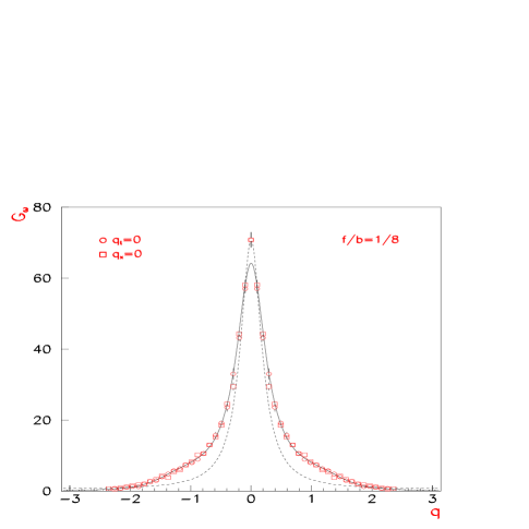
Figure 1: Scalar Propagator in momentum space in a $8_{8}$ lattice. The dash line is the fit to the free ansatz (40) at small momenta. The solid line corresponds to a fit to the inverse of a fourth order polynomial in $\hat{q}^{2}$.

In fact, if the interpolation was strictly local (i.e. the interpolated field in each $b$ plaquette depends only on the surrounding links), the correlation length of the $\omega$ fields at distances larger than $2b$ would vanish. In this case, it would not be appropiate to talk about a scalar mass. However, due to the fact that the group is compact, a smooth interpolation cannot be strictly local [4]. Empirically we find that the non-locality of the interpolation is nevertheless consistent with an exponential decay of the scalar propagator at large distances ($>2b$), with a mass of the order of the boson cutoff.

At large momentum, however, the $\omega$ propagator differs considerably from the free ansatz. Since the interpolation is smooth, the momentum modes higher than $q\sim f/b$ (boson cutoff) are expected to be suppressed for small $f/b$. Empirically, the inverse propagator at large momenta can be fitted for these lattice sizes to a polynomial in $\hat{q}^{2}$ of fourth order (solid line in Fig. 1). In Fig. 2, we show the large-momentum behaviour of the scalar propagator for two different values of the two-cutoff ratio $f/b$. Clearly, the high-momentum suppression increases as this ratio is decreased, as expected.

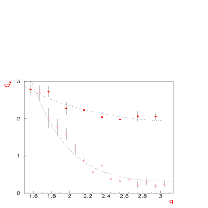
Figure 2: Scalar propagator in the large-momentum region for two values of $f/b=1/8$ (triangles), $1/4$ (circles). The curves are fits to the inverse of a fourth-order polynomial in ${\hat{q}}^{2}$ in the whole momentum range.

Concerning the condensates, there is also some difference with the OC case. The chirally breaking condensate,

$$v=\langle\;\frac{1}{L^{2}}\sum_{x}\omega(x)\;\rangle$$ (41)

is expected to be zero, since we are in the symmetric phase. Numerically, it is zero within statistical errors.

The condensate relevant for the strong phase,

$$z^{2}\equiv\langle\frac{1}{2L^{2}}\sum_{x,\hat{\mu}}{\mbox{R}e}[\;\omega(x)\omega^{\dagger}(x+\hat{\mu})\;]\rangle,$$ (42)

is plotted in Fig. 3 for two lattice sizes of $L/b=8,\;4$, as a function of the ratio $f/b$. It is easy to show from the explicit expression of the interpolated $\omega$ fields that,

$$\lim_{f/b\rightarrow 0}\;\;z^{2}=\;\;1$$ (43)

for fixed $L/b$. This is in contrast to what happens in the OC formulation, where $z^{2}=0$ for $\kappa=0$. This important difference between the OC and TC cases is not strange, since $z^{2}$ gets important contributions from short distances (as opposed to $v$, which only depends on the long-distance scalar dynamics) and the short-distance scalar dynamics is drastically modified by the interpolation.

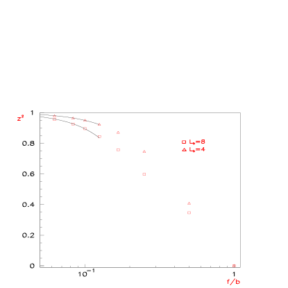
Figure 3: $z^{2}$ condensate for two lattice sizes $L/b=8,4$ as a function of the ratio $f/b$. The lines are quadratic fits.

One important question is what the volume dependence of these results is. Since the $\Omega$ fields are random at the scale $b$ we do not expect an important dependence on $L/b$ . We have computed the scalar propagators for various lattice sizes, and we find that the scalar “mass” (as obtained from the momentum fit (40)) is proportional to the ratio $f/b$, as expected. This means that the scalar mass in $b$ units does not depend on $f/b$. On the other hand, there is no clear dependence on $L/b$. This is shown in Table 1. In all the cases the scalar masses are of $O(1)$ in $b$-lattice units.

$f/b$	$L/b$	$m_{\omega}$ ($b$ units)
1/8	6	1.70(6)
	8	1.72(6)
	10	1.75(15)
1/4	8	1.69(6)
	10	1.54(10)

Table 1: Scalar mass in units of $b$ for various lattice sizes from momentum fits (40).

The volume dependence of the condensate $z^{2}$ is shown in Fig 3. For fixed $f/b$, there is some dependence on the volume. In order to keep $z^{2}$ constant, the infinite volume limit must be taken in a correlated way with the ratio $f/b$. A sensible way of taking the infinite volume limit might be by following lines of constant $z^{2}$ in the $(f/b,b/L)$ plane. From Fig. 3 we see that, according to this rule, $f/b$ does not need to decay as fast as $b/L$.

5.2 Fermion Spectrum

The fermion propagators have been obtained with the conjugate-gradient method for several lattice sizes and $y$ couplings. Since we are only interested in the regime where doublers are decoupled, we have kept the Wilson coupling fixed at $r=1$. According to the OC phase boundary $y+2r=O(1)$, we are then in the strong phase. As we will see, the strong phase in the TC has more structure, depending on the value of $y$.

The various propagators are given by

$$S_{ij}^{a}(t)=\langle\sum_{x_{1},y_{1}}\;\;\Psi_{i}^{(a)}(x)\bar{\Psi}_{j}^{(a)}(y)\;\;e^{ip_{1}(y_{1}-x_{1})}\;\;\rangle_{\Omega},\;\;\;\;\;t=|y_{2}-x_{2}|,$$ (44)

where $t=1,...,L$, the index $a$ refers to the neutral (n), charged (c) or physical (p) fermion for $p_{1}=0$, and the corresponding spatial doublers (nd), (cd) and (pd) for $p_{1}=\pi$. $i,j=R,L$ for the different chiralities. For every inversion the time slice at the origin $x_{2}$ is chosen randomly. The number of sampled scalar configurations is typically of $O(2-5\ 10^{2})$.

As in the OC construction, invariance of the action (26) under $PT$, i.e. a spatial and temporal inversion, implies

$$S^{a}(t)=-\gamma_{5}\;S^{a}(T-t)\;\gamma_{5},$$ (45)

which means that there is antisymmetry under $t\rightarrow T-t$ for the chirality-breaking components, RR and LL, and symmetry for the chirality-preserving ones, RL and LR. Notice that there is no symmetry under $T$ or $P$, since the action explicitly breaks parity.

In order to check that these symmetries are well satisfied we have monitored the behaviour $t<T/2$ and $t>T/2$ of the propagators. The expected $PT$ symmetry is well satisfied within statistical errors. If the low lying spectrum consists of free massive fermions, $P$ and $T$ symmetries are also expected to be satisfied effectively, while if the spectrum is chiral $P$ and $T$ are broken explicitely.

5.2.1 Large-$y$ Regime

At large $y\gg f/b$, we find that all the fermions are massive, as was also found in OC studies. Of course this phase has no physical interest since the fermionic states are more massive, $m\sim y$, than the scalars and this implies that there is no FNN regime to look at. All the particles, scalars and fermions, have masses of the order of the cutoff. In any case, it is interesting to look at this regime in order to compare with OC studies and to confirm that also in the two-cutoff formulation, for large Yukawa couplings, fermions are massive even if chiral symmetry is not broken.

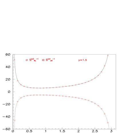
Figure 4: $(S^{(n)}_{RL,LR})^{-1}$ at $y=1.5$ and a lattice size of $8_{8}$. The solid lines correspond to the fits to the free Wilson fermion formulae of eq. (46). The parameters of the fits are given in Table 2.

Figure 4 shows the inverse neutral propagators in momentum space for $y=1.5$ in an $8_{8}$ lattice. The solid lines correspond to the fits to the free Wilson formula (for zero spatial momentum), i.e.

$${S^{(n)}_{LR,RL}(q)}^{-1}=\left[\;Z_{L,R}\;\frac{\sin q}{(\sin q)^{2}+(y_{eff}+r_{eff}(1-\cos q))^{2}}\;\right]^{-1}$$

$${S^{(n)}_{LL,RR}(q)}^{-1}=\left[\;Z_{LL,RR}\;\frac{y_{eff}+r_{eff}(1-\cos q)}{(\sin q)^{2}+(y_{eff}+r_{eff}(1-\cos q))^{2}}\;\right]^{-1}$$ (46)

with $Z_{LL,RR}=(Z_{L}Z_{R})^{1/2}$. All propagators can be fitted with a very good $\chi^{2}$ to the free Wilson propagator. The hopping expansion is a very good approximation at large momentum ($q>\pi/b$) as can be seen in Table 2. We present the results for $y_{eff}$ and $r_{eff}$ of the fits to (46), excluding the points near zero momentum, together with the result of the hopping expansion to first order (31). If the points near zero momentum are included in the fit the $\chi^{2}$ increases considerably, indicating that the free propagator (46) is not a good approximation in the low-momentum region.

This effect is more clearly seen in the behaviour of the propagators at large times.

y	Prop		RR	RL	LR	LL	Hopp.
1.	$S^{(n)}$	Z	1.084(5)	1.006(23)	1.175(19)	1.086(5)
		$y_{eff}$	1.090(6)	1.081(18)	1.087(11)	1.093(6)	1.085
		$r_{eff}$	1.081(6)	1.090(11)	1.083(8)	1.082(5)	1.085
	$S^{(nd)}$	Z	1.084(5)	0.992(26)	1.176(10)	1.085(5)
		$y_{eff}$	1.085(5)	1.064(14)	1.085(5)	1.086(5)	1.085
		$r_{eff}$	1.084(5)	1.086(14)	1.084(5)	1.085(5)	1.085
1.2	$S^{(n)}$	Z	1.082(5)	0.997(23)	1.172(11)	1.085(5)
		$y_{eff}$	1.304(5)	1.289(22)	1.301(6)	1.307(6)	1.302
		$r_{eff}$	1.080(5)	1.085(14)	1.082(5)	1.082(5)	1.085
	$S^{(nd)}$	Z	1.084(5)	0.969(32)	1.175(10)	1.085(5)
		$y_{eff}$	1.301(6)	1.266(20)	1.301(6)	1.302(6)	1.302
		$r_{eff}$	1.084(5)	1.072(20)	1.084(5)	1.085(5)	1.085
1.5	$S^{(n)}$	Z	1.084(4)	1.009(15)	1.175(8)	1.085(3)
		$y_{eff}$	1.630(6)	1.624(13)	1.628(5)	1.631(5)	1.627
		$r_{eff}$	1.082(4)	1.093(7)	1.083(4)	1.083(3)	1.085
	$S^{(nd)}$	Z	1.085(3)	0.991(25)	1.178(13)	1.085(3)
		$y_{eff}$	1.628(5)	1.608(19)	1.629(10)	1.628(5)	1.627
		$r_{eff}$	1.085(3)	1.083(13)	1.085(6)	1.085(3)	1.085

Table 2: Fits of the neutral propagators (light and doubler) in momentum space to the free Wilson formula for large $y$ in an $8_{8}$ lattice ($z^{-1}=1.085$).

In Fig. 5, we present the $LR$ component of the neutral propagator for two large values of $y$ together with the result from the momentum fits. Clearly, there is a systematic difference at large times, which only decreases slowly as $y$ increases. The time propagators can be very well approximated by a two-exponential fit, as shown in Fig. 5, but we do not have a deep understanding of the origin of the lighter states that seem to propagate at large times in this channel. What is clear from our data, however, is that at small times, typically $t<b-2b$, the propagators are very well reproduced by the hopping result and are thus dominated by the propagation of a free massive fermion. In the future we will explore the possibility that the deviations from the hopping result could be explained by the presence of fermion-scalar interactions. As explained in [8] an effective Lagrangian for the neutral field compatible with the global symmetry is

$${\cal L}_{eff}\rightarrow\bar{\Psi}^{(n)}(\not\!\partial+m_{n})\Psi^{(n)}+\lambda\;\bar{\Psi}^{(n)}_{L}\gamma_{\mu}\Psi^{(n)}_{L}(\omega\partial_{\mu}\omega^{\dagger}-\omega^{\dagger}\partial_{\mu}\omega).$$ (47)

OC studies did not find evidence for such interactions. In fact, when the fermions are much lighter than the scalar fields, this is to be expected from FNN arguments, since the scalars should decouple from the light spectrum, but when the fermions are more massive than the scalars as in our case, there is no reason to believe that these interactions are absent.

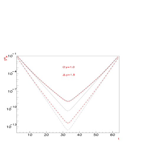
Figure 5: $S^{(n)}_{LR}$ propagators in time for $y=1,1.5$ and a $8_{8}$ lattice. The lines following the data points are the result of a two exponential fit. The dotted and solid lines, which deviate at large times, are the results of the momentum fits of Table 2.

The results for the neutral doubler are also shown in Table 2. As expected, there is good agreement with the hopping result in momentum space. The large-time behaviour of these propagators, however, also shows an anomalous behaviour: the effective mass at large times clearly decreases to a smaller value, see Fig. 6. In the case of the doublers, a scalar-fermion interaction of the form (47) means that the doubler is not stable. It can decay into a light mode and two scalars, since it is heavier. This coupling is quite weak because in such a decay the scalars carry large momenta and, as we have seen, the large Fourier modes of the scalar fields are strongly suppressed. Empirically, the overlap with the lighter states is very small: $Z\sim 10^{-6}$.

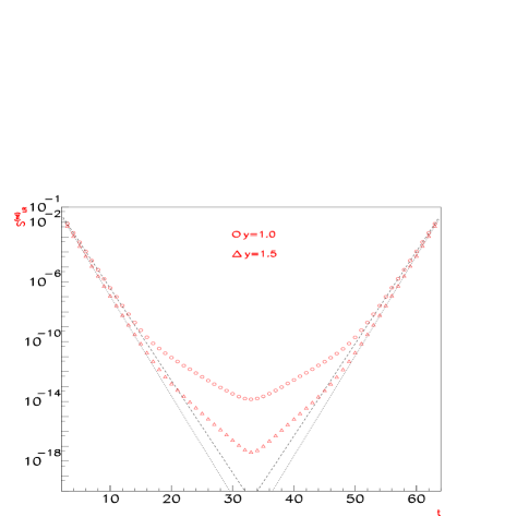
Figure 6: $S^{(nd)}_{LR}$ propagators in time for $y=1,1.5$ in a $8_{8}$ lattice. The dotted and dashed lines, which deviate at large times, are the results of the momentum fits of Table 2.

To summarize, we can conclude from our data that the first order hopping expansion provides a good approximation for the neutral propagators at large momenta and small times, in the large-$y$ region. At large times, the effective mass decreases and it is not clear whether there is an asymptotic free fermion in this channel. Notice that the FNN argument is not at work here, because the fermion mass is much larger than the scalar correlation length. In any case, the fact that the propagators are well reproduced by the hopping expansion at small times ($t<b-2b$) implies that, by choosing $f/b$ small enough, the correlations can get negligibly small at $t\sim b$ and are not expected to affect long-distance observables, if a light sector was present in the theory.

The charged propagators, both doubler and non-doublers, also behave as massive Dirac fermions. However, in this case the hopping approximation is not a good approximation even at small times. This is similar to what was found in OC studies. In Fig. 7 we show the RL components of the charged propagator, together with a two-exponential fit.

y	$m^{(n)}$ ($f$-units)	$m^{(c)}$ ($f$-units)
1.	0.538(4)	0.745(27)
1.2	0.653(7)	0.868(43)
1.5	0.816(3)	0.982(21)

Table 3: Effective masses from a single-exponential fit at large times of the neutral and charged $LR$ propagators for large $y$, for a lattice size of $8_{8}$.

In Table 3, we compare the effective masses obtained from a single-exponential fit in the large-time region of the neutral and charged $LR$ propagators. The difference between them is of the order of the scalar mass from Table 1. This is consistent with the charged propagator being a two-particle state, $\omega^{\dagger}\Psi^{(n)}$, as favoured by OC studies.

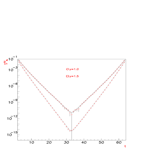
Figure 7: $S^{(c)}_{RL}$ propagators in time for $y=1,1.5$. The lines following the data points are the result of the two-exponential fits.

5.2.2 Small-$y$ Regime

As we decrease $y\leq 1$, the different chiral components of both the light neutral and charged propagators start to differ, signalling a violation of parity. Two components start getting lighter than the others: $S^{(n)}_{RL}=S^{(p)}_{RL}$ and $S^{(c)}_{LR}=S^{(p)}_{LR}$ (i.e. the expected physical fields). From our data we cannot establish a transition line in which parity violation shows up. It seems that the behaviour of the propagators changes in a smooth way, the violations of parity being present also at large $y$ and getting larger smoothly as $y$ is decreased.

There is, however, a critical value of $y_{c}$ below which the two lighter components $S^{(n)}_{RL}$ and $S^{(c)}_{LR}$ get actually massless at finite lattice spacing. This is the onset of the announced chiral phase. It is not clear what determines the value of $y_{c}$. There is one obvious candidate, which is the boson cutoff, i.e. $f/b$ in $f$-lattice units. Although our numerical results are not definite on this point, they seem to indicate that $y_{c}$ is related to this scale. The physical picture behind this expectation is nothing but the FNN conjecture that at distances larger than $b/f$ in $f$-units, the scalars should decouple. The correlation length of the light fermions in the strong phase is $\sim y$, so when $y<f/b$ the scalars decouple from the light fermions and a chiral phase appears.

As explained in the previous section, in order to study this phase, it is better to go to momentum space, where the limits $q\rightarrow 0,\pi$ of the propagator are known. In Fig. 8, we present the RL and LR components of the neutral and charged inverse propagators for $y=0.05$. Clearly the $S^{(n)}_{RL}=S^{(p)}_{RL}$ and $S^{(c)}_{LR}=S^{(p)}_{LR}$ propagators have poles only at $q\rightarrow 0$, as expected from massless undoubled fermions.

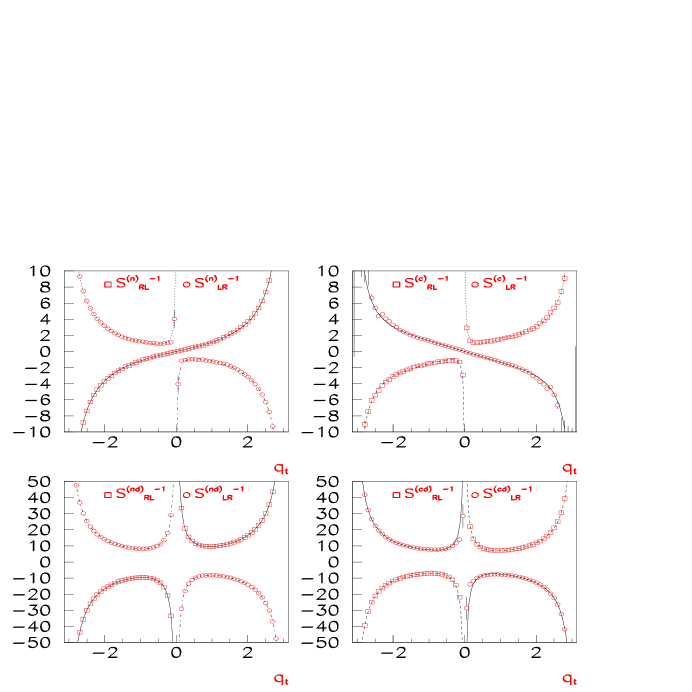
Figure 8: Inverse propagators $(S^{(n),(nd)})^{-1}$ and $(S^{(c),(cd)})^{-1}$ in momentum space in an $8_{8}$ lattice for $y=0.05$.

On the other hand, the components $S^{(n)}_{LR}$ and $S^{(c)}_{RL}$ show no poles, in agreement with them being two particle states composed of a massive scalar particle and a massless fermion (35).

In Fig. 9, we present a zoom of the massless components in the small momentum region for several values of $y$. The continuum curves are fits of the form (the spatial momentum being zero),

$$S^{(n,c)}_{RL,LR}(q)=\frac{Z_{R,L}}{\sin(q)}+Z^{\prime}_{R,L}\frac{\sin(q)}{\sin(q)^{2}+{m^{\prime}}_{R,L}^{2}}.$$ (48)

The second term corresponds to higher states, which should decouple in the continuum limit. Their masses are expected to be of the order of the boson cutoff or larger. It is clear from the figures that the contamination of the charged chiral mode is larger than that of the neutral one.

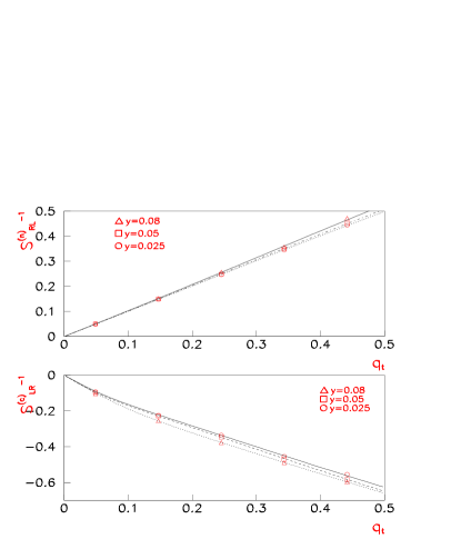
Figure 9: $(S^{(n)}_{RL})^{-1}$ and $(S^{(c)}_{LR})^{-1}$ at small momentum for several values of $y$ in the chiral phase.

We show the results of these fits for several lattice sizes in Table 4.

Size	$Z_{R}$	$Z_{L}$	$m^{\prime}_{L}$ ($b$-units)	$\frac{Z^{\prime}_{L}}{Z_{L}}$
$6_{6}$	0.994(1)	0.543(12)	1.16(17)	0.384(25)
$6_{8}$	0.994(1)	0.668(17)	1.27(34)	0.257(23)
$8_{4}$	0.994(3)	0.168(33)	0.95(22)	2.245(54)
$8_{8}$	0.996(1)	0.494(21)	1.08(13)	0.603(84)
$10_{8}$	0.995(1)	0.485(40)	1.22(44)	0.52(12)

Table 4: $Z_{L,R}$, $Z^{\prime}_{L}/Z_{L}$ and $m^{\prime}_{L}$ for various lattice sizes. $y$ is kept fixed to $0.2$ in units of $b$.

The volume effects as $L/b$ changes, for fixed $f/b$, are quite small and it seems clear that the contaminating mass $m^{\prime}$ does not decrease as the volume is increased. On the other hand, for fixed $L/b$, the contamination increases considerably for the charged propagator, when the cutoff ratio is increased.

In Fig. 10, we zoom the low-momentum behaviour of $S^{(n)}_{LR}$ and $S^{(c)}_{RL}$. It is important to make sure that these propagators do not develop poles as $y$ gets smaller or as the continuum limit is approached, rendering the theory vector-like. It is not clear how to fit these propagators at zero momentum, since they are expected to be multiparticle states. We have used the simplest ansatz,

$$S^{(n,c)}_{LR,RL}(q)=\tilde{Z}_{L,R}\frac{\sin(q)}{\sin(q)^{2}+(m^{(n,c)}_{L,R})^{2}},$$ (49)

which empirically gives a good fit near $q=0$. In Table 5, we present the masses obtained from these fits for various lattice sizes.

Size	$m^{(n)}_{L}$ ($b$ units)	$m^{(c)}_{R}$ ($b$ units)
$6_{6}$	2.26(11)	2.08(78)
$6_{8}$	2.19(14)	2.03(11)
$8_{8}$	2.46(13)	2.32(10)
$10_{8}$	2.59(51)	2.03(19)

Table 5: $m^{(c)}_{R}$ and $m^{(n)}_{L}$ from a fit to (49) for various lattice sizes, in units of the boson cutoff $b^{-1}$; $y$ is kept fixed to $0.2$ in $b$ units.

It is clear that these masses are of the order of the boson cutoff, as expected from (35). Also, there is no sign of the masses getting smaller as the volume increases or as $y$ is decreased.

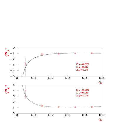
Figure 10: $(S^{(n)}_{LR})^{-1}$ and $(S^{(c)}_{RL})^{-1}$ at small momentum for several values of $y$ in the chiral phase. The lines are fits to (49), which give $m^{(n)}_{L}=2.46(13),2.46(35),2.10(55)$ and $m^{(c)}_{R}=2.32(10),2.19(21),2.07(29).$, in increasing order of $y$.

For the neutral doublers, we find that the large-momentum ($q>\pi/b$) and small-time ($t<b$) behaviour corresponds to that of a free massive fermion, which supports the picture that, due to the strong coupling between the doubler modes and the scalars, the neutral composite fermion (25) is formed. In Table 6, we present the fits of the neutral doubler inverse propagators to the free Wilson formulae for large momentum ($q>\pi/b$). The effective $r$ is in perfect agreement with the hopping result. The effective $y$ on the other hand differs (especially for the RL component). This could be due to a low-momentum bias, since the hopping result is not a good approximation for momenta of the order of the boson cutoff.

y	Prop		RR	RL	LR	LL	Hopp.
0.025	$S^{(nd)}$	Z	1.083(6)	0.992(16)	1.173(8)	1.087(3)
		$y_{eff}$	0.033(5)	0.004(4)	0.030(4)	0.033(1)	0.027
		$r_{eff}$	1.082(5)	1.090(8)	1.082(4)	1.086(3)	1.085
0.05	$S^{(nd)}$	Z	1.084(5)	0.993(16)	1.173(8)	1.087(2)
		$y_{eff}$	0.061(3)	0.024(4)	0.057(1)	0.059(5)	0.054
		$r_{eff}$	1.082(4)	1.090(8)	1.082(4)	1.086(3)	1.085
0.08	$S^{(nd)}$	Z	1.082(4)	0.997(17)	1.172(8)	1.087(4)
		$y_{eff}$	0.092(1)	0.056(5)	0.089(1)	0.092(1)	0.087
		$r_{eff}$	1.081(4)	1.092(8)	1.082(4)	1.086(4)	1.085

Table 6: Fits of the neutral doubler propagators in momentum space ($q>\pi/b$) to the free Wilson formula for small $y$ in an $8_{8}$ lattice.

At large times or small momenta, there is evidence of contamination from lighter states, which are probably multiparticle states. This is not so surprising since the neutral composite is not expected to be stable in this phase. Possible effective interactions, compatible with the symmetries that connect the light and doubler sectors are given by

$$g_{n}\;\{\;\bar{\Psi}^{(p)}\omega^{\dagger}P_{R}\;\partial_{\mu}^{2}\Psi^{(nd)}+\bar{\Psi}^{(nd)}\partial_{\mu}^{2}(\omega P_{L}\Psi^{(p)})\;\}.$$ (50)

In the presence of these interactions, the neutral doubler channel $S^{(nd)}_{RL}$ at large times will be dominated by two-particles states. The decay of the neutral doublers into lighter particles however involves high momentum modes of the scalar field, which are suppressed for TC, so we expect that they are relatively long-lived and thus dominate the propagators at small times. Notice that in the OC case, this does not have to be the case.

In Fig. 11 we present the effective masses in the $RL$ and $LR$ neutral and charged doubler channels for $t<b-2b$, for three values of $L/b$ and fixed $f/b$. The neutral effective mass has a nice plateau at small times. This is consistent with the assumption that this channel is dominated by the neutral composite of (25). On the other hand, the charged doubler does not show a plateau. The effective mass is of the order of the fermion cutoff at small times, but it is nowhere constant. This indicates that the charged doubler composite is not formed and multiparticle states are dominating this channel.

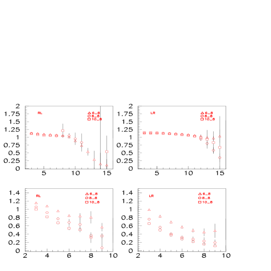
Figure 11: Effective mass of the neutral (up) and charged (down) doublers for several lattice sizes and $y=0.025$.

Although our statistics is not good enough to attempt a quantitative description of the doubler propagators at large times, the fact that, at small times $t<b-2b$, the propagators decay as particles with masses of the order of the fermion cutoff implies that, after a few $f$-time slices, the correlation in the doubler channels is too small to influence the long-distance physics. In the simplified model we are considering here there is no more long-distance physics than the free propagation of massless fermions. In Figs. 13 and 14, we compare the decay in time of the various propagators, neutral and charged respectively, for several lattice sizes. The massless components have constant correlation as expected. All the remaining propagators are not simple at large times, but they are clearly split from the light sector. For $f/b=1/8$, they are suppressed by at least 2–3 orders of magnitude. We notice that the effect of increasing $f/b$ is quite dramatic for the charged propagator (see last figure in Fig. 14). In general the splitting between the doubler and non-doubler sectors is larger for the neutral channel.

To summarize, we have found that at small enough $y$ there is a chiral phase, in which the light spectrum consists of two massless fermions with chiral quantum numbers. Their propagators in momentum space show only one pole at $q\rightarrow 0$, as expected from undoubled massless particles. The neutral doubler channel seems to be dominated by a massive fermion at small times, while at large times it is probably dominated by multiparticle states. The charged doubler channel seems to be everywhere dominated by multiparticle states. These states contain scalars, whose correlation length is of the order of the boson cutoff $b^{-1}$; thus they are expected to decouple in the continuum limit. In order to show that this is indeed the case, it will be necessary to consider the case where gauge interactions are switched on, since only in this case is there a physical mass gap that can be used to define the continuum limit of the lattice model. We have not found important volume effects as $L/b$ is increased, although there is a clear dependence on $f/b$: the splitting between the light sector and the heavy one becomes smaller as $f/b$ is increased. This is a clear indication of the importance of the cutoff separation.

We have not analysed in detail the intermediate region of couplings $y_{c}<y<O(1)$, and in particular, we have not addressed the important issue of the nature of the transition at $y_{c}$. More statistics will be needed for this. However, we have monitored one observable that has proved useful in the location of crossover or transition lines in previous studies of Wilson-Yukawa models [1]. This is simply the number of conjugate-gradient iterations (NCG) needed in the propagator inversion for a fixed precision. The naive expectation is that the required number of iterations should increase as $y$ decreases, because the lowest eigenvalue of the fermion matrix decreases with $y$. This changes however when we enter the chiral phase, since the light mode is massless and the lowest eigenvalue is fixed by the IR cutoff, which is the lowest lattice momentum (remember we use AP boundary conditions in the time direction). Thus the number of iterations should not keep increasing for $y<y_{c}$. In Fig. 12, we show the NCG for different values of $y$. There seems to be a maximum very close to the value where we believe $y_{c}$ should be, according to the behaviour of the propagators.

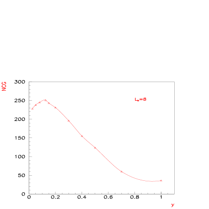
Figure 12: Number of conjugate-gradient iterations in the inversion of the neutral propagator as a function of $y$ in an $8_{8}$ lattice.

The position of the maximum is in fact near $y=0.15$ in $f$ units, which is not far from $f/b=1/8$, as naively expected.

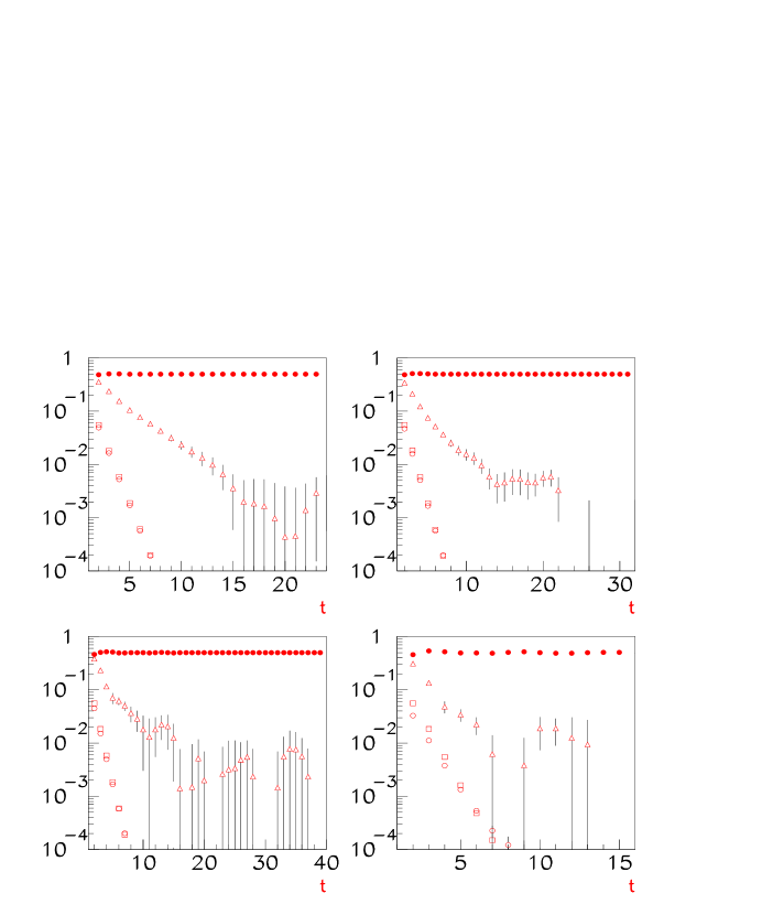
Figure 13: $S^{(n)}_{RL}$ (full circles), $S^{(n)}_{LR}$ (triangles), $S^{(nd)}_{RL}$ (circles), $S^{(nd)}_{LR}$ (squares) for several lattice sizes: $6_{8}$, $8_{8}$, $10_{8}$ and $8_{4}$, for $y=0.025$.

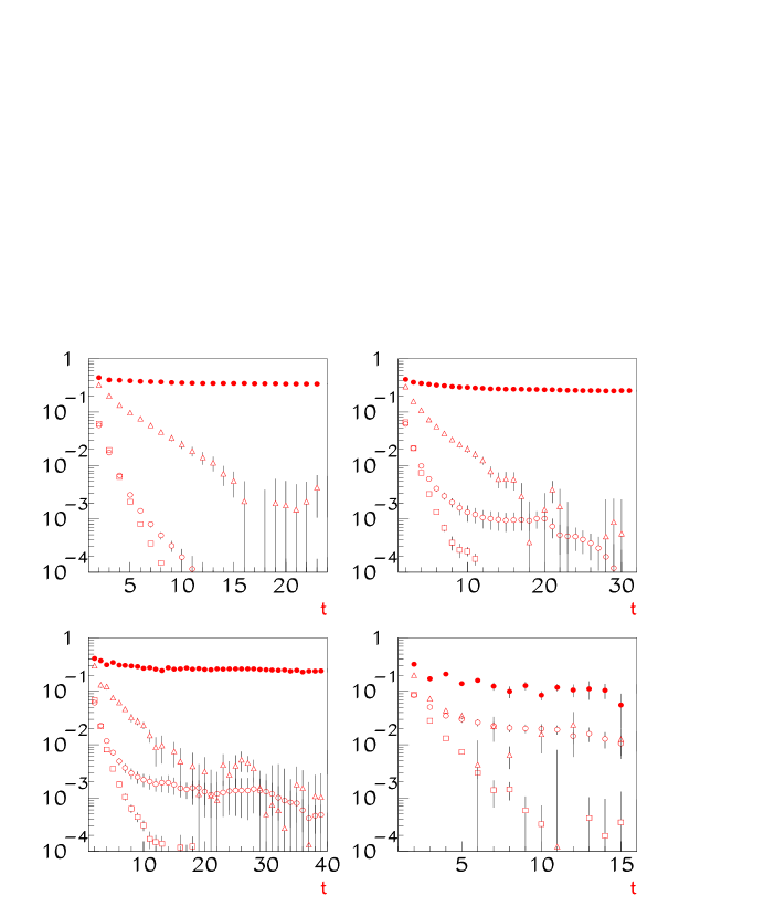
Figure 14: $S^{(c)}_{LR}$ (full circles), $S^{(c)}_{RL}$ (triangles), $S^{(cd)}_{LR}$ (circles), $S^{(cd)}_{RL}$ (squares) for several lattice sizes: $6_{8}$, $8_{8}$, $10_{8}$ and $8_{4}$, for $y=0.025$.

6 Effects of unquenching

It is clear that unquenching in the OC case can have dramatic effects. By naive power counting, fermion loops can induce $O(1)$ corrections to the potential of the $\omega$ fields. In order to be in the FNN regime, tunings of $\kappa$ and probably other relevant operators of dimension 4 that are generated at higher orders might be needed.

As explained in [3], in the TC case the situation is very different. Due to the suppression of the high-momentum modes of the scalar fields, it can be shown that the corrections induced by fermion loops on the scalar potential are down by powers of the two-cutoff ratio, $O(f/b)^{2}$. For this reason it is expected that unquenching is not going to change the phase diagram of the fermion-scalar model in any important way. A way to quantify this is by looking at how the phase of the fermion determinant for the action (14) changes under a gauge transformation. The magnitude of this change is a measure of the strength of the couplings of the scalar fields $\omega$, induced by the fermion loops. At this stage, however, we have to enlarge the fermion content of the model we are considering in order to cancel gauge anomalies. Otherwise the changes in the phase are of $O(1)$ and the two-cutoff method is of no use, nor any other, of course. A simple choice is the $11112$ model, with four left-handed fermions with $U(1)$ charge $q_{L}=1$ and one right-handed fermion with charge $q_{R}=2$. Gauge anomalies cancel, because

$$\sum_{i}q^{2}_{i,L}=\sum_{i}q^{2}_{i,R}.$$ (51)

In Fig. 15, we present a histogram of the change in the phase of the fermion determinant in a lattice of $L/b=4$ and several values of $f/b=1,1/4,1/8$, under a random $b$-lattice gauge transformation, starting from the trivial configuration. As expected, the change in the phase of the fermion determinant gets smaller with the ratio $f/b$. For arbitrarily small $f/b$, it is clear that the FNN conditions are still satisfied in the full theory. A full unquenched simulation would be needed to determine how small this ratio has to be in practice.

Fermion loops are also expected to induce renormalization of the Yukawa couplings $y$ and $r$ at higher orders. For the same reason as before, it can be shown [3] that the corrections to these couplings are down by powers of $(f/b)^{2}$. Thus, for small enough $f/b$, no tunning of the bare Yukawa couplings is needed to remain in the chiral phase.

Figure 15: Change in the phase of the fermion determinant under random gauge transformations in lattice sizes $4_{1}$, $4_{4}$ and $4_{8}$.

7 Conclusions

We have presented numerical evidence in favour of the existence of a truly chiral phase in a two-cutoff formulation of a quenched 2D Wilson-Yukawa model with a global $U(1)_{L}\times U(1)_{R}$. The Yukawa phase diagram is different from the one found in the one-cutoff formulation of this model in that there is a new phase for $r=O(1)$ and $y\ll 1$, where doublers are split from the light spectrum, which is composed of massless fermions with chiral quantum numbers. When one of the chiral symmetries is gauged, the continuum limit of this lattice model is expected to give rise to a chiral gauge theory.

The main new feature of the two-cutoff formulation is that the high Fourier modes of the scalar fields are naturally cut off at a scale smaller than the momenta of the fermion doublers. As a consequence the Wilson-Yukawa term is truly a perturbative coupling for the ligh-fermion mode ($p\rightarrow 0$), while it is effectively a large $O(r)$ Yukawa coupling for the doubler modes ($p\rightarrow\pi$). Near $p\rightarrow 0$, the chiral fermion propagators are well reproduced by weak Yukawa perturbation theory and have poles at $p\rightarrow 0$, while at large momenta they are better described by the strong Yukawa expansion, which predicts no doubler poles (since all fermions are massive in this approximation).

All our results have been obtained in the symmetric or VX phase (PM in 4D) of the scalar dynamics. This is the relevant phase for describing a chiral gauge theory. In the case of a spontaneously broken gauge theory in 4D, the relevant phase would be a ferromagnetic (FM) one. If a FM counterpart of the chiral phase found here exists, it would lead to a successful discretization of the Standard Model. This interesting case will be considered elsewhere.

Acknowledgements We thank J.L. Alonso, M.B. Gavela, M. Guagnelli, K. Jansen, R. Sundrum, M. Testa and T. Vladikas for very helpful discussions/suggestions. LPTHE is laboratoire associé au CNRS.

Appendix A.

We present here the explicit formulae for the compact $U(1)$ interpolation in 2D. For details on how to construct this interpolation the reader is referred to [4]. The methods are similar to those used in [13].

The $b$-lattice sites are denoted by $s$. For an arbitrary gauge configuration on the $b$-lattice, we can uniquely write each lattice link variable in the form

$$U_{\mu}(s)=e^{iA_{\mu}(s)},~{}~{}|A_{\mu}(s)|<\pi,$$ (A. 1)

where we are neglecting the measure-zero set of lattice fields, where at least one of the link variables equals exactly $-1$. This assignment defines an obvious logarithm function for group elements different from $-1$:

$$A_{\mu}=-i\log U_{\mu},~{}~{}|A_{\mu}|<\pi.$$ (A. 2)

The link variables on the $f$-lattice can also be writen as

$$u_{\mu}=e^{ia_{\mu}},~{}~{}|a_{\mu}|<\pi.$$ (A. 3)

Defining the $f$-lattice sites within each $b$-lattice plaquette as $x=s+t_{1}\hat{1}+t_{2}\hat{2}$, where $0\leq t_{1},t_{2}\leq 1$, the final result is,

$$a_{1} = \frac{f}{b}\;\{\;(1-\;t_{2})\;(A_{1}(s)-2\pi N_{2}(s))+t_{2}\;(A_{1}(s+\hat{2})-2\pi N_{2}(s+\hat{2}))\;\}$$

$$a_{2} = \frac{f}{b}\;\{\;(1-\;t_{1})\;(A_{2}(s)+2\pi N_{1}(s))+t_{1}\;(A_{2}(s+\hat{1})+2\pi N_{1}(s+\hat{1}))\;\}$$ (A. 4)

Notice that the fields at the boundary of the plaquette satisfy $a_{\mu}=f/b\;A_{\mu}$.

Except for the contribution of the $N_{\mu}$ fields, this is simply a linear interpolation, as naively expected. The $N_{\mu}$ fields are integers defined by the following equation:

$$\sum_{\mu}\;\;N_{\mu}(s+\hat{\mu})-N_{\mu}(s)=N(s)$$ (A. 5)

where $N(s)$ are the winding numbers of the $a_{\mu}$ field defined on the boundary of the plaquette (to be more precise the winding of the $f\rightarrow 0$ limit of $a_{\mu}$ on the boundary), i.e.

$$I[\frac{A_{2}(s)+A_{1}(s+\hat{2})-A_{2}(s+\hat{1})-A_{1}(s)}{2\pi}]$$ (A. 6)

with $I[y]\equiv$ nearest integer to $y$. The existence of these fields is of course related to the compactness of the group. In particular, the geometrical definition of topological charge is simply given by, $\sum_{s}N(s)$. In this paper we are only concerned with topologically trivial configurations since $g=0$. Even in the case of trivial topology, a non-measure zero set of lattice configurations will have $N(s)\neq 0$. The number of non-zero windings grows with the $b$-lattice volume.

Equation (A. 5) has a unique solution in the “gauge” depicted in Fig. 16.

Figure 16: “Gauge” choice used in solving (A. 5) for compact $QED_{2}$. The $N_{\mu}$ corresponding to links that are not intersected by the path are zero.

All the links that are not crossed by the path have the associated $N_{\mu}(s)$ set to zero (remember that $\hat{\mu}$ is $orthogonal$ to the link in our notation). In order to ensure the discrete lattice symmetries, however, we have to also consider the interpolations obtained in the maximal gauges that are obtained from that in Fig. 1 by lattice symmetry transformations (i.e. $90^{\circ}$ rotations and temporal and spatial inversions). There are eight of these maximal trees in total. Ideally, the maximal path could be chosen randomly for each $b$-lattice configuration. This is however more complicated to implement, so we have used the first method.

We also need the interpolation of $b$-lattice gauge transformation, defined as

$$u[U^{\Omega}](x)=u^{\omega}[U](x),$$ (A. 7)

but in the simpler global limit, i.e.

$$u[I^{\Omega}](x)=u^{\omega}[I](x)=I^{\omega}(x),$$ (A. 8)

where $I$ is the identity configuration, i.e. $U_{\mu}(s)=1$ or $u_{\mu}(x)=1$. For the prescription (A. 4), there is a unique solution for $\omega$. Defining

$$\Omega(s)\equiv e^{i\Phi(s)},\;\;\;\;\;\omega(x)\equiv e^{i\phi(t_{1},t_{2})},$$ (A. 9)

the solution is,

$$\phi(t_{1},t_{2})=\Phi(s)+(A_{1}(s)-2\pi N_{2}(s))\;t_{1}+(A_{2}(s)+2\pi N_{1}(s))\;t_{2}$$

$$+(A_{2}(s+\hat{1})+2\pi N_{1}(s+\hat{1})-A_{2}(s)-2\pi N_{1}(s))\;t_{1}t_{2}$$ (A. 10)

with

$$A_{\mu}\equiv-i\log(\Omega^{\dagger}(s)\Omega(s+\hat{\mu})),~{}~{}|A_{\mu}|<\pi,$$ (A. 11)

and the $N_{\mu}$ fields are defined by (A. 5), (A. 6) and (A. 11).

It is easy to see that $\phi(0,0)=\Phi(s)$ and $\omega$ is thus a smooth interpolation of the gauge transformation $\Omega$.

References

-
[1]
J. Smit, Nucl. Phys. B (Proc. Suppl.) 9 (1989) 579. S. Aoki, I.H.
Lee and S-S. Xue, Phys. Lett. B229(1989) 403. S. Aoki, I.H.
Lee, J. Shigemitsu and R.E. Shrock, Phys. Lett. B229(1989) 403. S. Aoki, I.H.
Lee and R.E. Shrock, Nucl. Phys. B355(1991) 383. W. Bock et al., Phys. Lett. B232(1989) 486. I.M. Barbour et al., Nucl. Phys. B368(1992) 390. M.F.L. Golterman,
D.N. Petcher and J. Smit, Nucl. Phys. B370(1992) 370. W. Bock et al., Nucl. Phys. B371(1992) 683. W. Bock, A.K. De, and J. Smit, Nucl. Phys. B388(1992) 243. - [2] For a review and references on this subject see Nucl. Phys. B(Proc. Suppl.)29B,C(1992) 83.
- [3] P. Hernández and R. Sundrum, Nucl. Phys. B455(1995) 287.
- [4] P. Hernández and R. Sundrum, Nucl. Phys. B472(1996) 334.
- [5] A. Borrelli et al., Nucl. Phys. B333(1990) 335-356. L. Maiani, G.C. Rossi and M. Testa, Phys. Lett. B292(1992) 397.
- [6] D. Foester, H.B. Nielsen and M. Ninomiya, Phys. Lett. B94(1980) 135.
- [7] S.A. Frolov and A.A. Slavnov, Nucl. Phys. B411(1994) 647; A.A. Slavnov, Phys. Lett. B319(1993) 231.
- [8] W. Bock, A.K. De, E. Focht and J. Smit, Nucl. Phys. B333(1990) 335-356.
- [9] M. Golterman and D. Petcher, Phys. Lett. 225(1989) 159 and Nucl. Phys. B359(1991) 91.
- [10] M.F.L. Golterman, D.N. Petcher and E. Rivas, Nucl. Phys. B377(1992) 405.
- [11] V.L. Berezinskii, Sov. Phys. JEPT 32 (1970) 493. J.M. Kosterliz and D.J. Thouless, J. Phys. C6 (1973) 1181. J.M. Kosterliz, J. Phys. C7 (1974) 1046.
- [12] E. Witten, Nucl. Phys. B145(1978) 110.
- [13] M. Lüscher, Commun. Math. 85, 39-48 (1982). M. Göckeler, A. Kronfeld, G. Schierholz and U.J. Wiese, Nucl. Phys. B404(1993) 839-582.