1 Introduction

There is an ongoing effort to find improved lattice actions for asymptotically free theories like QCD that are nearly free of lattice artifacts by the means of renormalization group theory [2, 3]. The conceptual basics have been developed by Hasenfratz and Niedermayer for the $O(3)$ non-linear $\sigma$-model [1]. A good description of the basic ideas of improved lattice actions can be found in [9]. While using the renormalization group transformation (RGT) to get improved actions, it is important to understand the basic convergence properties of the transformation in the vicinity of the fixed point. In the standard way of thinking, the eigenvalues of the RG transformation can be determined by dimensional analysis. However, general RG transformations result in additional non-canonical eigenvalues. In this paper we give an insight how this mechanism works. Here we consider free fermionic field theories although the statements are more general.

The standard terminology is the following: For fermions, when we transform a fine lattice to a coarse one, we have

$$e^{-S^{\prime}[\bar{\Psi}^{\prime},\Psi^{\prime}]}=\int{\cal D}\bar{\Psi}\,{\cal D}\Psi\,e^{-S[\bar{\Psi},\Psi]-T[\bar{\Psi},\Psi;\bar{\Psi}^{\prime},\Psi^{\prime}]}$$ (1)

where $\bar{\Psi},\Psi$ and $\bar{\Psi}^{\prime},\Psi^{\prime}$ are the fermion fields on the fine and coarse lattice and $T$ defines the renormalization group or block transformation that does the averaging. In principle, there are no restrictions to $T$. But we want to choose an averaging that matches our intuitive picture of the renormalization group transformation. That means that we do not want $T$ to average over too much or too few sites on the fine lattice, just enough to account for the space between the coarse lattice points. It turns out that the interaction range of the FP action depends significantly on the actual choice of $T$.

Apart from these qualitative restrictions, one of the constraints that applies to $T$ is that the generating functional $Z$ (and thus the free energy and thermodynamics) should not change:

$$Z\;=\;\int{\cal D}\bar{\Psi}\,{\cal D}\Psi\,\exp\left\{-S[\bar{\Psi},\Psi]\right\}\quad=\;\int{\cal D}\bar{\Psi}^{\prime}\,{\cal D}\Psi^{\prime}\,\exp\left\{-S^{\prime}[\bar{\Psi}^{\prime},\Psi^{\prime}]\right\}$$ (2)

The long-distance properties are thus untouched. The correlation length measured in lattice spacings (the dimensionless counterpart of the physical correlation length; $\xi=\xi^{\mbox{\tiny phys}}/a$) is changed to $\xi/n$ since the lattice spacing is changed $a^{\prime}=na$ and thus $\xi^{\prime}=\xi/n$. In this work we only use transformations with $n=2$.

2 The RGT, its Operators and Fixed Points

2.1 Eigenoperators and Eigenvalues of the RGT

The action $S^{\prime}[\bar{\Psi}^{\prime},\Psi^{\prime}]$ is most generally a sum of all kinds of interaction terms even if $S[\bar{\Psi},\Psi]$ had a simple form. If we set the initial $S$ to the general form

$$S[\bar{\Psi},\Psi]=-\sum_{i}c_{i}X_{i}[\bar{\Psi},\Psi]$$ (3)

where $c_{i}$ denotes the couplings of the different interactions $X_{i}[\bar{\Psi},\Psi]$ ($i$ is just a labeling index). The interactions may be of any form conformal to lattice symmetries. These can be higher derivatives and higher powers of the fields $\bar{\Psi},\Psi$. The couplings $c_{i}$ form a coupling space. An RG transformation is moving the action in this space, and for very special sets of couplings $c_{i}^{\ast}$ the RG reproduces the same couplings – we have a fixed point FP of the RGT. In such FPs we have collective behavior over infinite many lattice sites. In the vicinity of the FP-set of couplings $\{c_{i}^{\ast}\}$ the function $c_{i}^{(n+1)}(c_{j}^{(n)})$ is given by

$$c_{i}^{(n+1)}(c_{j}^{(n)}) \!\!\!\!=\!\!\!\! c_{i}^{(n+1)}(c_{j}^{\ast})\!+\!\frac{\partial c_{i}^{(n+1)}}{\partial c_{j}^{(n)}}\!\!\left(\!c_{j}^{(n)}\!\!-c_{j}^{\ast}\!\right)\!+\!\cdot\!\!\cdot$$

(4)

So because $c^{\ast}$ is a FP, $c_{i}^{(n+1)}(c_{j}^{\ast})=c_{i}^{\ast}$ we have

$$\Delta c_{i}^{(n+1)}=R_{ij}\Delta c_{j}^{(n)}$$ (5)

where the $\Delta$ denotes the difference of the point $c$ to $c^{\ast}$. The procedure that follows is the usual one for a linearized symmetry: we try to identify its eigenvectors and eigenvalues. Denote the eigenvalues with $e_{\alpha}$ and the eigenvectors with $\sigma_{\alpha}$. The eigenvectors $\sigma_{\alpha}$ are some linear combinations of the operators $X_{i}$. The neighborhood of the FP can be then expressed as

$$S[\bar{\Psi},\Psi]=S^{\ast}[\bar{\Psi},\Psi]+\sum_{\alpha}d_{\alpha}\sigma_{\alpha}[\bar{\Psi},\Psi]$$ (6)

Performing one RG step we get

$$S^{\prime}[\bar{\Psi},\Psi]=S^{\ast}[\bar{\Psi},\Psi]+\sum_{\alpha}e_{\alpha}d_{\alpha}\sigma_{\alpha}[\bar{\Psi},\Psi]$$ (7)

If we continue to apply the blocking step to this action, we will get an additional factor $e_{\alpha}$ for each step. Of course this action will only converge towards $S^{\ast}$ if every eigenvalue $e_{\alpha}$ in the sum is smaller than $1$. Eigenvectors with such eigenvalues are called irrelevant. The most general action $S$ will have of course eigenvector-components with (relevant) eigenvalues larger than $1$ and thus the repeated application of the RG transformation will bring the system away from the FP. In order to converge to the FP, the coefficients $d_{\alpha}$ have to be set to zero for every relevant eigenvector $\sigma_{\alpha}$.

2.2 Redundant Operators

For the Gaussian Fixed Point, one can give the form of the eigenoperators and eigenvalues explicitly for specific RG transformations. The eigenvalues are depending of the engineering dimensions of the operators involved. They are all some exponent of $2$: We have $e_{\alpha}=1,\frac{1}{2},\frac{1}{4},\frac{1}{8},\ldots$

If we have some general RG transformation, one would think that the eigenvalues should be reproduced, and that specifically there is no eigenoperator with an eigenvalue $1/2<e_{\alpha}<1$ because it is impossible to write a regular operator with such an engineering dimension.

What we are seeing in the calculations, however, is that we do measure such eigenvalues. These eigenoperators with an eigenvalue between $1/2$ and $1$ are interpreted as redundant directions in the critical surface, i.e. connecting lines between possible FP actions. That’s why these eigenvalues have no physical significance. To be specific, we move on such a direction from a FP1 of a RG transformation (RG1), to FP2 of some other RG transformation (RG2) which is very similar to RG1. The ’difference’ between one transformation and the other one is giving the redundant operator and the eigenvalue may be in principle any number. If we are in the FP1 of RG1 and now apply RG2, we are moving towards FP2 with such a redundant eigenvalue. If this eigenvalue is smaller than $1$, we will eventually end up in FP2. If this eigenvalue is greater or equal $1$, this means that we cannot move from FP1 to FP2 since FP1 does not lie in the attracting region of FP2. In particular, if the eigenvalue is exactly $1$, then the points on the line between FP1 and FP2 will not move under RG1 or RG2 at all – the FPs of these transformations are not unique. This fact does not matter for continuum physics, because every point on the connecting line leads to an action which is describing the same theory.

Operators belonging to such directions are redundant, their presence in the action does not influence the lattice artifacts. Those are only influenced by the irrelevant operators.

2.3 The Blocking Function $T$ and the FP

Consider some lattice regularization of the maselss free fermionic theory:

$$S[\bar{\Psi},\Psi] = \sum_{q}\bar{\Psi}(q)\,\Delta(q)\,\Psi(-q)$$ (8)

$$\Delta(q) = \rho_{\mu}(q)\gamma_{\mu}+\lambda(q)$$ (9)

Usually, $T$ is written as

$$T[\bar{\Psi},\Psi;\bar{\Psi}^{\prime},\Psi^{\prime}]\;=\;\hskip 284.52756pt$$

$$\kappa\,\sum_{n_{\scriptscriptstyle\!\!B}}\left(\bar{\Psi}^{\prime}(n_{\scriptscriptstyle\!\!B})-b\,\sum_{j}\,\omega^{\dagger}(j)\bar{\Psi}(2n_{\scriptscriptstyle\!\!B}+j)\right)\left(\Psi^{\prime}(n_{\scriptscriptstyle\!\!B})-b\,\sum_{j}\,\omega(j)\Psi(2n_{\scriptscriptstyle\!\!B}+j)\right)$$ (10)

The function $\omega(j)$ is normalized and determines the exact form of the block transformation ( $\sum_{j}\omega(j)=1$ ). The integral over $\bar{\Psi}$ and $\Psi$ in (1) is a Gaussian integral and it is easily carried out. The action after one RG transformation has the form

$$S^{\prime}[\bar{\Psi}^{\prime},\Psi^{\prime}]=\sum_{Q}\bar{\Psi}^{\prime}(Q)\,\Delta^{\prime}(Q)\,\Psi^{\prime}(-Q)\\$$ (11)

$$\Delta^{\prime-1}(Q)=\frac{1}{\kappa}+\frac{b^{2}}{2^{d}}\sum_{\ell=0}^{1}\Delta^{-1}\left(\frac{Q}{2}+\pi\ell\right)\left|\,\omega\left(\frac{Q}{2}+\pi\ell\right)\right|^{2}$$ (12)

This is our new effective action for the coarser lattice. The initial action can be in principle any fermionic action of the same quadratic form. Here $Q$ is the coarse-lattice momentum and $d$ counts the dimensions (usually $d=4$). This expression is very convenient for iterative purposes. The iteration can be carried out for the inverse of the action kernel (i.e. the propagator). Since $\Delta(q)$ has a simple matrix structure (8) the inversion $\Delta^{-1}(q)$ to get the propagator is easy and the recursion straightforward, giving the same matrix structure $(\alpha_{\mu}\gamma_{\mu}+\beta{\bf 1})$. Having found a recursion relation for the propagator $\Delta^{-1}$, we can invert it back to get the new action kernel. Then we can iterate the action $S$ to obtain the fixed point action $S^{\ast}$. After $k$ iterations, the propagator functions $\alpha^{(k)}_{\mu}(Q)$ and $\beta^{(k)}(Q)$ are given by

$$\alpha_{\mu}^{(k)}(Q)\!\! \!\!=\!\! \!\!\frac{1}{2^{k}}\!\!\sum_{\ell=0}^{2^{k}-1}\!\alpha_{\mu}\!\left(\!\frac{Q+2\pi\ell}{2^{k}}\right)\!\!\left|\Omega^{(k)}(Q+2\pi\ell)\right|^{2}$$ (13)

$$\beta^{(k)}(Q)\!\! \!\!=\!\! \!\!\frac{1}{\kappa}\,+\,\frac{1}{\kappa}\,\sum_{n=1}^{k-1}\,\frac{1}{2^{n}}\sum_{\ell=0}^{2^{n}-1}\,\left|\Omega^{(n)}(Q+2\pi\ell)\right|^{2}+\,\frac{1}{2^{k}}\sum_{\ell=0}^{2^{k}-1}\,\beta\left(\frac{Q+2\pi\ell}{2^{k}}\right)\,\left|\Omega^{(k)}(Q+2\pi\ell)\right|^{2}\hskip 5.69054pt$$ (14)

where

$$\Omega^{(k)}(Q)=\prod_{i=1}^{k}\,\,\omega\left(\frac{Q}{2^{i}}\right)$$ (15)

The number $b$ is has been fixed to $b=2^{(d-1)/2}$. For other values, $\alpha_{\mu}$ either diverges or goes to zero. For large $k$ in eqs. (13,14) only the small momentum behavior of the original propagator $\alpha_{\mu}(q)\gamma_{\mu}+\beta(q)$ matters. Starting the iteration from the Wilson fermion action $\rho_{\mu}(q)=\sin q_{\mu}$; $\lambda(q)=m+2r\sum_{\mu}\sin^{2}(q_{\mu}/2)$ (where $r$ is just a free parameter) we get

$$\alpha_{\mu}^{(k)}(Q;m)\!\! \!\!=\!\! \!\!\!\!\sum_{\ell=0}^{2^{k}-1}\!\!\frac{Q_{\mu}+2\pi\ell_{\mu}}{(Q+2\pi\ell)^{2}\!+\!m^{2}}\left|\Omega(Q+2\pi\ell)\right|^{2}$$

$$\beta^{(k)}(Q;m)\!\! \!\!=\!\! \!\!\frac{1}{\kappa}\;\hat{\omega}(Q)\,+\,\sum_{\ell=0}^{2^{k}-1}\,\frac{m}{(Q+2\pi\ell)^{2}+m^{2}}\;\left|\Omega(Q+2\pi\ell)\right|^{2}$$ (17)

with $m=2^{k}M$. In this relation we see that $M$ is the one and only relevant parameter of the RG transformation for the free fermion field: it is the only quantity that is doubled with each step. The only value of $M$ which can lead to a fixed point is therefore $M=0$. This fixes the so-called critical surface for the parameters of the free fermion action. In the infinity limit we get finally the FP quantities

$$\alpha_{\mu}^{\ast}(Q) = \sum_{\ell\in\mathbb{Z}}\,\frac{Q_{\mu}+2\pi\ell_{\mu}}{(Q+2\pi\ell)^{2}}\;\left|\Omega(Q+2\pi\ell)\right|^{2}$$ (18)

$$\beta^{\ast}(Q) = \frac{1}{\kappa}\,\hat{\omega}(Q)$$ (19)

where

$$\hat{\omega}(Q) = 1+\sum_{n=1}^{\infty}\,\frac{1}{2^{n}}\sum_{\ell=0}^{2^{n}-1}\,\left|\Omega^{(n)}(Q+2\pi\ell)\right|^{2}$$ (20)

For the sake of convergence, we have the (weak) conditions on the blocking function $\omega$ that the infinite sum $\hat{\omega}$ and the infinite product $\Omega$ must be finite functions of $Q$ and that the summation over $\ell$ is also leading to a finite value. As an additional constraint, we have the normalization condition $\omega(Q=0)=1$. The summation over $\ell$ in (18) is now over all positive and negative numbers because due to periodicity ($f(-Q)=f(2\pi-Q)$) the summation $\ell=0,\ldots,2^{k}-1$ in (13) may be rewritten to $\ell=-2^{k-1}+1,\ldots 2^{k-1}$. This form is more convenient in the $k\rightarrow\infty$ limit because terms with $\ell=\pm|\ell|$ are equally important. A fixed point exists if the infinite sums in (18,19) converge. The number $\kappa$ has not been fixed by convergence considerations in the above section. So the given RG transformation may be parametrized by $\kappa$.

3 Examples of Block Transformations

3.1 Decimation

Decimation is the crudest method of blocking the lattice. It consists of simply keeping only one site in a block and integrating out the rest:

$$e^{-S^{\prime}[\bar{\Psi}^{\prime},\Psi^{\prime}]}=\int{\cal D}\bar{\Psi}\,{\cal D}\Psi\prod_{n_{\scriptscriptstyle\!\!B}}\delta(\bar{\Psi}^{\prime}(n_{\scriptscriptstyle\!\!B})-\bar{\Psi}(2n_{\scriptscriptstyle\!\!B}))\cdot\delta(\Psi^{\prime}(n_{\scriptscriptstyle\!\!B})-\Psi(2n_{\scriptscriptstyle\!\!B}))\cdot\exp\left\{-S[\bar{\Psi},\Psi]\right\}$$ (21)

Writing this in terms of eqs. (1,10) this corresponds to $\omega(j)=\delta_{j,0}$ and $\kappa=\infty$ We have to check if this crude transformation meets our conditions for the FP to exist. In one dimension we find that there is a fixed point of the RG transformation and we can give the explicit form of the FP. Starting from equations (13,14) with $\Omega(Q)=1$ and $m=0$ we get $\alpha^{D}(Q)=1/2\cot(Q/2)$ and $\beta^{D}(Q)=r/2$ So that the action is given by the functions

$$\rho^{D}(Q) \;=\; \frac{\sin(Q)}{1+(r^{2}-1)\sin^{2}(Q/2)}$$ (22)

$$\lambda^{D}(Q) \;=\; \frac{2r\sin^{2}(Q/2)}{1+(r^{2}-1)\sin^{2}(Q/2)}$$ (23)

This action is the result of a sequence of infinitely many RG steps, so it describes the continuum as any other FP action. There is one peculiarity that needs attention. The FP has an explicit dependence on the Wilson parameter $r$. So there are different FPs for different starting actions. As a consequence, the parameter $r$ must parametrize FPs lying on a redundant direction with eigenvalue $1$, as discussed in section 2.2. This RG transformation gives a line of FPs, so it cannot move from one FP to another of this line – each FP will block into itself. The explicit dependence on a free parameter should thus not bother us, it is just another parameter that may be tuned for other properties of the action.

We have stated above that the FP is only depending on the exact form of the RG transformation as a consequence of the basic hypothesis that the long ranged interactions are independent of the exact form of the short-ranged fluctuations. That the FP depends on another free parameter is only stating that we may end up in different FPs for the same transformation. This case may be regarded as a limiting case to where no FP exists (the RG transformation diverges).

For $r=1$ the decimation-FP action is just the Wilson-fermion action. Unfortunately in one dimensions we have no spectrum $E(q)$ so we cannot check for the only physical quantity in the free system.

Decimation is not a good RGT because it represents the fine lattice action too well – the correlation functions on the coarse and fine lattice are identical. So even after an arbitrary high number of RG steps the action on the final coarse lattice will depend on the microscopic details of the starting action, it does not ‘forget’ anything. This is of course not what we want. An RGT should average out the microscopic details in order to concentrate on the long-range behaviour. Decimation simply copies everything to a larger lattice.

In higher dimensions, the FP formula (18, 19) diverges – there is too much to keep. The FP with an explicit dependence on a parameter is not a speciality for one dimension, we could also give a block transformation which has a fixed point with an explicit $r$-dependence in two or more dimensions.

3.2 Kadanoff-blocking

As opposed to decimation, the blocking procedure presented by Kadanoff takes all sites of the fine lattice into account. Their weight is equal within the block. The procedure is simple: Always block $2^{d}$ points together by building their average:

$$\omega(j)=2^{-d}\sum_{n=0}^{2^{d}-1}\delta_{j,u^{(n)}}$$ (24)

where $u^{(n)}$ are vectors pointing to the corners of the unit cube; their components $u_{i}^{(n)}$ are either 1 or 0.

For this simple case, it is possible to calculate $\Omega^{(k)}(Q)$ and $\hat{\omega}(q)$ explicitly [10]. From (15) we have

$$\Omega^{(k)}(Q)=\prod_{\nu}\left(\frac{\sin(Q_{\nu}/2)}{2^{k}\sin(Q_{\nu}/2^{k+1})}\right)^{\!\!\!2}$$ (25)

Using this in the definition of $\hat{\omega}(Q)$ in (20) we see that the sum over $\ell$ gives just 1 for all n as a special property of this blocking. This leaves us with a geometrical series for $1/2$ giving for $k\rightarrow\infty$

$$\hat{\omega}(Q)=2$$ (26)

The expression for $\Omega(Q)$ in the $k\rightarrow\infty$ limit is very simple:

$$\alpha_{\mu}^{\ast}(Q) \!\!=\!\! \!\!\sum_{\ell\in\mathbb{Z}}\,\frac{Q_{\mu}+2\pi\ell_{\mu}}{(Q+2\pi\ell)^{2}}\;\prod_{\nu}\left(\frac{\sin(Q_{\nu}/2)}{\frac{Q_{\nu}}{2}+\pi\ell_{\nu}}\right)^{\!\!\!2}$$ (27)

$$\beta^{\ast}(Q) \!\!=\!\! \!\!\frac{2}{\kappa}$$ (28)

This result was already presented in [7]. In this case the FP action may be given even analytically.

3.3 Overlapping block transformation

A more general blocking procedure is to average not just every distinct unit cube as in the Kadanoff-blocking but to build the weighted average of the fine points surrounding the blocked lattice site. This way we may also consider blockings somewhere between decimation and the Kadanoff-style flat blocking. Explicitly, we can write for $d$ dimensions

$$\omega(j)=\left\{\begin{array}[]{ll}c_{o}&j=0\\ c_{1}&j=\pm\hat{\mu}\\ c_{2}&j=\pm\hat{\mu}_{1}\pm\hat{\mu}_{2}\hskip 28.45274pt\mu_{1}\neq\mu_{2}\\ c_{3}&j=\pm\hat{\mu}_{1}\pm\hat{\mu}_{2}\pm\hat{\mu}_{3}\;\;\mu_{i}\neq\mu_{j}\\ \vdots\\ c_{d}&j=\pm\hat{\mu}_{1}\pm\cdots\pm\hat{\mu}_{d}=\\ &\qquad(\pm 1,\ldots,\pm 1)\;\;\;\;\mu_{i}\neq\mu_{j}\\ 0&\mbox{for all other $j$}\end{array}\right.$$ (29)

Figure 1: Illustration of the overlapping: Unlike in the Kadanoff blocking, one fine lattice point (circles) contributes to more than one blocked lattice site (squares).

The constants $c_{i}$ may be chosen freely (except that $\sum_{j}\omega(j)=1$ must be fulfilled). Now the blocking overlaps, i.e. a fine lattice point contributes to more than one point on the new blocked lattice (figure 1). In momentum space, the blocking function is given by

$$\omega(q)=c_{o}+\sum_{n=1}^{d}2^{n}c_{n}\sum_{\mu_{1}=1}^{d}\sum_{\mu_{2}=\mu_{1}+1}^{d}\cdots\qquad\sum_{\mu_{n}=\mu_{n-1}+1}^{d}\cos(q_{\mu_{1}})\cos(q_{\mu_{2}})\cdots\cos(q_{\mu_{n}})$$ (30)

We require the constants $c_{i}$ to be positive since we do not want to have points with a negative weight:

$$0\leq c_{n}\leq 2^{-n}\left(\begin{array}[]{l}d\\ n\end{array}\right)^{\!\!-1}$$

General simplifications concerning $\hat{\omega}$ and $\Omega$ only exist for very specific $c_{i}$ values. If we choose the blocking to be ‘flat’, i.e. the overall weight of the points to be equal, we get very short-ranged action and a fast convergence which is most welcome in the procedure of constructing a FP action numerically. For this flat blocking the numbers $c_{i}$ are given by $c_{i}=2^{-d-i}$ where $i=0\ldots d$. Then, similarly to the Kadanoff blocking, we find in momentum space by simplifying (30)

$$\Omega^{(k)}(Q)=\prod_{\nu}\left(\frac{\sin(Q_{\nu}/2)}{2^{k}\sin(Q_{\nu}/2^{k+1})}\right)^{\!\!\!4}$$ (31)

which is identical to (25) up to the exponent. Also the FP functions may be given explicitly.

4 Optimizations

4.1 The Range of the Kadanoff-blocked Action in 1$d$

For Kadanoff-blocked FP fermions in 1$d$ it is possible to choose the constant $\kappa$ in such a way that the FP action becomes so short-ranged that only nearest-neighbor interactions prevail. The action is calculated by Fourier-transforming the inverse of the propagator. In one dimension, the summation over $\ell$ in eq. (13, 14) can be written in a closed form, yielding

$$\alpha^{(1)}(Q)\!\! \!\!=\!\! \!\!\sin(Q)\cdot\frac{\sinh^{2}({m\over 2})}{m^{2}[\sin^{2}({Q\over 2})+\sinh^{2}({m\over 2})]}$$ (32)

$$\beta^{(1)}(Q)\!\! \!\!=\!\! \!\!\frac{2}{\kappa}+\frac{m-\sinh(m)}{m^{2}}+\sinh(m)\cdot\;\frac{\sinh^{2}({m\over 2})}{m^{2}[\sin^{2}({Q\over 2})+\sinh^{2}({m\over 2})]}$$ (33)

The action consists only of nearest-neighbor terms in $\rho^{(1)}(Q)$ and $\lambda^{(1)}(Q)$ if we choose $\kappa$ to be

$$\kappa=\frac{2m^{2}}{e^{m}-m-1}$$ (34)

For $m=0$ we have $\kappa=4$. Using this expression for $\kappa$ we have for the action the same form as the standard Wilson lattice action for free fermions but with different coefficients

$$S^{(1)}[\bar{\Psi},\Psi]\!\! \!=\! \!\!\sum_{n,k\in Z}\bar{\Psi}_{\alpha}(n)\,\Delta^{(1)}_{\alpha\beta}(n-k)\,\Psi_{\beta}(k)$$ (35)

$$\Delta^{(1)}_{\alpha\beta}(n)\!\! \!=\! i\varrho^{(1)}(n){\mathbf{\gamma}_{0}}_{\alpha\beta}\,+\,\lambda^{(1)}(n)\cdot{\mathbf{\delta}_{\alpha\beta}}$$ (36)

$$i\varrho^{(1)}(n)\!\! \!=\! \frac{c(m)}{2}\Bigl{(}\delta(n+1)-\delta(n-1)\Bigr{)}$$ (37)

$$\lambda^{(1)}(n)\!\! \!=\! d(m)\delta(n)+\frac{c(m)}{2}\Bigl{(}2\delta(n)-\delta(n+1)-\delta(n-1)\Bigr{)}$$ (38)

where

$$c(m) = \frac{\left(\frac{m}{2}\right)^{2}}{\sinh^{2}\left(\frac{m}{2}\right)}\,e^{-m}$$ (39)

$$d(m) = (e^{m}-1)c(m)$$ (40)

For $m=0$ we have $c(m)=1$ and $d(m)=0$, so we get back the Wilson action with $r=1$. Such a perfect optimization is only possible in one dimension. In higher dimensions it seems that the value of $\kappa$ for the optimally short-ranged action is still given by (34). This has been shown also in [11].

4.2 The Overlap-blocking in $1d$

In one dimension, the overlap blocking function given by (30) is just

$$\omega(q)=1-4c\,\sin^{2}(q/2)$$ (41)

where $c$ is a constant $0\leq c\leq\frac{1}{2}$ we can play with. We start from some action which reproduces the correct continuum action in the lattice spacing $\rightarrow 0$ limit. Most generally, such an action may contain an infinite number of coupling constants, see eq. (3). We measure the next-to-leading eigenvalue of the RG transformation, which is in eq. (7) is the second largest irrelevant eigenvalue $e_{\alpha}$ (the largest eigenvalue is $1$ with the eigenoperator $S^{\ast}[\bar{\Psi},\Psi]$). If we have done many steps and are near enough to the FP, all other smaller eigenvalues will have so much smaller contributions that we can see only the remaining (larger) eigenvalue and its operator.

For the Kadanoff-blocking the eigenvalues are the same as one expects from dimesional analysis-considerations. In the case of the overlap-blocking, the picture is surely different since for $c=0,\kappa=\infty$ we get back decimation, and there the eigenvalue was $1$ instead of $1/2$.

We try to measure the next-to-leading eigenvalue for each pair of $(c,\kappa)$. In the discussion of the coupling constant space in section 2.1 we defined the linearized RGT in (5). Here we consider many couplings simultaneously since the two operators $\sum_{i}\gamma_{\mu}\partial_{\mu}\cdot a_{i}\hat{\Box}^{i}$ and $\sum_{i}b_{i}\hat{\Box}^{i}$ ($i$ is running from 0 to infinity) corresponding to $\rho(n)$ and $\lambda(n)$, respectively, include many possible couplings $a_{i},b_{i}$ ($\hat{\Box}$ is a symbolical form for the lattice laplace operator). Couplings not included here may come in during the blocking process. In order to measure the eigenvalue of interest, consider the quantities

$$R^{(k)}(n) \,=\, \frac{\rho^{(k+1)}(n)-\rho^{(k)}(n)}{\rho^{(k)}(n)-\rho^{(k-1)}(n)}$$ (42)

$$L^{(k)}(n) \,=\, \frac{\lambda^{(k+1)}(n)-\lambda^{(k)}(n)}{\lambda^{(k)}(n)-\lambda^{(k-1)}(n)}$$ (43)

where $k$ gives the number of blocking steps and $n$ stands for the lattice site. If we are near enough to the FP we may write $\rho(n)=\rho^{\ast}(n)+\Delta\rho(n)$ and $\lambda(n)=\lambda^{\ast}(n)+\Delta\lambda(n)$. Then in $R(n)$ and $L(n)$ the FP contributions cancel. If the next-to-leading eigenvalue is non-degenerate then after sufficiently many blockings $k$, $R^{(k)}(n)$ and $L^{(k)}(n)$ will reach this eigenvalue. The procedure of finding the second-largest eigenvalue is displayed in figure 2.

Figure 2: The determination of the next-to-leading eigenvalue from $R^{(k)}(n)$, $L^{(k)}(n)$ at different values of $c$. The different curves approaching the same limit correspond to different values of the distance $n$. The eigenvalue does not depend on $\kappa$ at all. However, it can happen that the starting action lies on a line where the coefficient of the operator to the next-to-leading eigenvalue is zero, and then we measure the next-to-next-to-leading eigenvalue. The situation is illustrated at $c=0.25$: for some general starting action the measured next-to-leading-eigenvalue is $0.5$, but if we start from the Wilson-fermion action at $r=1$ (***), we measure $0.25$ – this is the next-to-next-to-leading eigenvalue.

Figure 3: The next-to-leading eigenvalue of convergence depending on $c$. The dotted line is $c=1-4c+8c^{2}$; the prediction for small $c$.

What we find is displayed in figure 3: the eigenvalue seems to be independent of $\kappa$, and it is a smooth function of $c$. The exact eigenvalue $1/2$ is only dominant for $c=0.25$ and $c=0.5$. For every other $c$ it is larger; it is a redundant operator. For decimation the redundant operator is obviously the one which is changing the parameter $r$. We can write down how this operator changes the FP of decimation (22, 23) by adding a small perturbation to the Wilson parameter $r\rightarrow r+\varepsilon$. Since such a perturbed action does not change the behaviour of the action under the RG transformation for decimation (it also represents a FP), the difference $\delta\rho$ and $\delta\lambda$ remains the same for the next step. The next-to-leading eigenvalue is therefore exactly $1$.

Assuming a perturbation along an eigenvector $\Delta_{1}(q)$ of the RG transformation with eigenvalue $e$,

$$\Delta(q)=\Delta^{\ast}(q)+\varepsilon\Delta_{1}(q)$$ (44)

with $\varepsilon\ll 1$, one obtains from eq. (11) in the linear approximation

$$e\cdot{\Delta^{\ast}}^{-1}(Q)\,\Delta_{1}(Q)\,{\Delta^{\ast}}^{-1}(Q)\,=\,\frac{1}{2}\sum_{\ell=0}^{1}\,{\Delta^{\ast}}^{-1}\left(\frac{Q}{2}+\pi\ell\right)\,\Delta_{1}\left(\frac{Q}{2}+\pi\ell\right)$$ (45)

$$\qquad\qquad\,{\Delta^{\ast}}^{-1}\left(\frac{Q}{2}+\pi\ell\right)\cdot\left|\,\omega\left(\frac{Q}{2}+\pi\ell\right)\right|^{2}$$

Since

$$\Delta^{\ast}(q)\;\;=\;\gamma_{\mu}\rho^{\ast}_{\mu}(q)+\lambda(q)\;\;=\;\gamma_{\mu}q_{\mu}+O(q^{2}),$$ (46)

the eigenoperator with the leading eigenvalue should have the $q\rightarrow 0$ behaviour given by

$$\Delta_{1}(q)=q^{2}+O(q^{3})$$ (47)

Evaluating eq. (45) in the $Q\rightarrow 0$ limit one has

$$e=\frac{1}{2}+\frac{1}{2}\sum_{\ell\neq 0}\Delta^{\ast}(\pi\ell)\Delta_{1}(\pi\ell){\Delta^{\ast}}^{-1}(\pi\ell)\left|\omega(\pi\ell)\right|^{2}$$ (48)

This expression shows that in general, for $\omega(\pi\ell)\neq 0$, the corresponding eigenvalue $e\neq 1/2$. For small values of $c$ one can estimate the eigenvalue as follows. At $c=0$ (decimation) $\omega(q)=1$ and in this casse $\Delta_{1}(q)=(\Delta^{\ast}(q))^{2}$ is clearly a solution to eq. (45) with $e=1$. Taking this form of $\Delta_{1}(q)$ approximately valid for $c\neq 0$ one obtains

$$c=\frac{1}{2}+\frac{1}{2}\sum_{\ell\neq 0}\left|\omega(\pi\ell)\right|^{2}$$ (49)

In $d=1$, this gives $e=1-4c+8c^{2}$. Figure 3 shows taht this estimate agrees well with the observed leading eigenvalue. Note, however, that a perturbation to the FP actoin which is $\propto q^{2}$ does not result in an artifact in the spectrum, since it vanishes on the mass shell $q^{2}=0$. Therefore this eigenvalue $e\geq 1/2$ corresponds to a redundant direction.

Luckily, the operators responsible for the lattice artifacts vanish much faster than the redundant operator discussed above. If we choose $\Delta_{1}(q)=\sum_{\mu}\gamma_{\mu}q^{3}_{\mu}+O(q^{4})$ then in equation (45) the l.h.s. has a singularity at $q=0$ (unlike in the case of (47) ). On the r.h.s. only the $\ell=0$ term can give such singular terms, and it is easy to show that the corresponding eigenvalue is $1/4$. For $\Delta_{1}(q)=\sum_{\mu}q_{\mu}^{4}+O(q^{5})$ the eigenvalue can be calculated similarly, the result is $e=1/8$. These two directions correspond to the two leading operators

$$a^{2}\int d^{d}x\sum_{\mu}\bar{\Psi}\gamma_{\mu}\partial_{\mu}^{3}\Psi\quad;\quad a^{3}\int d^{d}x\sum_{\mu}\bar{\Psi}\partial_{\mu}^{4}\Psi$$

in the expansion of the lattice action in powers of the lattice spacing $a$. These are responsible for the largest artifact contributions. For such operators the dimensional analysis yields again the correct eigenvalues. So operators giving rise to lattice artifacts do not have large eigenvalues in the RG transformations.

4.3 The interaction range in $1d$

In the context of improved lattice actions, we want to have a FP action which is as short ranged as possible. Since the Kadanoff blocking leads to a perfectly local action, we hope so will this blocking for appropriate $\kappa$ and $c$- values. Of course we already found these values: the decimation $c=0$, $\kappa=\infty$ gives a nearest-neighbor action for $r=1$ – the same as the Kadanoff-blocked action at $\kappa=4$. But as we have mentioned, decimation is not a very good RG transformation to consider.

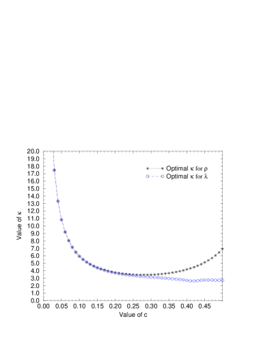
Figure 4: The optimal $\kappa$ values depending on $c$. For $c>0.2$, the optimal $\kappa$ is not the same for $\lambda(n)$ and $\rho(n)$.

Moreover, its largest and second-largest eigenvalues are both $1$, and slow convergence is unwanted in computer simulations. So we try to find other short-ranged actions for different pairs of $(c,\kappa)$. The short-range property of the action seems to depend largely on $\kappa$, so we optimize $\kappa$ for every value of $c$. The result is plotted in figure 4.

Up to the first half of the $c$-values, the optimized action remains fairly local. It is a smooth transition between the nearest-neighbor action $c=0$, $\kappa=\infty$, and the not very short ranged actions at $c>0.3$. Figure 5 shows the radius of $\rho(n)$ defined by

$$r_{\rho}^{2}=\frac{\sum_{n}|\rho(n)|n^{2}}{\sum_{n}|\rho(n)|}$$ (50)

Figure 5: The radius for the optimal $\kappa$ values depending on $c$.

For $c<0.3$ and the corresponding optimal $\kappa$ the value of $r_{\rho}$ is quite small. At small values of $c$, the next-to-leading eigenvalue is close to $1$, therefore it seems that the best choice is found in the middle of the possible $c$-values: For $c=0.25$ the action is still very local and it converges very fast. Additionally, it may be treated analytically. Actions with $c<0.25$ are a little bit more short-ranged, but their eigenvalue of convergence is larger and there are no nice analytic expressions for them.

4.4 Optimal action for 4$d$ including the mass

We assume that in $4d$ the situation is similar to the one dimensional case. The ’flat’ blocking seems to be one of the optimally short ranged actions, moreover it is treatable analytically much further than for other choices of $c_{i}$. The optimal $\kappa$ is $\kappa=3.3675$ for the massless action if we optimize for $r_{\rho}$. The value of $r_{\rho}$ stays at roughly $r_{\rho}=1.6$ for all masses where optimization is possible.

We may now extend the optimization to the massive actions. The parameter $\kappa$ may be optimized at each step on the renormalized trajectory. We first move into the Gaussian FP and then add a small mass, say $m=0.001$. Now at each blocking the value of $\kappa$ is optimized for locality. The result of the optimization is displayed below in figure 6.

Figure 6: The optimal values of $\kappa$ for mass values up to $m=2$. We see that the optimal $\kappa$ values would approach zero for masses larger than $m=3$. For $m>2$ an optimization by tuning $\kappa$ does not lead to a sufficiently short ranged action.

5 Conclusions

The convergence properties of a general RG transformation have been analized in this work. The observation is that the next-to-leading eigenvalue of the transformation can be in principle any number depending on the choice of the blocking function. This eigenvalue corresponds to a redundant operator, which does not produce lattice artifacts. The eigenvalues obtained by dimensional analysis are still present – they are responsible for the artifacts $a^{2n}$. We have shown that it is possible to optimize the parameters of the block transformation for locality and that ’flat’ blocking configurations where the fine lattice sites are weighted equally to obtain the coarse fields are preferred candidates for local actions.

A more detailed discussion can be found in [12]. I want to thank Ferenc Niedermayer for many useful discussions and Peter Hasenfratz for his support.

References

-
[1]
P. Hasenfratz and F. Niedermayer, Nucl. Phys. B 414, 785 (1994)
P. Hasenfratz Nucl. Phys. B Proc. Suppl. 34B, 3 (1994)
F. Niedermayer Nucl. Phys. B Proc. Suppl. 34B, 513 (1994) -
[2]
T. DeGrand, A .Hasenfratz, P. Hasenfratz and F. Niedermayer, Nucl. Phys. B 454, 587; ibid. 615 (1995)
F. Farchioni, P. Hasenfratz F. Niedermayer and A. Papa, Nucl. Phys. B 454, 638 (1995)
M. Blatter and F. Niedermayer, hep-lat 9605017 - [3] T. DeGrand, A .Hasenfratz, P. Hasenfratz, P. Kunszt and F. Niedermayer, hep-lat 9608056
- [4] L. P. Kadanoff, Physics 2, 263 (1966)
- [5] K. G. Wilson, Phys. Rev. D 10, 2445 (1974)
- [6] K. G. Wilson, Rev. Mod. Phys. 47, 773 (1975); 55, 583 (1983)
- [7] U-J. Wiese, Phys. Lett. B 315, 417 (1993)
- [8] W. Bietenholz, E. Focht and U-J. Wiese, hep-lat/940918
- [9] F. Niedermayer, hep-lat/9608097
- [10] T. L. Bell and K. G. Wilson, Phys. Rev. B 11, 3431 (1975)
- [11] W. Bietenholz, R. Brower, S. Chandrasekharan and U-J. Wiese, hep-lat/9612007
- [12] P. Kunszt, “Fixed Point Actions For Fermions”, PhD Thesis at the University of Berne.