FIXED POINT FOUR-FERMI THEORIES

I review dynamical chiral symmetry breaking in four-fermi models, including results of Monte Carlo simulations with dynamical fermions. For $2<d<4$, where the phase transition defines an ultraviolet fixed point of the renormalisation group, the continuum theory may either be describable using the large-$N_{f}$ expansion, as in the case of the Gross-Neveu model, or be intrinsically non-perturbative, as in the case of the Thirring model. For $d=4$, the models are trivial and are described by a mean field equation of state with logarithmic corrections to scaling, which may nonetheless define new universality classes distinct from those of ferromagnetism.

1 Introduction

In this talk I will review recent progress in our understanding of four-fermi theories, by which I mean quantum field theories described by the Lagrangian density

$${\cal L}=\bar{\psi}_{i}(\partial{\!\!\!/}\,+m)\psi_{i}\pm{{g^{2}}\over{2N_{f}}}(\bar{\psi}_{i}\Gamma\psi_{i})^{2}.$$ (1)

$\Gamma$ denotes a $4\times 4$ matrix constructed from Dirac $\gamma$-matrices, and the sign of the interaction is chosen so as to be attractive between fermion and anti-fermion. The index $i$ runs over $N_{f}$ distinct fermion flavors. I will discuss these models in spacetime dimension $2<d\leq 4$, paying most attention to the cases $d=3$ and $d=4$.

What are the motivations for studying such models? Their generic behaviour is that dynamical breaking of a chiral symmetry occurs at some strong value of the coupling $g^{2}$, where non-perturbative methods must be applied. In this talk I shall discuss and compare three such methods: the large-$N_{f}$ expansion, use of the Schwinger-Dyson equation, and lattice Monte Carlo simulation. Other methods, such as variational $\!{}^{{\bf?}}$ and derivative expansion $\!{}^{{\bf?}}$ approaches, have also been applied. The picture which is emerging is that the symmetry breaking transitions in these fermionic models define new universality classes, resembling qualitatively, but not quantitatively, those which apply to the study of ferromagnetic phase transitions.

Phenomenologically, four-fermi theories were of course originally introduced by Fermi to describe the weak interaction $\!{}^{{\bf?}}$, and were next applied to dynamical chiral symmetry breaking in the strong interaction by Nambu and Jona-Lasinio $\!{}^{{\bf?}}$. More recently they have appeared in discussions of dynamical mass generation in the Standard Model, in such scenarios as walking technicolor $\!{}^{{\bf?}}$, and the top-mode standard model in which the Higgs scalar is a $t\bar{t}$ bound state $\!{}^{{\bf?}}$. In three spacetime dimensions, there may be applications to high-$T_{c}$ superconductivity $\!{}^{{\bf?}}$, for instance in describing non-Fermi liquid behaviour in the normal phase $\!{}^{{\bf?}}$.

2 The Gross-Neveu Model for $d=3$

I will begin by discussing the simplest model, the Gross-Neveu (GN) model $\!{}^{{\bf?}}$, in which most of the important theoretical issues are already present. The Lagrangian is

$${\cal L}_{GN}=\bar{\psi}_{i}(\partial{\!\!\!/}\,+m)\psi_{i}-{{g^{2}}\over{2N_{f}}}(\bar{\psi}_{i}\psi_{i})^{2}.$$ (2)

For bare fermion mass $m=0$, there is a discrete chiral symmetry

$$\psi\mapsto\gamma_{5}\psi\;\;\;;\;\;\;\bar{\psi}\mapsto-\bar{\psi}\gamma_{5},$$ (3)

which is spontaneously broken whenever a non-vanishing condensate $\langle\bar{\psi}\psi\rangle$ is generated. To proceed, we introduce a bosonic scalar auxiliary field $\sigma$ and rewrite

$${\cal L}_{GN}=\bar{\psi}_{i}(\partial{\!\!\!/}\,+m+\sigma)\psi_{i}+{N_{f}\over{2g^{2}}}\sigma^{2}.$$ (4)

The original Lagrangian (2) can be recovered by Gaussian functional integration over $\sigma$. Chiral symmetry breaking for $m\to 0$ is now signalled by a non-vanishing vacuum expectation value $\Sigma\equiv\langle\sigma\rangle$ for the scalar field: it then follows from (4) that the fermion gets a dynamically generated mass $M\simeq\Sigma$.

We can calculate $\Sigma$ using an expansion in inverse powers of $N_{f}$, the number of flavors. This expansion associates a factor $N_{f}$ with each closed fermion loop, and in effect $1/\surd N_{f}$ with each fermion-scalar interaction vertex. To leading order, in the chiral limit $m\to 0$, only the tadpole diagram shown in Fig. 1a contributes to $\Sigma$, leading to the self-consistent Gap Equation:

$${\Sigma\over g^{2}}=\int_{p}\mbox{tr}{1\over{ip{\!\!\!/}\,+\Sigma}},$$ (5)

or, with a simple UV cutoff $\Lambda$ on momentum (note $2<d<4$)

$${1\over g^{2}}={8\over{(4\pi)^{d\over 2}(d-2)}}\left[{\Lambda^{d-2}\over{\Gamma({d\over 2})}}-\Sigma^{d-2}\Gamma(2-\textstyle{d\over 2})\right].$$ (6)

Figure 1: Leading order diagrams in the GN model

Equation (6), relating a bare coupling constant $g^{2}$ to both a UV scale $\Lambda$ and a physical scale $\Sigma$, can be interpreted as a renormalisation condition. It turns out to be the physical solution of (5) for couplings larger than the critical coupling $g_{c}^{2}$ given by

$${1\over g_{c}^{2}}={{8\Lambda^{d-2}}\over{(4\pi)^{d\over 2}(d-2)\Gamma({d\over 2})}},$$ (7)

at which point chiral symmetry is spontaneously broken (see Fig. 4). Only for $g^{2}\to g_{c}^{2}$, can the ratio $\Lambda/\Sigma$ be made to diverge, implying a continuum limit. Note that it is also possible to approach the continuum limit from the symmetric phase $\!{}^{{\bf?}}$.

Remarkably, for $2<d<4$, to the same leading order in $1/N_{f}$ all dependence on $\Lambda$ is absorbed in defining the value of $g_{c}^{2}$. The only other Green function involving a fermion loop is the scalar two-point function shown in Fig. 1b, but in the vicinity of the fixed point, once (6) is taken into account the scalar propagator is finite and can be expressed in closed form $\!{}^{{\bf?}}$. Eg, for $d=3$,

$$D_{\sigma}(k)={1\over N_{f}}{{2\pi\surd k^{2}}\over{(k^{2}+4\Sigma^{2})\tan^{-1}\left({{\surd{k^{2}}}\over{2\Sigma}}\right)}}.$$ (8)

In the large-$N_{f}$ limit $D_{\sigma}$ is essentially a chain of fermion bubbles. It is worth examining its behaviour in two limits. In the infra-red,

$${\lim_{k\to 0}}D_{\sigma}(k)\propto{1\over{k^{2}+4\Sigma^{2}}},$$ (9)

and hence the $\sigma$ resembles a fundamental boson with mass $2\Sigma$. This shows the scalar to be a weakly bound fermion - anti-fermion composite. In the ultra-violet, on the other hand, for general $d$ we have

$${\lim_{k\to\infty}}D_{\sigma}(k)\propto{1\over{k^{d-2}}}.$$ (10)

Thus the UV asymptotic behaviour is harder than that of a fundamental scalar, but still softer than the $1/k^{0}$ corresponding to a non-propagating auxiliary field. The strong interaction between fermion and anti-fermion is responsible for this modification, which in turn makes diagrams corresponding to higher order corrections, such as those of Fig. 2, less divergent than expected by naive power counting.

Figure 2: $O(1/N_{f})$ radiative corrections in the GN model

The result, known for a long time $\!{}^{{\bf?}}$, but discussed recently with renewed interest $\!{}^{{\bf?}}$, is that the $1/N_{f}$ expansion about the fixed point $g^{2}=g_{c}^{2}$ is exactly renormalisable for $2<d<4$.

An important aspect of the model’s renormalisability is that it depends on a precise cancellation between logarithmic divergences from different graphs $\!{}^{{\bf?}}$. This can be understood in terms of the four-fermi scattering amplitude, shown schematically in Fig. 3: there are three different types of logarithmic divergence, each represented by a blob, but in the massless limit only two tuneable parameters in the renormalised Lagrangian, implying a non-trivial consistency relation.

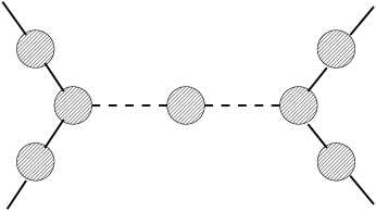
Figure 3: Renormalised four-fermi scattering amplitude

In turn this implies that in the deep UV limit the amplitude assumes a universal form

$${\lim_{k\to\infty}}{\cal M}_{ff\to ff}={A_{d}\over{N_{f}k^{d-2}}},$$ (11)

with the numerical constant $A_{d}=(4\pi)^{d\over 2}/4\Gamma(2-{d\over 2})B({d\over 2},{d\over 2}-1)$, and crucially no $1/N_{f}$ corrections. How then do higher order corrections manifest themselves? Fig. 4, showing a comparison between Monte Carlo data for $\Sigma$ from a $12^{3}$ lattice with the predictions of the leading order gap equation (5), gives a clue.

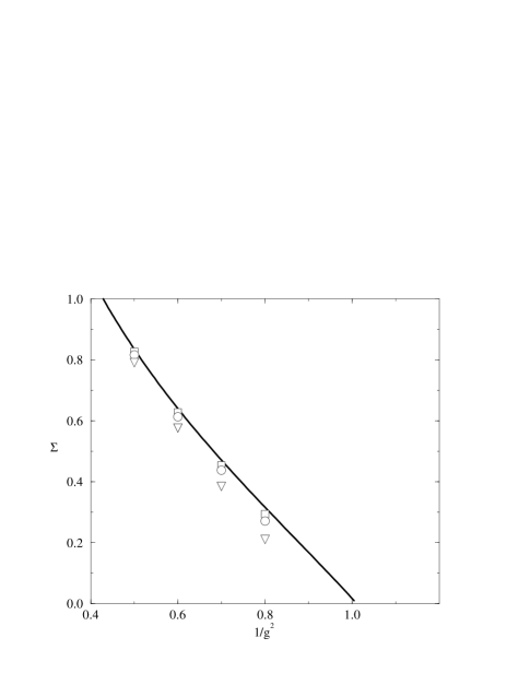
Figure 4: Plot of $\Sigma$ vs. $1/g^{2}$ for $N_{f}=24$ (squares), 12 (circles), and 6 (triangles). The line is the leading order gap equation prediction.

The corrections to $\Sigma$ are clearly $O(1/N_{f})$, suggesting that it is the behaviour of the bulk “thermodynamic” observables near the phase transition, in other words the IR physics, which most conveniently expresses the higher order information. If we define a reduced coupling

$$t={1\over g^{2}}-{1\over g_{c}^{2}},$$ (12)

then the scaling of the order parameter $\Sigma$ near the fixed point may be described by a set of critical exponents. Explicitly $\!{}^{{\bf?}}$ $\!{}^{{\bf?}}$:

$$\Sigma\propto t^{\beta} \beta={1\over{d-2}}+O\left({1\over N_{f}^{2}}\right);$$ with (13)

$$\Sigma|_{t=0}\propto m^{1\over\delta} \delta=(d-1)\left[1+{C_{d}\over N_{f}}\right];$$ with (14)

$$\chi\equiv{{\partial\Sigma}\over{\partial m}}\biggr{|}_{m=0}\propto|t|^{-\gamma} \gamma=1+{{d-1}\over{d-2}}{C_{d}\over N_{f}};$$ with (15)

$$M\propto|t|^{\nu} \nu={1\over{d-2}}\left[1+{{d-1}\over d}{C_{d}\over N_{f}}\right];$$ with (16)

$$D_{\sigma}(k)|_{t=0}\propto{1\over{k^{2-\eta}}} \eta=4-d-2{{d-1}\over d}{C_{d}\over N_{f}}.$$ with (17)

The numerical constant $C_{d}=1/B({d\over 2},2-{d\over 2})B({d\over 2},{d\over 2}-1)$. Several comments can be made:

1. The exponents obey certain consistency checks known as scaling and hyperscaling relations, eg.

   $$\gamma=\nu(2-\eta)\;\;\;;\;\;\;\beta={1\over 2}\nu(d-2+\eta).$$ (18)

   In statistical mechanics these are derived $\!{}^{{\bf?}}$ on the assumption that there is a single length scale characterising the important physics, namely the correlation length $\xi$. With $\xi\sim{\Lambda\over M}$, this is precisely the statement of renormalisability $\!{}^{{\bf?}}$.

2. In the limit $d\to 4$ the exponents assume their mean field (Landau-Ginzburg) values, namely

   $$\beta={1\over 2}\;\;;\;\;\delta=3\;\;;\;\;\gamma=1\;\;;\;\;\nu={1\over 2}\;\;;\;\;\eta=0.$$ (19)

3. The exponent $\eta$ is related to the anomalous scaling dimension $\gamma_{\bar{\psi}\psi}$ of the composite operator $\bar{\psi}\psi$ $\!{}^{{\bf?}}$:

   $$\eta=d-2\gamma_{\bar{\psi}\psi}.$$ (20)

   This implies for the scaling dimension $[\bar{\psi}\psi]$ the following:

   $$[\bar{\psi}\psi] = [\bar{\psi}\psi]_{0}-\gamma_{\bar{\psi}\psi}$$ (21)

   $$= d-1-(d-2+O(1/N_{f}))$$

   $$= 1+O(1/N_{f}).$$

   Hence the interaction term $(\bar{\psi}\psi)^{2}$ has scaling dimension $\simeq 2$, and is super-renormalisable, or in the renormalisation group (RG) sense relevant at the fixed point $\!{}^{{\bf?}}$. Note that the sign of the $O(1/N_{f})$ correction is not crucial to the argument $\!{}^{{\bf?}}$.

4. With the addition of $(\partial_{\mu}\sigma)^{2}$ and $\sigma^{4}$ terms, the model (4) becomes a Higgs-Yukawa (HY) theory, which is super-renormalisable for $d<4$. The UV fixed point of the GN model can thus be viewed as an IR fixed point of the HY model, at which the two extra operators become irrelevant $\!{}^{{\bf?}}$. This recalls the Wilson-Fisher fixed point in ferromagnetic models, and suggests an expansion in $\varepsilon=4-d$ as an alternative approach to the study of the universality class $\!{}^{{\bf?}}$. The equivalence of the two models in $d=3$ has been tested numerically $\!{}^{{\bf?}}$.

The final issue we should address for the GN model is the applicability of the $1/N_{f}$ expansion; in other words, for how small a value of $N_{f}$ may we trust its accuracy? Calculations of critical exponents are now available to $O(1/N_{f}^{2})$, and are compared to predictions from the $\varepsilon$-expansion of the HY model to $O(\varepsilon^{2})$, and the results of a $d=3$ Monte Carlo simulation for $N_{f}=2$ (the smallest value of $N_{f}$ that is simulable with a local lattice action using the staggered fermion formulation, which retains a chiral symmetry $\!{}^{{\bf?}}$) in Tab. 1.

Table 1: Critical exponents for the $d=3$ $N_{f}=2$ Gross-Neveu model

	large-$N_{f}$ $\!{}^{{\bf?}}$	$\varepsilon$-expansion $\!{}^{{\bf?}}$	Monte Carlo $\!{}^{{\bf?}}$
$\nu$	0.903	0.9480	1.00(4)
$\gamma/\nu$	1.2559	1.237	1.246(8)

The agreement is satisfactory, though it should be noted that the $1/N_{f}$ expansion for $\nu$, and the $\varepsilon$-expansion for $\gamma/\nu$ appear slowly if at all convergent, and the values quoted in the table have been obtained using resummation techniques $\!{}^{{\bf?}}$.

A similar comparison between the large-$N_{f}$ expansion to $O(1/N_{f}^{2})$ and Monte Carlo results has also been made for the GN model with continuous U(1) chiral symmetry, for $N_{f}=4$, with the results shown in Tab. 2.

Table 2: Critical exponents for the $d=3$ $N_{f}=4$ Gross-Neveu model with U(1) chiral symmetry

	large-$N_{f}$ $\!{}^{{\bf?}}$	Monte Carlo $\!{}^{{\bf?}}$
$\nu$	1.0(1)	1.02(8)
$\gamma/\nu$	1.055(13)	1.19(13)
$\beta/\nu$	0.973(6)	0.89(10)

In this case no resummation is attempted on the $1/N_{f}$ series: instead the quoted error reflects the size of the last term.

We conclude that the physical picture of dynamical symmetry breaking in the GN model given by the large-$N_{f}$ expansion is borne out by explicit simulations in $d=3$, and is qualitatively correct. Quantitative accuracy is limited by the apparently rather slow convergence of certain series, such as that for the exponent $\nu$.

3 The Thirring Model for $d=3$

The next model to consider, which will turn out to be more interesting, is the Thirring model, originally studied as a soluble model for $d=2$ and $N_{f}=1$ $\!{}^{{\bf?}}$, but here generalised. It differs from the GN model in that the contact interaction is between conserved currents:

$${\cal L}_{Thir} = \bar{\psi}_{i}(\partial{\!\!\!/}\,+m)\psi_{i}+{g^{2}\over{2N_{f}}}(\bar{\psi}_{i}\gamma_{\mu}\psi_{i})^{2}$$ (22)

$$= \bar{\psi}_{i}(\partial{\!\!\!/}\,+iA{\!\!\!/}\,+m)\psi_{i}+{N_{f}\over{2g^{2}}}A_{\mu}^{2},$$

where in the second line we have introduced an auxiliary vector field $A_{\mu}$. The form of the first term of (22) suggests that of an abelian gauge theory, except that the term quadratic in $A_{\mu}$ violates the gauge symmetry. In the chiral limit the Lagrangian (22) has a continuous U(1) chiral symmetry:

$$\psi\mapsto\exp(i\alpha\gamma_{5})\psi\;\;\;;\;\;\;\bar{\psi}\mapsto\bar{\psi}\exp(i\alpha\gamma_{5}).$$ (23)

It is possible to develop the $1/N_{f}$ expansion just as we did for the GN model, but this time in the chiral limit $\langle\bar{\psi}\psi\rangle$ remains zero to all orders, essentially because the trace over an odd number of $\gamma$-matrices vanishes. Consequently there is no fixed-point condition analogous to (6); however, provided a regularisation is specified which preserves current conservation $\partial_{\mu}(\bar{\psi}\gamma_{\mu}\psi)=0$, the auxiliary propagator $D_{\mu\nu}(k)$ is actually finite at leading order. For $d=3$ we have, explicitly

$${N_{f}\over g^{2}}D_{\mu\nu}(k)=\left(\delta_{\mu\nu}-{{k_{\mu}k_{\nu}}\over{k^{2}}}\right){1\over\displaystyle{1+{g^{2}\over{2\pi}}\left(m+{{k^{2}-4m^{2}}\over{2\surd k^{2}}}\tan^{-1}\left({{\surd k^{2}}\over{2m}}\right)\right)}}+{{k_{\mu}k_{\nu}}\over k^{2}}.$$ (24)

The longitudinal piece has no physical content, since it vanishes on being applied to a conserved current. As before, we can examine (24) in two opposite limits. In the UV, we find

$$\lim_{k\to\infty}D_{\mu\nu}(k)\propto\left(\delta_{\mu\nu}-{{k_{\mu}k_{\nu}}\over{k^{2}}}\right){1\over{k^{d-2}}}.$$ (25)

Once again, the modified asymptotic behaviour means that the divergence structure of higher order corrections is better behaved than expected: the Thirring model is thus exactly renormalisable for $2<d<4$ $\!{}^{{\bf?}}$ $\!{}^{{\bf?}}$ $\!{}^{{\bf?}}$. In the IR limit, the position of the pole in the transverse piece of $D_{\mu\nu}$ yields the mass $M_{V}$ of the propagating boson in the vector channel. For $d=3$ we have $\!{}^{{\bf?}}$

$$M_{V}=\cases{2m\left(1-2\exp\left(-{{2\pi}\over{mg^{2}}}\right)\right)&$mg^{2}\to 0$;\cr m\sqrt{{6\over{mg^{2}}}}&$mg^{2}\to\infty$.\cr}$$ (26)

The result depends in a non-trivial way on the dimensionless combination $mg^{2}$. In the weak coupling limit $mg^{2}\to 0$ the boson is a weakly bound fermion – anti-fermion state as in the GN model; however in the strong coupling limit its mass vanishes, yielding a model in which a massless vector mediates interactions between conserved currents. This is strongly suggestive that in this limit the Thirring model is identical to $\mbox{QED}_{3}$. Indeed, in general we expect the UV limit of the Thirring model to coinicide with the IR limit of $\mbox{QED}_{3}$, since in these limits the $1/N_{f}$ expansions of the two models coincide $\!{}^{{\bf?}}$ $\!{}^{{\bf?}}$.

We can summarise the distinct features of the Thirring model in $2<d<4$, as compared to the generic GN behaviour described in the previous section, with a number of equivalent statements:

1. There is no fixed-point condition.

2. The bare parameter $g^{2}$ is not renormalised.

3. The continuum theory contains a free dimensionless parameter $mg^{2}$.

4. The interaction $(\bar{\psi}\gamma_{\mu}\psi)^{2}$ is marginal in the RG sense.

Is this the whole story? All of these statements are made plausible in the context of the large-$N_{f}$ limit. We will now argue that the behaviour of the Thirring model is radically different for small $N_{f}$, if methods which are non-perturbative in $N_{f}$ are used.

The Schwinger-Dyson (SD) approach $\!{}^{{\bf?}}$ $\!{}^{{\bf?}}$ $\!{}^{{\bf?}}$ is to solve for the full inverse fermion propagator $S_{F}^{-1}=A(k)(ik{\!\!\!/}\,+M(k))$ self-consistently using integral equations, shown diagramatically in Fig. 5.

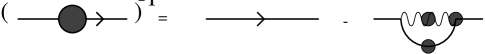
Figure 5: Schwinger-Dyson equation for the full fermion propagator

Any non-trivial solution $M(k)\not=0$ in the chiral limit signals dynamical mass generation. One analysis $\!{}^{{\bf?}}$ exploits a hidden local symmetry of (22) to fix a non-local “gauge” in which the wavefunction renormalisation $A(k)\equiv 1$. To proceed, the SD equations must be truncated; the full vector propagator is set to its large-$N_{f}$ form (24), and the full vertex $\Gamma_{\mu}(p,q)$ to the bare vertex $i\gamma_{\mu}$ – this second step is known as the ladder approximation, since in effect it ignores diagrams with crossed vector lines. With these approximations the SD equation may be solved in closed form in the strong coupling limit $g^{2}\to\infty$.

The result is that a non-trivial solution is found for small values of $N_{f}$; explicitly, for $d=3$

$${M\over\Lambda}\propto\exp\left(-{{2\pi}\over\sqrt{{N_{fc}\over N_{f}}-1}}\right)\;\;\Rightarrow\langle\bar{\psi}\psi\rangle|_{m=0}\propto\Lambda^{2}\exp\left(-{{3\pi}\over\sqrt{\textstyle{N_{fc}\over N_{f}}-1}}\right),$$ (27)

with $\Lambda$ a UV cutoff. The solution exists for

$$N_{f}<N_{fc}={{128}\over{3\pi^{2}}}\simeq 4.3.$$ (28)

If $N_{f}$ were a continuous parameter, then (27) would predict a UV fixed point as $N_{f}\to N_{fc}$. The essentially singular behaviour is similar to that of quenched $\mbox{QED}_{4}$ $\!{}^{{\bf?}}$; this type of transition has been given the label “conformal phase transition” $\!{}^{{\bf?}}$. How are we to interpret it in this case? It has been argued $\!{}^{{\bf?}}$ $\!{}^{{\bf?}}$ that for $g^{2}<\infty$ the critical curve $N_{fc}(g)$ is smooth. It is tempting to propose the phase diagram shown in Fig. 6, implying a sequence of fixed points $g^{2}_{c}(N_{f})$ for integer values of $N_{f}<N_{fc}$. The Thirring interaction $(\bar{\psi}\gamma_{\mu}\psi)^{2}$ has become relevant.

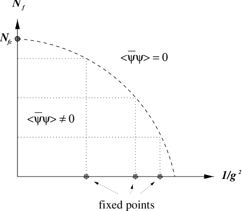
Figure 6: Proposed UV fixed points for the small-$N_{f}$ Thirring model

We should be cautious, however; a different sequence of truncations predicts $N_{fc}=\infty$ $\!{}^{{\bf?}}$. Indeed, the situation is reminiscent of $\mbox{QED}_{3}$, where chiral symmetry breaking is predicted for $N_{f}<N_{fc}$; the predicted value of $N_{fc}$ being highly sensitive to the assumptions used in solving the SD equation $\!{}^{{\bf?}}$ $\!{}^{{\bf?}}$. Once again, however, the same SD equation appears to describe both models, but in opposite momentum regimes, suggesting that their equivalence may hold beyond the large-$N_{f}$ approximation.

The UV behaviour of the Thirring model, if non-trivial, is genuinely non-perturbative, since there is no small dimensionless parameter in play at the putative fixed points. In this sense the Thirring model resembles the strong-coupling behaviour of $\mbox{QED}_{4}$ $\!{}^{{\bf?}}$ $\!{}^{{\bf?}}$, and hence is a suitable case for lattice Monte Carlo treatment. Indeed, to the best of my knowledge the three dimensional Thirring model may be the simplest fermionic model requiring a numerical solution, and thus deserves study by lattice theorists interested in simulating dynamical lattice fermions.

Lattice studies of the Thirring model have been made by two groups; I will briefly summarise our results $\!{}^{{\bf?}}$: details of the other group’s approach are given by the next speaker. $\!{}^{{\bf?}}$ The lattice formulations we have used differ in detail. I will suppress technical details, though it is still not clear how important they might turn out to be; one might hope that the number of distinct universality classes for fixed $N_{f}$ consistent with the breaking of the symmetry (23) is small. We have studied lattice models corresponding to $N_{f}=2$, 4 and 6 on volumes $8^{3}$, $12^{3}$ and $16^{3}$, with bare fermion masses $ma=0.05,\ldots,0.01$ ($a\sim\Lambda^{-1}$ is the lattice spacing).

First let’s discuss the evidence for spontaneous chiral symmetry breaking. We have measured $\Sigma=\langle\bar{\psi}\psi\rangle$ for various $m$ and $g^{2}$, and fitted our data to the equation of state (EOS)

$$m=A\left({1\over g^{2}}-{1\over g_{c}^{2}}\right)\Sigma+B\Sigma^{\delta}.$$ (29)

The exponent $\delta$ is identical to that of (14) – the form (29) makes the implicit assumption that $\delta-1/\beta=1$, which is consistent with the ladder approximation $\!{}^{{\bf?}}$. To explore (29), it is convenient to display the data in the form of a Fisher plot, ie., $\Sigma^{2}$ versus $m/\Sigma$. For the mean field exponents (19), this plot yields curves of constant $g^{2}$ as evenly spaced parallel straight lines, intercepting the vertical axis for $g^{2}>g_{c}^{2}$, the horizontal axis for $g^{2}<g_{c}^{2}$, and passing through the origin at the critical coupling. Any deviation signals a departure from the predictions of mean field theory. In Figs. 7, 8, and 9 we show Fisher plots respectively for $N_{f}=2$, 4 and 6.

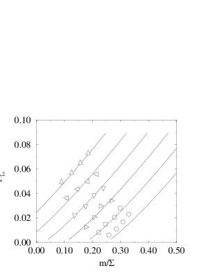
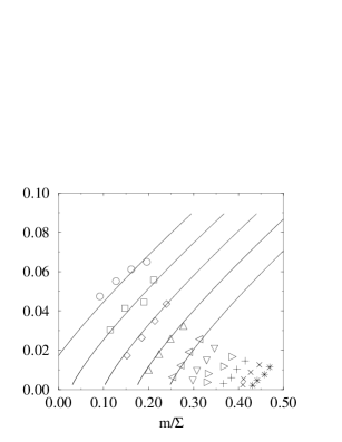
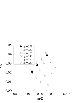
Figure 7:                                    Figure 8:

Figure 9:

The main features to note are that the $N_{f}=2,4$ data show different curvature, and that the $N_{f}=6$ data appear to be accumulating in the sub-critical region. The results of a fit to (29), which include a finite volume scaling analysis for $N_{f}=2$, are summarised in Tab. 3.

Table 3: Fits to the Equation of State

	$N_{f}=2$	$N_{f}=4$	$N_{f}=6$
$1/g_{c}^{2}$	1.92(2)	0.66(1)	no fit
$\delta$	2.75(9)	3.43(9)	found

We conclude that the $N_{f}=2$ and $N_{f}=4$ models do have fixed points, and that even if we relax the assumptions implied in (29) they fall in distinct universality classes; the data collected so far support $4<N_{fc}<6$,

Next consider susceptibilities, which are equivalent to spatially integrated two-point functions. By analogy with ferromagnetic models we define a “longitudinal” (ie. scalar) susceptibility $\chi_{l}$ and a “transverse” (ie. pseudoscalar) susceptibility $\chi_{t}$ as follows:

$$\chi_{l}=\sum_{x}\langle\bar{\psi}\psi(0)\bar{\psi}\psi(x)\rangle\;\;\;;\;\;\;\chi_{t}=\sum_{x}\langle\bar{\psi}\gamma_{5}\psi(0)\bar{\psi}\gamma_{5}\psi(x)\rangle.$$ (30)

The longitudinal susceptibility has contributions from diagrams with both connected ($\sqcap\!\!\!\!\sqcup$) and disconnected ($\circ$) fermion lines (ie. flavor non-singlet and singlet channels respectively), plotted in Fig. 10.

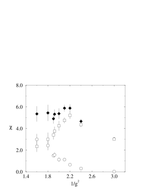
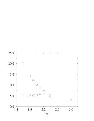
Figure 10:                                    Figure 11:

The relative importance of the disconnected piece, which is entirely due to sea quark loops, rises significantly in the broken symmetry phase. Fig. 11 shows that in the symmetric phase $\chi_{l}$ ($\circ$) and $\chi_{t}$ ($\sqcap\!\!\!\!\sqcup$) are approximately equal, as required by chiral symmetry, whereas in the broken phase $\chi_{t}\gg\chi_{l}$, since $\chi_{t}\propto M_{\pi}^{-2}$, and we expect the pion to be a Goldstone boson in the chiral limit. The ratio $\chi_{l}/\chi_{t}=R(m,g^{2})$ is another interesting quantity to examine. In general, for fixed $g^{2}$, $R$ varies strongly as a function of $m$ as $m\to 0$, tending in the chiral limit to zero in the broken phase and to a constant $\sim O(1)$ in the symmetric phase. Exactly at the critical coupling, however, it follows from the EOS (29) and the chiral Ward identity that $\!{}^{{\bf?}}$

$$R|_{g^{2}=g_{c}^{2}}={1\over\delta},$$ (31)

independently of $m$. Thus numerical measurements of $R$ give an independent estimate of the exponent $\delta$. In Fig. 12 we show data for $N_{f}=2$ in the vicinity of the critical coupling, for $1/g^{2}=1.9$ ($\circ$), 1.92 ($\sqcap\!\!\!\!\sqcup$), and 2.0 ($\diamond$), together with the value of ${1\over\delta}$ from Tab. 3.

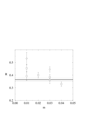
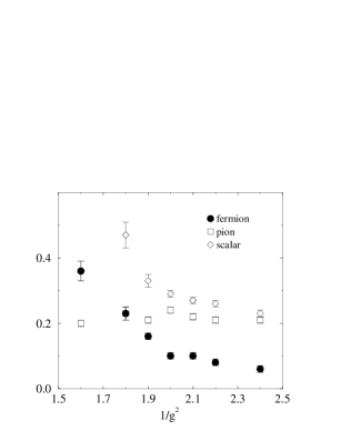
Figure 12:                                    Figure 13:

The data suggest that $R$ may become independent of $m$ at criticality once finite volume effects are taken into account $\!{}^{{\bf?}}$. Whilst this result is preliminary, it is interesting because measuring $R$ may be the most promising method of testing the equivalence of the Thirring model with $\mbox{QED}_{3}$ in future simulations.

Finally I present results on the mass spectrum for $N_{f}=2$, both for the physical fermion $f$ and for scalar and pseudoscalar $f\bar{f}$ bound states. A $16^{3}$ lattice is really too small in the timelike direction for any great precision; however Fig. 13 demonstrates that the level ordering of the states varies sharply across the transition. There is no evidence for the absence of light composite states in the symmetric phase, as predicted for the case of a conformal phase transition $\!{}^{{\bf?}}$. One further result is that in the vector channels in the symmetric phase there are light states in both “vector” ($\bar{\psi}\gamma_{\mu}\psi$) and “axial vector” ($\bar{\psi}\gamma_{\mu}\gamma_{5}\psi$) channels: the latter is not present in the large-$N_{f}$ approximation $\!{}^{{\bf?}}$.

So, the Thirring model is a good theoretical laboratory for non-perturbative dynamical symmetry breaking. In future studies it will be interesting to refine the spectroscopy, perhaps to explore the effects of a strongly-interacting continuum above the $f\bar{f}$ threshold. More effort is still needed to pin down the value of $N_{fc}$, and to see if the Thirring model and $\mbox{QED}_{3}$ are equivalent descriptions of the same critical dynamics.

4 The Nambu – Jona-Lasinio Model for $d=4$

After all these nice results, it is natural to demand what happens in the physical dimension $d=4$. Once again we revert to the GN model in the large-$N_{f}$ expansion. As $d\to 4$, the expansion loses the property of renormalisability, essentially because the “vacuum polarisation” contribution to the auxiliary two-point function gets a subleading $\ln\Lambda$ divergence. This must be compensated by the introduction of a kinetic term $(\partial_{\mu}\sigma)^{2}$ in the renormalised Lagrangian. If instead we choose to work with a finite cutoff $\Lambda$, then it is possible to make do without introducing the scalar kinetic term, at the cost of a residual logarithmic dependence on the UV scale. A moderate separation of UV and IR scales is possible – the model is thus an effective theory, making continuum-like predictions but with $O(\ln\Lambda)$ scaling violations. The UV scale can be interpreted as that at which new physical information, in the form of a more fundamental theory, must be supplied. The technical name for this scenario is triviality  – in the continuum limit $\Lambda\to\infty$ all interaction strengths vanish, as we shall see below. In RG language, for $d=4$ it is now the Gaussian fixed point which dominates the low-energy physics, and different models differ only by logarithmic corrections from free field theory.

The model we will consider in detail is the Nambu – Jona-Lasinio (NJL) model $\!{}^{{\bf?}}$:

$${\cal L}_{NJL}=\bar{\psi}_{ip}(\partial{\!\!\!/}\,+m)\psi_{ip}-{g^{2}\over{2N_{f}}}\left[(\bar{\psi}_{ip}\psi_{ip})^{2}-(\bar{\psi}_{ip}\gamma_{5}\vec{\tau}_{pq}\psi_{iq})^{2}\right],$$ (32)

where $p,q$ run over an internal isospace. In the chiral limit ${\cal L}_{NJL}$ has an $\mbox{SU(2)}_{L}\otimes\mbox{SU(2)}_{R}$ axial symmetry, which at strong coupling is dynamically broken to $\mbox{SU(2)}_{V}$ by the generation of a condensate $\langle\bar{\psi}\psi\rangle$. This is similar to the pattern of symmetry breaking in the Higgs sector of the Standard Model, and has led to suggestions that the physical Higgs is a $f\bar{f}$ composite $\!{}^{{\bf?}}$. The field theory conventionally used to describe the Higgs sector is, of course, the O(4) linear sigma model, describing elementary scalars with a four-point interaction. Both theories are trivial, and once the extra operators corresponding to scaling violations are taken into account, then each has equivalent predictive power for the Standard Model $\!{}^{{\bf?}}$. That said, it is interesting to ask whether there is a distinction between theories such as the sigma model in which triviality is manifested through elementary scalars, and theories like the NJL model in which fermions are elementary but scalars are composite.

One way of understanding the distinction is via the wavefunction renormalisation constant $Z$, defined as the coefficient of $1/k^{2}$ in the scalar propagator in the IR limit $k^{2}\to 0$. For the sigma model, $Z$ is perturbatively close to one, whereas for the NJL model in the large-$N_{f}$ expansion, for $d<4$ $Z\propto\Sigma^{4-d}$ (eg. (8)), and for $d=4$ $Z\propto 1/|\ln\Sigma|$. In either case $Z$ vanishes in the continuum limit $\Sigma\to 0$, with $\Sigma$ measured in cutoff units: this is the compositeness condition $\!{}^{{\bf?}}$. Another difference lies in the relative ordering of scales. The interaction strength in the scalar sector is expressed in terms of the pion decay constant $f_{\pi}$, which must be finite for interactions to occur. For the sigma model,

$${{f_{\pi}}\over\Sigma}\sim O(1),$$ (33)

however the ratio between the order parameter $\Sigma$ and the physical Higgs mass $M_{\sigma}$ is

$${\Sigma\over M_{\sigma}}\sim{1\over\sqrt{g_{R}}}\sim|\ln\Sigma|^{1\over 2},$$ (34)

where $g_{R}$ is the renormalised $\phi^{4}$ coupling constant, which vanishes logarithmically in the continuum limit. For the NJL model, on the other hand, to leading order in $1/N_{f}$ we have  $\!{}^{{\bf?}}$ $\!{}^{{\bf?}}$

$${f_{\pi}\over\Sigma}\sim|\ln\Sigma|^{1\over 2}\;\;\;;\;\;\;{\Sigma\over M_{\sigma}}\sim O(1).$$ (35)

All these predictions follow from the PCAC relation $Zf_{\pi}^{2}=\Sigma^{2}$. In both cases, triviality is realised by the divergence of $f_{\pi}$ in units of the physical scale $M_{\sigma}$ in the continuum limit:

$${f_{\pi}\over M_{\sigma}}\sim|\ln\Sigma|^{1\over 2}.$$ (36)

The different triviality scenarios also predict different forms for the equation of state. Recall that in $d=4$ the critical exponents take mean field values (19). Due to triviality the terms in the EOS (29) are modified by logarithmic corrections, to give the form

$$m=A\left({1\over g^{2}}-{1\over g_{c}^{2}}\right){\Sigma\over{|\ln\Sigma|^{q_{1}}}}+B{\Sigma^{3}\over{|\ln\Sigma|^{q_{2}}}}.$$ (37)

In the sigma model, the powers $q_{1}$ and $q_{2}$ can be found analytically by using the RG to evolve the coupling from a generic value into the perturbative regime $\!{}^{{\bf?}}$: this works because even the perturbative EOS predicts symmetry breaking. For the NJL model, by contrast, symmetry breaking only occurs for large coupling strengths, where the only guide is the large-$N_{f}$ approach $\!{}^{{\bf?}}$. The predictions are shown in Tab. 4 (the two RG values quoted for $q_{1}$ correspond to U(1) and SU(2) symmetries respectively).

Table 4: The correction exponents $q$ for $d=4$

	sigma	NJL	‘Thirring’ $\!{}^{{\bf?}}$	‘GN’ $\!{}^{{\bf?}}$
$q_{1}$	0.4, 0.5	0	0.36(11)	0.016(11)
$q_{2}$	1	$\!\!\!\!\!-1$	$\,\,\,0.485(17)$	$\!\!\!\!\!-0.553(18)$

Corrections to the mean field EOS have been analysed in several recent studies $\!{}^{{\bf?}}$ $\!{}^{{\bf?}}$ $\!{}^{{\bf?}}$, which use two different lattice implementations of the four-fermi interaction. The first, which in $d=3$ we have used to define the lattice GN model, formulates the auxiliary fields $\sigma$ on the sites of the dual lattice $\!{}^{{\bf?}}$, so that each $\bar{\psi}\psi$ pair interacts with all other sites sharing a hypercube. This has been used in a study of the $N_{f}=2$ NJL model with $\mbox{SU(2)}_{L}\otimes\mbox{SU(2)}_{R}$ symmetry $\!{}^{{\bf?}}$. The second, which in $d=3$ defines the lattice Thirring model, formulates the auxiliaries on the lattice links  $\!{}^{{\bf?}}$; the $N_{f}=4$ model with U(1) chiral symmetry was then studied $\!{}^{{\bf?}}$. The fitted values of the $q$ exponents are also given in Tab. 4. We should comment that logarithmic corrections are hard to isolate numerically, and that results are sensitive to assumptions about the size of the scaling region about the fixed point $\!{}^{{\bf?}}$. Nonetheless, the values found do suggest that the ‘GN’ and ‘Thirring’ formulations have qualitatively different scaling violations, the former resembling the large-$N_{f}$ predictions and the latter the sigma model. How stable the quoted $q$’s are, and whether the lattice-regularised models fall into distinct universality classes (the notion is still valid, since corrections to scaling can also be universal $\!{}^{{\bf?}}$), are issues for further study.

Further support for the distinct nature of models with composite scalars comes from a study of finite volume corrections when the ‘GN’ simulation is run directly in the chiral limit $m=0$ $\!{}^{{\bf?}}$. On a finite system in this limit the order parameter $\Sigma$ is strictly zero; we must instead monitor the quantity $|\Phi|$ defined by

$$|\Phi|=\biggl{\langle}\sqrt{{1\over 2}\mbox{tr}\bar{\Phi}^{\dagger}\bar{\Phi}}\biggr{\rangle}\;\;\;;\;\;\;\bar{\Phi}={1\over V}\sum_{x}\left(\sigma(x)+i\vec{\tau}.\vec{\pi}(x)\right),$$ (38)

where $\sigma,\vec{\pi}$ are the auxiliary fields. In Fig. 14 we plot $\Delta\equiv|\Phi|-\Sigma_{0}$ versus $1/g^{2}$, where $\Sigma_{0}$ is the order parameter from the EOS (37) extrapolated to the chiral limit. For a theory with fundamental

Figure 14: Finite volume correction for the NJL model. The vertical line shows the estimate for $1/g^{2}_{c}$.

scalars, the correction is predicted to be of the form $\!{}^{{\bf?}}$

$$\Delta\propto{1\over{L^{2}\Sigma_{0}}},$$ (39)

where $L$ is the linear size of the system ($L=16$ in this case). For a composite scalar, however, in the large-$N_{f}$ approximation the prediction becomes

$$\Delta\propto{1\over{L^{2}\Sigma_{0}|\ln\Sigma_{0}|}}.$$ (40)

As shown in the figure, (40) provides a much more convincing fit to the data.

5 Conclusions

To conclude, let me briefly summarise what each of the models we have looked at has taught us:

1. The Gross-Neveu models with discrete and continuous chiral symmetries in $d<4$ appear under good analytical and numerical control. They provide a paradigm for a non-perturbative fixed-point theory containing elementary fermion and composite scalar degrees of freedom, and a non-vanishing interaction at short distances. Two further applications of these models, which I have not had time to discuss, is that firstly unlike gauge theories they permit Monte Carlo simulation at non-vanishing chemical potential, and hence non-vanishing baryon number density. This has been applied in $d=3$ as a model effective theory of hadronic physics $\!{}^{{\bf?}}$. In $d=4$ simulations of QCD $\!{}^{{\bf?}}$ directly in the chiral limit are possible by including a gauge-invariant four-fermi interaction in the bare Lagrangian; the resulting model lies in the same universality class and hence contains the same IR physics as the true theory $\!{}^{{\bf?}}$.

2. The Thirring model in $d<4$ has a fixed point for small $N_{f}$ not described by the $1/N_{f}$ expansion. Genuine non-perturbative techniques need to be applied, and the model deserves to be used as a testbed for numerical lattice studies. The issue of its equivalence with $\mbox{QED}_{3}$ is intriguing and needs to be resolved.

3. There is lots more to learn about the nature of triviality in $d=4$. So far in looking at corrections to the equation of state we have pursued rather a “condensed matter” approach, and argued that composite models have a distinct form of scaling violation as compared to the standard ferromagnetic picture. It would be interesting to try to extract particle physics from these models, for instance, by asking whether they predict new triviality bounds on the Standard Model Higgs mass. Finally, there remains the fascinating possibility of actually finding new non-trivial fixed points in $d=4$ by expanding the space of couplings, say by introducing a gauge interaction such as in strongly-coupled QED $\!{}^{{\bf?}}$.

References

References

- [1] J.H. Yee, these proceedinngs.
- [2] K.-I. Aoki, proceedings of the International Workshop Perspectives of Strong Coupling Gauge Theories, Nagoya, Japan, 1996, ed. K. Yamawaki (World Scientific).
- [3] E. Fermi, Nuovo Cimento 11, 1 (1934), Z. Phys. 88, 161 (1934).
- [4] Y. Nambu and G. Jona-Lasinio, Phys. Rev. 122, 345 (1961).
- [5] B. Holdom, Phys. Lett. B 150, 301 (1985); K. Yamawaki, M. Bando and K. Matumoto, Phys. Rev. Lett. 56, 1335 (1986); T. Appelquist, D. Karabali and L.C.R. Wijewardhana, Phys. Rev. Lett. 57, 957 (1986).
- [6] Y.Nambu, in New Trends in Physics, proceedings of the XI International Symposium on Elementary Particle Physics, Kazimierz, Poland, 1988, eds. Z. Adjuk, S. Pokorski and A. Trautman (World Scientific, 1989); V.A. Miransky, M. Tanabashi and K. Yamawaki, Phys. Lett. B 221, 177 (1989), Mod. Phys. Lett. A 4, 1043 (1989); W.J. Marciano, Phys. Rev. Lett. 62, 2793 (1989); W.A. Bardeen, C.T. Hill and M. Lindner, Phys. Rev. D 41, 1647 (1990).
- [7] R. Shankar, Phys. Rev. Lett. 63, 203 (1989), Nucl. Phys. B 330, 433 (1990); N. Dorey and N.E. Mavromatos, Phys. Lett. B 250, 107 (1990), Nucl. Phys. B 386, 614 (1992).
- [8] I.J.R. Aitchison and N.E. Mavromatos, Phys. Rev. B 53, 9321 (1996).
- [9] D.J. Gross and A. Neveu, Phys. Rev. D 10, 3235 (1974).
- [10] Y. Kikukawa and K. Yamawaki, Phys. Lett. B 234, 497 (1990).
- [11] S.J. Hands, A. Kocić and J.B. Kogut, Phys. Lett. B 273, 111 (1991), Ann. Phys. 224, 29 (1993).
- [12] K.G. Wilson, Phys. Rev. D 7, 2911 (1974); D.J. Gross in Methods in Field Theory, Les Houches XXVIII, eds. R. Balian and J. Zinn-Justin (North Holland, 1976).
- [13] B. Rosenstein, B.J. Warr and S.H. Park, Phys. Rev. Lett. 62, 1433 (1989), Phys. Rep. 205, 59 (1991).
- [14] H.-J. He, Y.-P. Kuang, Q. Wang and Y.-I.Yi, Phys. Rev. D 45, 4610 (1992).
- [15] S.-K. Ma, Modern Theory of Critical Phenomena, (Benjamin, 1976).
- [16] G. Gat, A. Kovner and B. Rosenstein, Nucl. Phys. B 385, 76 (1992).
- [17] K.-I. Shizuya, Phys. Rev. D 21, 2327 (1980).
- [18] J. Zinn-Justin, Nucl. Phys. B 367, 105 (1991).
- [19] E. Focht, J. Jersák and J. Paul, Phys. Rev. D 53, 4616 (1996).
- [20] C.J. Burden and A.N. Burkitt, Europhys. Lett. 3, 545 (1987).
- [21] A. Coste and M. Lüscher, Nucl. Phys. B 323, 631 (1989).
- [22] J.A. Gracey, Int. J. Mod. Phys. A 6, 395 (1991), Int. J. Mod. Phys. A 9, 567 (1994).
- [23] L. Kärkkäinen, R. Lacaze, P. Lacock and B. Petersson, Nucl. Phys. B 415, 781 (1994), erratum Nucl. Phys. B 438, 650 (1995).
- [24] J.A. Gracey, Phys. Lett. B 308, 65 (1993), Phys. Rev. D 50, 2840 (1994).
- [25] W.E. Thirring, Ann. Phys. 3, 91 (1958); B. Klaiber, in Lectures in Theoretical Physics (Colorado 1967), eds. A.O. Barut and W. Brittin (Gordon and Breach, 1968).
- [26] G. Parisi, Nucl. Phys. B 100, 368 (1975); S. Hikami and T. Muta, Prog. Theor. Phys. 57, 785 (1977); Z. Yang, Texas preprint UTTG-40-90 (1990).
- [27] M. Gomes, R.S. Mendes, R.F. Ribeiro and A.J. da Silva, Phys. Rev. D 43, 3516 (1991).
- [28] S.J. Hands, Phys. Rev. D 51, 5816 (1995).
- [29] D. Espriu, A. Palanques-Mestre, P. Pascual and R. Tarrach, Z. Phys. C 13, 153 (1982); A. Palanques-Mestre and P. Pascual, Comm. Math. Phys. 95, 277 (1984).
- [30] T. Itoh, Y. Kim, M. Sugiura and K. Yamawaki, Prog. Theor. Phys. 93, 417 (1995); M. Sugiura, Prog. Theor. Phys. 97, 311 (1997).
- [31] D.K. Hong and S.H. Park, Phys. Rev. D 49, 5507 (1994).
- [32] P.I. Fomin, V.P. Gusynin, V.A. Miransky and Yu. A. Sitenko, Riv. Nuovo Cimento 6, 1 (1983); V.A. Miransky, Nuovo Cimento A 90, 149 (1985).
- [33] V.A. Miransky and K. Yamawaki, Phys. Rev. D 55, 5051 (1997).
- [34] K.-I. Kondo, Nucl. Phys. B 450, 251 (1995).
- [35] R.D. Pisarski, Phys. Rev. D 29, 2423 (1984); T.W. Appelquist, M.J. Bowick, D. Karabali and L.C.R. Wijewardhana, Phys. Rev. D 33, 3704 (1986), ibid. 3774; M.R. Pennington and D. Walsh, Phys. Lett. B 253, 246 (1991); P. Maris, Phys. Rev. D 54, 4049 (1996).
- [36] J.B. Kogut, E. Dagotto and A. Kocić, Phys. Rev. Lett. 60, 772 (1988), Nucl. Phys. B 317, 253 (1989), ibid. 271; M. Göckeler, R. Horsley, P.E.L. Rakow, G. Schierholz and R. Sommer, Nucl. Phys. B 371, 713 (1992).
- [37] A. Kocić, J.B. Kogut and K.C. Wang, Nucl. Phys. B 398, 405 (1993).
- [38] L. Del Debbio and S.J. Hands, Phys. Lett. B 373, 171 (1996); L. Del Debbio, S.J. Hands and J.C. Mehegan, hep-lat/9701016 (1997)
- [39] S. Kim and Y. Kim, hep-lat/9605021 (1996); S. Kim, these proceedings.
- [40] A. Hasenfratz, P. Hasenfratz, K. Jansen, J. Kuti and Y. Shen, Nucl. Phys. B 365, 79 (1991).
- [41] A. Kocić and J.B. Kogut, Nucl. Phys. B 422, 593 (1994).
- [42] S.J. Hands and J.B. Kogut, hep-lat/9705015 (1997).
- [43] E. Brézin, J.C. Le Guillou and J. Zinn-Justin, in Phase Transitions and Critical Phenomena vol 6, eds. C. Domb and M. Green (Academic Press, 1976); J. Zinn-Justin, Quantum Field Theory and Critical Phenomena (Oxford Science Publications, 1989).
- [44] S.Kim, A. Kocić and J.B. Kogut, Nucl. Phys. B 429, 407 (1994).
- [45] A. Ali-Khan, M. Göckeler, R. Horsley, P.E.L. Rakow, G. Schierholz and H. Stüben, Phys. Rev. D 51, 3751 (1995).
- [46] Y. Cohen, S. Elitzur and E. Rabinovici, Nucl. Phys. B 220, 102 (1983).
- [47] S.P. Booth, R.D. Kenway and B.J. Pendleton, Phys. Lett. B 228, 115 (1989).
- [48] M. Göckeler, H.A. Kastrup, T. Neuhaus and F. Zimmermann, Nucl. Phys. B 404, 517 (1993).
- [49] B. Rosenstein, B.J. Warr and S.H. Park, Phys. Rev. D 39, 3088 (1989); S.J. Hands, A. Kocić and J.B. Kogut, Nucl. Phys. B 390, 355 (1993); S.J. Hands, S. Kim and J.B. Kogut, Nucl. Phys. B 442, 364 (1995).
- [50] J.B. Kogut and D.K. Sinclair, Nucl. Phys. B (Proc. Suppl.) 53, 272 (1997); I.M. Barbour, S.E. Morrison and J.B. Kogut, hep-lat/9612012 (1996).
- [51] R.C. Brower, Y. Shen and C.-I. Tan, Nucl. Phys. B (Proc. Suppl.) 34, 210 (1994); R.C. Brower, K. Originos and C.-I. Tan, Nucl. Phys. B (Proc. Suppl.) 42, 42 (1995).