EPHOU-97-006

NBI-HE-97-19

TIT/HEP–371

June 1997

Abstract

We study the fractal structure of space-time of two-dimensional quantum gravity coupled to $c=-2$ conformal matter by means of computer simulations. We find that the intrinsic Hausdorff dimension $d_{H}=3.58\pm 0.04$. This result supports the conjecture $d_{H}=-2\alpha_{1}/\alpha_{-1}$, where $\alpha_{n}$ is the gravitational dressing exponent of a spinless primary field of conformal weight $(n+1,n+1)$, and it disfavours the alternative prediction $d_{H}=2/|\gamma|$. On the other hand $\langle l^{n}\rangle\sim r^{2n}$ for $n>1$ with good accuracy, i.e. the the boundary length $l$ has an anomalous dimension relative to the area of the surface.

1 Introduction

We still do not understand the theory of quantum gravity. In four dimensions it has been difficult to reconcile quantum theory and gravity. We have been more successful in two dimensions. Matrix models [1, 2, 3] and Liouville field [4, 5] theory allow us to understand a lot about the interplay between two-dimensional quantum gravity and conformal field theory.

It is sometimes said the two-dimensional quantum gravity will tell us little about four-dimensional quantum gravity since there are no gravitons in two dimensions. However, many of the conceptional problems of a theory of quantum gravity remain the same in two and four dimensions. In a certain way two-dimensional quantum gravity is as “quantum like” as a theory can be: In the path integral we perform a summation of all geometries with weight one. This means that there is no classical background space-time around which we expand and our understanding of space-time in such a quantum world could indeed contain very important messages of use in higher dimensions.

From this point of view it is somewhat annoying that precisely the structure of space-time is the least understood in two-dimensional quantum gravity. The recent introduction of the so-called transfer matrix [6] allows us to analyse in a satisfactory way the fractal structure of space-time for pure two-dimensional quantum gravity [6, 7, 8] and it highlights the fact that the dimension of space-time in quantum gravity is a dynamical quantity. Even if our underlying theory is two-dimensional we cannot be sure that this is the case for the quantum average. In fact, the fractal dimension of pure two-dimensional quantum gravity is four !

While the transfer matrix technique works perfectly for pure two-dimensional quantum gravity it is difficult to implement in the case of where matter fields are coupled to two-dimensional gravity. The reason is simple: when performing the sum over intermediate states, we should not only sum over all geometries of a certain kind but also over intermediate states of the matter fields. This has until now been impossible and another strategy has been followed: the concept of intermediate states is redefined in such a way that the summation can be performed [9]. The price paid is that the concept of intermediate state looses its direct link to the geometry present at the underlying manifold. To be more specific, let us consider two-dimensional quantum gravity coupled to a $c=1/2$ conformal field theory. At a constructive level, this theory is realized as the theory of dynamical triangulations with Ising spins placed at the centers of the triangles and the coupling of the Ising spins at a certain critical value. The geometry is now well defined via the dynamical triangulations and we can discuss the propagation of a one-dimensional universe with length $\ell_{1}$ to another one-dimensional universe with length $\ell_{2}$, the two separated a geodesic distance $D$. In the case of pure gravity this problem is solved by the transfer matrix method which reduces the calculation to a summation over successive amplitudes between universes where the one-dimensional boundaries are separated an infinitesimal distance. The only technical problem in the case of pure gravity is that the summation over all intermediate length $\ell$ of the boundaries has to be performed. This problem was solved in [6]. When we have Ising spins at the centers of the triangles we have in addition to sum over possible spin assignments at the boundaries of length $\ell$. Presently this cannot be done analytically. This problem can be avoided by redefining what is meant by the distance relating two one-dimensional loops by only considering deformations from loops with all spin aligned to other loops where all spin are aligned (the prescription can be made precise). However, such loops might not have a well defined geodesic distance. Nevertheless, consistent scaling relations can be defined in terms of this modified distance. If we assume that the modified distance is proportional to the real geodesic distance when the quantum average is performed, we get the prediction that the fractal dimension of space-time for two-dimensional quantum gravity coupled to a conformal field theory of central charge $c$ is

$$d_{H}=\frac{2}{|\gamma(c)|},$$ (1)

where the string susceptibility is given by

$$\gamma(c)=\frac{c-1-\sqrt{(25-c)(1-c)}}{12}\,.$$ (2)

In particular, for an $(m,m\!+\!1)$ conformal field theory one obtains $d_{H}=2m$, and for the Ising model, which corresponds to $m=3$, one gets $d_{H}=6$. On the other hand, for $c=-2$ (a non-unitary conformal theory) we get

$$d_{H}(c=-2)=2,$$ (3)

i.e. the fractal dimension $d_{H}$ is equal to the dimension of the underlying manifold.

An alternative prediction of $d_{H}$ is obtained by use of the diffusion equation in Liouville theory [19]:

$$d_{H}=-2\frac{\alpha_{1}}{\alpha_{-1}}=2\times\frac{\sqrt{25-c}+\sqrt{49-c}}{\sqrt{25-c}+\sqrt{1-c}}\,.$$ (4)

The origin of this equation is to be found in the analysis of the diffusion equation in Liouville theory [19] and is based on the observation that for random walks on a two-dimensional manifolds of area $A$ we expect

$${\rm dim}[\,\left\langle r^{2}(t)\right\rangle_{A}\,]={\rm dim}[\,A^{2/d_{H}}\,]\,,$$ (5)

where $r(t)$ is the geodesic distance of the random walk at the (fictitious) diffusion time $t$ and the average refers to the functional integral over geometries and matter. In Liouville theory one can use the De-Witt short distance expansion of the heat kernel in terms of geodesic distance to deduce [19] that

$${\rm dim}[\,\left\langle r^{2}(t)\right\rangle_{A}\,]={\rm dim}[\,A^{-(\alpha_{-1}/\alpha_{1})}\,].$$ (6)

In eq. (6) $\alpha_{-n}$ denotes the gravitational dressing of an $(n\!+\!1,n\!+\!1)$ primary spinless conformal field, i.e.

$$\int\!d^{2}\xi\sqrt{g}\Phi_{n+1}(g)\to\int\!d^{2}\xi\sqrt{\hat{g}}\;e^{\alpha_{-n}\phi}\Phi_{n+1}(\hat{g})~{}~{}~{}{\rm for}~{}~{}~{}g_{\mu\nu}(\xi)=e^{\phi(\xi)}\hat{g}_{\mu\nu}(\xi),$$

where $\hat{g}_{\mu\nu}(\xi)$ is the background metric and $\Phi_{n}(g)$ satisfies $\Phi_{n}(e^{\phi}\hat{g})=e^{-n\phi}\Phi_{n}(\hat{g})$. The requirement that $e^{\alpha_{-n}\phi}\Phi_{n+1}(\hat{g})$ is a $(1,1)$ conformal field fixes

$$\alpha_{n}=\frac{2n}{1+\sqrt{(25-c-24n)/(25-c)}}\,.$$ (7)

It is an important assumption in this derivation that it is legal to commute the asymptotic De-Witt expansion of the heat kernel and the functional integral over geometry and matter. For $c=0$ one obtains $d_{H}=4$, in agreement with the transfer matrix prediction, while for $c=1/2$ (corresponding to the critical Ising model coupled to gravity in the transfer matrix formulation) one obtains $d_{H}=(\sqrt{97}+7)/4=4.212\ldots$. For $c=-2$ one obtains

$$d_{H}(c=-2)=\frac{3+\sqrt{17}}{2}=3.561\ldots\,.$$ (8)

Except for pure gravity the two predictions disagree. It is the purpose of the present work to test if any of the two predictions is consistent with numerical simulations. The available analytical methods have build-in assumptions. No assumptions have to be made by a brûte force numerical simulation of the system. Of course numerical methods have other problems, most notably that of accuracy. Until now the numerical simulations have been concentrated on systems with $c>0$, mainly the Ising spin coupled to gravity ($c=1/2$) and the three-state Potts model coupled to gravity ($c=4/5$) [10, 11, 12, 13]. The results have so far not been able to support the prediction (1) (i.e. $d_{H}=6$ and 10 for the Ising and the three-state Potts model, respectively). However, it could be argued that these dimensions are so large that it would be very difficult to observe them in numerical simulations with the present size of lattices. It is natural to require that one should be able to probe lattice distances $r$ such that

$$1\ll r\ll N^{1/d_{H}},$$ (9)

where $N$ is the number of triangles or vertices in the triangulation. For systems with $N<10^{6}$ it is clearly problematic to fulfill (9). It is however possible to measure the critical indices of Ising and three-state Potts models coupled to quantum gravity with good precision [14]. Since many of these critical indices come from integrated two-point functions which also measure $d_{H}$ it is not easy to understand how the critical properties come out right if (9) is never satisfied. Moreover, it was recently found that correlation functions defined in terms of geodesic distance scale consistently with the theoretical critical indices if and only if $d_{H}\approx 4$ [10, 12, 13]. These are indirect arguments in disfavour of (1), but of course not conclusive since numerical peculiarities could conspire and still allow us to determine the critical exponents without (9) ever being fulfilled. However, in order to avoid this discussion completely it is convenient to turn to the $c=-2$ system. This system is in a way the simplest coupled gravity-matter system. Within the context of dynamical triangulations it was the first system which could be explicitly solved [3], apart from pure gravity itself. Quite recently it has been possible to construct explicitly the two-point function using the transfer matrix methods [15] and thereby generalising the results known for pure gravity [7].

The advantage of the choice $c=-2$ is two-fold. The prediction from the transfer matrix formulation is $d_{H}=2$, while it from Liouville diffusion is 3.562 (see (3) and (8)). These values for $d_{H}$ are so small that one has no problem satisfying (9) for the sizes of systems available on the computer. Further, $c=-2$ is special since one does not have to perform Monte Carlo simulations in order to generate lattice configurations with the correct weight [16]. As we will review below there exists a recursive and very fast algorithm which allows us to generate directly independent triangulations. In this way one can use larger systems and obtain better statistics. This method was first used in [16] to investigate the fractal properties of space–time for the $c=-2$ system coupled to gravity. It was the first numerical confirmation of the fractal structure of quantum gravity in two dimensions. In this work the emphasis was put on the use of very large systems in order to get an unambiguous identification of continuum observables. Since then it has been shown that (a): finite size scaling is by far the most powerful tool for extracting critical properties in two-dimensional quantum gravity (i.e. the situation is similar to the one for ordinary statistical systems) and (b): the fractal properties of space-time have an interpretation as critical indices associated with two-point correlators, precisely as in ordinary statistical field theory [7, 11]. In this article we will show that (a) and (b) together with the powerful technique of recursive sampling available for $c=-2$ coupled to quantum gravity makes it possible to determine $d_{H}$ with a precision not known before.

The rest of this paper is organised as follows: In section 2 we discuss the model as well as the observables and their scaling. Section 3 outlines the numerical methods used. Section 4 contains a summary of the numerical results obtained, while section 5 estimates the finite size shift of geodesic distance from the theoretical point of view. In section 6 we discuss the results and the implications.

The results strongly support (8), i.e. it lends support to the prediction (4). However, we also find a surprising new scaling law for the boundaries in two-dimensional quantum gravity. A short report of some of the results discussed in this paper has appeared in [17].

2 The model

2.1 The partition function

Within the framework of dynamical triangulations the conformal theory of $c$ Gaussian fields $x^{\mu}$ coupled to quantum gravity is described by the following partition function

$$Z_{N}=\sum_{T_{N}\in{\cal T}_{N}}\frac{1}{{\cal S}_{T_{N}}}\int\prod_{i=1}^{N}dx_{i}\;\exp\frac{1}{2}\Bigl{(}\sum_{(ij)}(x_{i}-x_{j})^{2}\Bigr{)}\;\delta\Bigl{(}\sum_{i}x_{i}\Bigr{)},$$ (10)

where ${\cal T}_{N}$ denotes the set of triangulations of fixed topology (which we always assume is spherical) constructed from $N$ triangles. ${{\cal S}_{T_{N}}}$ is a symmetry factor. The $c$ independent Gaussian variables $x^{\mu}_{i}$ can be viewed as placed at the center of triangle $i$. They interact with the Gaussian variables at the neighbouring triangles and $\sum_{(ij)}$ denotes the sum over all such pairs of triangles.

The Gaussian integration can be performed and one obtains (up to a constant of proportionality)

$$Z_{N}=\sum_{T_{N}}\frac{1}{{\cal S}_{T_{N}}}\left(\det{}^{\prime}C_{T_{N}}\right)^{-c/2}\,,$$ (11)

where $C_{T_{N}}$ is the so-called adjacency matrix of the closed $\phi^{3}$-graph $\phi^{3}(T_{N})$ dual to $T_{N}$. From graph theory it is known that $\det^{\prime}\!C_{T_{N}}$ is equal to the number of rooted spanning trees in the graph $\phi^{3}(T_{N})$. Eq. (11) serves as a definition of a model when $c$ is not a positive integer, in particular when $c=-2$. The string susceptibility can be calculated in this model and it agrees with the continuum calculation in Liouville theory for a $c=-2$ theory.

It is seen that Eq. (11) is special if $c=-2$ since in this case we can use the fact that $\det^{\prime}\!C_{T_{N}}$ is the number of spanning trees of $\phi^{3}(T_{N})$, i.e. the number of possible ways to cut the $\phi^{3}(T_{N})$ graphs of spherical topology into tree diagrams. The triangulations in ${\cal T}_{N}$ are in one-to-one correspondence with the $\phi^{3}(T_{N})$ connected planar graphs with $N$ vertices and no external legs. This can be symbolically written as follows:

$$Z_{N}=\sum_{T_{N}}\frac{1}{{\cal S}_{T_{N}}}\!\sum_{\stackrel{{\scriptstyle\hbox{\scriptsize spanning trees}}}{{\hbox{\scriptsize in $\phi^{3}(T_{N})$}}}}1.$$ (12)

2.2 Trees and rainbows

Let us briefly describe the combinatorics associated with the decomposition of the planar graphs $\phi^{3}(T_{N})$ of spherical topology into trees and rainbow diagrams. Let $T_{n}$ and $R_{n}$ be the number of rooted dual tree diagrams with $n+1$ external legs and the number of rainbow diagrams with $n$ lines, respectively. Especially, we have $T_{1}=R_{0}=1$. Here, we mark one of the legs for each tree diagram and for each rainbow diagram in order to break the symmetry. Since any planar closed $\phi^{3}$ graph can be obtained from a spanning tree by connecting the external vertices of the tree by rainbow diagrams we can write (12) as [3] (See fig. 1)

$$Z_{N}=\frac{1}{3N}\!\sum_{\stackrel{{\scriptstyle\hbox{\scriptsize$k,l,m\geq 1$}}}{{\hbox{\scriptsize with $k+l+m=N+2$}}}}\!T_{k}T_{l}T_{m}R_{(N+2)/2}\,.$$ (13)

Figure 1: Partition function described by tree and rainbow diagrams.

To calculate $T_{n}$ and $R_{n}$ is easily done as follows. The tree diagrams satisfy the graphical Schwinger–Dyson equation shown in fig. 2a, i.e. $T_{n}$ satisfies

$$T_{n}=\sum_{k=1}^{n-1}T_{k}T_{n-k}\,.$$ (14)

In the same way the rainbow diagrams satisfy the graphical Schwinger–Dyson equation of fig. 2b, leading to an identical equation

Figure 2: Graphical representation of Schwinger–Dyson equations for (a) tree diagrams, (b) rainbow diagrams.

$$R_{n}=\sum_{k=0}^{n-1}R_{k}R_{n-k-1}\,.$$ (15)

In order to solve the Eqs. (14) and (15), we introduce the generating functions for the tree diagrams and the rainbow ones as

$$T(z)=\sum_{n=1}^{\infty}T_{n}z^{n-1},~{}~{}~{}~{}~{}~{}R(z)=\sum_{n=0}^{\infty}R_{n}z^{n}.$$ (16)

Then, Eqs. (14) and (15) are written by using the generating functions as

$$T(z)=1+zT(z)^{2},~{}~{}~{}~{}(T(0)=1),$$ (17)

$$R(z)=1+zR(z)^{2},~{}~{}~{}~{}(R(0)=1).$$

The solutions of (17) are

$$T(z)=R(z)=\frac{1}{2z}\Bigl{(}1-\sqrt{1-4z}\Bigr{)}.$$ (18)

Therefore, one finds

$$T_{n}=R_{n-1}=\frac{(2n-2)!}{n!(n-1)!}\,.$$ (19)

Using the relation (14), the partition function (13) finally can be written as a simpler expression,

$$Z_{N}=\frac{1}{N+2}T_{N+1}R_{(N+2)/2}\,.$$ (20)

2.3 Observables

We define the fractal structure of quantum gravity in the following way. Let us fix the space-time volume $V$. The average volume $S_{V}(R)$ of a spherical shell of radius $R$ is then

$$S_{V}(R)=\frac{1}{Z(V)}\int_{V}\!{\cal D}[g]{\cal D}\phi\,{\mathrm{e}}^{-S}\!\int\!d^{2}\xi\sqrt{g}\;\delta(D_{g}(\xi,\xi_{0})-R),$$ (21)

where $Z(V)$ is the partition function of gravity coupled to matter, with space-time constrained to have volume $V$, $\int_{V}$ symbolises that the integration of metrics fulfilling the same constraint, $\xi_{0}$ denotes an arbitrary marked point and $D_{g}(\xi,\xi_{0})$ the geodesic distance from the marked point $\xi_{0}$ to $\xi$, measured with respect to the metric $g$. We define the fractal dimension (or intrinsic Hausdorff dimension) $d_{h}$ of the space-time by

$$S_{V}(R)\sim R^{d_{h}-1}~{}~{}~{}~{}\hbox{for \ $R\sim 0$}.$$ (22)

It is important to notice that the limit $R\to 0$ is taken after the functional average is performed. Had we taken the limit $R\to 0$ before the functional average we would of course have obtained the result “$d_{h}$”$=2$ since each manifold is two-dimensional. However, the limit $R\to 0$ does not commute with the functional integral. It turns out that no matter how small $R$ is there will always be numerous metrics (i.e. a set of metrics of non-zero measure with respect to ${\cal D}[g]$) with the property that geodesic spheres of radius $R$ consist of many connected components. For such geometries we cannot necessarily expect a growth as slow as $R$. The precise growth of $S_{V}(R)$ for small $R$ becomes a subtle question of entropy of different metrics and from this description it is obvious that the phrase “fractal dimension” is quite appropriate if $d_{h}>2$.

In the case of pure two-dimensional gravity it is a remarkable fact that one can calculate $S_{V}(R)$ analytically [7, 11] (it can be expressed in terms of certain generalised hypergeometric functions). One finds

$$S_{V}(R)=R^{3}f(R/V^{\frac{1}{4}}),$$ (23)

where $f(0)>0$ and $f(x)\sim e^{-x^{4/3}}$ for large $x$. It is seen that a dimensionless scaling variable $R/V^{1/4}$ appears. For a general model such a dimensionless scaling variable, $R/V^{1/d_{H}}$ will define another intrinsic Hausdorff dimension $d_{H}$. From (22) and (23) we deduce that $d_{h}=d_{H}=4$ in the case of pure gravity. For general model we can write (23) as

$$S_{V}(R)=V^{1-1/d_{H}}F_{1}(R/V^{1/d_{H}}),$$ (24)

where

$$F_{1}(x)\sim x^{d_{h}-1},~{}~{}~{}~{}x\ll 1,$$ (25)

and $F_{1}(x)$ goes to zero as $e^{-x^{d_{H}/(d_{H}-1)}}$ for $x$ going to infinity. Eq. (24) has the form of a typical finite size scaling relation and we expect it to be valid not only for pure gravity, but also for gravity coupled to matter. Since $S_{V}(R)$ is easily measured in numerical simulations we can use Eq. (24) and (25) to extract $d_{h}$ and $d_{H}$. Using (24) and (25), one finds

$$S_{V}(R)\sim V^{1-d_{h}/d_{H}}R^{d_{h}-1},~{}~{}~{}~{}R/V^{1/d_{H}}\ll 1.$$ (26)

If space–time for large $V$ has the same fractal properties at all scales, one expects

$$d_{h}=d_{H}.$$ (27)

However, in our numerical simulations we do not assume this property $d_{h}=d_{H}$. It is one of our purposes to check if eq. (27) is realized for the $c=-2$ model.

Let us briefly describe how the above continuum description translates to the framework of dynamical triangulations. To a triangulation $T_{N}$ we can unambiguously associate a piecewise linear manifold with a metric dictated by the length assignment $\varepsilon$ to each link. From a practical point of view we use instead a graph-theoretical distance between vertices, links or triangles. In the limit of very large triangulations we expect that the different distances when used in ensemble averages will be proportional to each other. To be specific we will in the following operate with a “link distance” and a “triangle distance”. The link distance between two vertices is defined as the shortest link-path between the two vertices, while the triangle distance between two triangles is defined as the shortest path along neighbouring triangles between the two triangles. In this way the triangle distance becomes the link distance in the dual $\phi^{3}$ graph.

In the following we will report on the measurement of quantities related to the fractal structure of quantum space-time: The total length $\left\langle l\right\rangle$ and the higher moments $\left\langle l^{n}\right\rangle$ of spherical shells of (geodesic) radius $r$, and the distribution function $\rho(r,l)$ which measures the (average) number of connected components of the shells of length $l$ and radius $r$.

More precisely, let us consider the class of triangulations ${\cal T}_{N}$ which are dual to the connected closed $\phi^{3}$-graphs. The number of triangles (or vertices in the $\phi^{3}$-graphs), $N$, plays the role of volume. If $\varepsilon$ denotes the link length of the triangles the relation to the continuum volume is $V\sim\varepsilon^{2}N$, and we want to take a limit where $V$ is fixed while $\varepsilon\to 0$ and $N$ to infinity. We consider a spherical ball of radius $r$ and its shell for a given triangulation $T_{N}$. The spherical ball consists of all vertices with link distance $r^{\prime}\leq r$ and the spherical shell consists of all vertices with link distance $r$, where the distance is measured from a given vertex $v_{0}$ which is considered as the center of the spherical ball. In the same way we can define the spherical shell in terms of triangle distance. We will use both definitions in the following and we expect that after taking the statistical average they will be proportional to each other and that they will not affect the universal properties of correlation functions [18]. The spherical shell in general consists of a number of connected components if we define a connected component of the shell of vertices as a maximal set of vertices in the shell where all vertices can be connected via links in the shell. If we take the average over all positions of $v_{0}$ and all triangulations $T_{N}$, we get a distribution $\rho_{N}(l,r)$ of the length $l$ (measured in link units) of the connected components of the spherical shells of radius $r$, i.e.

$$\left\langle l^{n}\right\rangle_{r,N}\equiv\sum_{l=1}^{\infty}l^{n}\rho_{N}(l,r)\,.$$ (28)

In particular we introduce the special notation $n_{N}(r)=\left\langle l\right\rangle_{r,N}$, and since $n_{N}(r)$ is the discretized version of $S_{V}(R)$ we expect the fractal dimension to be related to $n_{N}(r)$ by

$$n_{N}(r)\sim r^{d_{h}-1},~{}~{}~{}~{}~{}~{}~{}1\ll r\ll N^{1/d_{H}}\,.$$ (29)

According to the general scaling arguments mentioned above [7, 10, 11] we expect the following behaviour for $n_{N}(r)$:

$$n_{N}(r)\sim N^{1-1/d_{H}}F_{1}(x),~{}~{}~{}~{}~{}x=\frac{r}{N^{1/d_{H}}}\,,$$ (30)

and we expect $F_{1}(x)$ to behave as $x^{d_{h}-1}$ for small $x$ and to fall off rapidly when $x\gg 1$.

3 Numerical method

3.1 The recursive algorithm

The recursive algorithm takes advantage of the factorisation property of the partition function (see Eq. (13)) in order to construct a typical configuration of $c=-2$ gravity. One constructs a rooted $\phi^{3}$ tree with the correct probability and then connects the outer links of the tree with a rainbow diagram also constructed with the correct probability. According to Eq. (14) the branching probability to divide a rooted tree diagram with $n+1$ external legs into two different rooted tree diagrams with $k+1$ and $n-k+1$ (“1” counts the root) external legs is given by

$$w(n,k)=\frac{T_{k}T_{n-k}}{T_{n}}\,.$$ (31)

If we want to construct a surface with $N$ triangles ($N$ must be even) we need to construct a tree with $N+2$ external legs. In practice, we start from the root, which has a tree with $N+2$ external legs attached to it. Then we proceed with branching the root into two trees with $k+1$ and $N+2-k$ external legs (remember that we also count the root leg), where $k$ is computed from Eq. (31). At each step we assign the number of external legs of the tree attached to each link according to the same formula and we keep an ordered list of the external legs of the whole tree. We add one such link to the list whenever $k=1$.

Then we proceed to connect the external legs with a rainbow diagram. This is possible since the total probability is the product of the probability of constructing the rooted tree Eq. (31) and the probability of constructing the corresponding rainbow diagram. According to Eq. (15), the probability of splitting a rainbow diagram with $n$ lines into two rainbows with $k$ and $n-1-k$ lines is given by:

$$u(n,k)=\frac{R_{k}R_{n-k-1}}{R_{n}}=w(n+1,k+1)\,,$$ (32)

since $R_{n-1}=T_{n}$. In practice we start from the root leg of the tree diagram and we split the rainbow containing $N/2+1$ lines into two parts containing $k$ and $N/2-k$ lines. Then we can connect the root leg with the appropriate member of the list containing the external legs of the tree mentioned above and proceed accordingly until we connect all external legs.

3.2 The simulations

The simulations are performed by generating a number of statistically independent configurations using the algorithm mentioned above. We use the high quality random number generator RANLUX [28, 29] whose excellent statistical properties are due to its close relation to the Kolmogorov K-system originally proposed by Savvidy et.al. [26, 27] in 1986. We centered our effort for good statistics on system sizes ranging from $2000$–$256000$ triangles. The number of configurations obtained depends on the lattice size and on the observable that we measure. We choose $20$ random vertices/triangles on each configuration in order to perform correlation function measurements. We need to collect more statistics to test Eq. (30), where we have between $4.2\times 10^{6}$ and $1.6\times 10^{6}$ configurations. For the $128K$ and $256K$ lattices we have $6\times 10^{5}$ and $2\times 10^{5}$ configurations respectively. It was possible to extract useful information about the short distance behaviour of the two point function $n_{N}(r)$ by generating a smaller number of configurations for system sizes having $512000$–$8192000$ triangles. We got $10000$ configurations for $N=512000$ and $1024000$, $4000$ for $N=2048000$ and $386$ for $N=8192000$ and we measured $n_{N}(r)$ by choosing many more initial random triangles/vertices. It is not possible to extract $d_{H}$ by using finite size scaling with so low statistics.

In order to measure the moments $\left\langle l^{n}\right\rangle_{r,N}$ and their scaling properties we need a factor of $10^{2}$ less configurations: We have approximately $50000$ configurations for each lattice size. Unfortunately, the computer effort for making the measurements is comparable to the one needed to test Eq. (30) with enough accuracy.

One subtle point in the simulations is the computation of the branching numbers given by Eqs. (31) and (32). Given the number $n$ we need to compute $k$. We do this by choosing a random number $r$ in the interval $[0,1)$. Then, e.g. for the case of trees, we compute

$$W(n,k)=\sum_{i=1}^{k}w(n,i)\,,$$ (33)

and we choose $k$ to be the integer such that $W(n,k)\geq r$. Using the symmetry of $w(n,k)$ around $n/2$ we can substantially reduce the computation time. Moreover $w(n,k)$ is best computed from the recursive formula

$$w(n,k)=\frac{(2k-3)(n-k+1)}{k(2(n-k)-1)}\,w(n,k-1)\,,~{}~{}~{}~{}~{}w(n,1)=\frac{n}{2(2n-3)}\,,$$ (34)

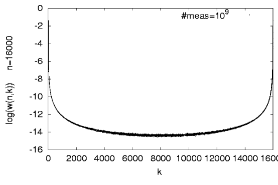
Figure 4: (a) $w(n,k)$ for $n=16000$ plotted from Eq. (31) and by application of our program routine ${\rm 10}^{\rm 9}$ times. (b) The deviation $\Delta w(n,k)=(w(n,k)_{\rm theoretical}-w(n,k)_{\rm measured})/w(n,k)_{\rm theoretical}$ using the same parameters.

and extra care must be put in the computer program so that we obtain the correct probabilities due to overflow. For this reason we have tested the distributions of $k$ for given $n$ obtained from the computer versus the theoretical value Eq. (31). The results for $n=16000$ are shown in fig. 4(a) where we plot $w(n,k)$ from Eq. (31) together with the results obtained from using our program ${\rm 10}^{\rm 9}$ times. A measure of the agreement is shown in fig. 4(b) where we plot the relative deviation $\Delta w(n,k)=(w(n,k)_{\rm theoretical}-w(n,k)_{\rm measured})/w(n,k)_{\rm theoretical}$. In the latter case, the data is smoothed using Savitzky-Golay filters to interpolate the nearest 100 points to a 4th order polynomial. As is seen, the distribution is symmetrical and the relative errors average out to 0 very nicely indicating that the deviation is pure statistical noise. We have checked that $|\Delta w(n,k)|\sim N_{\rm measurements}^{-0.5}$.

4 Numerical results

4.1 The fractal dimension

We have measured the fractal dimensions $d_{H}$ and $d_{h}$ in a number of ways to be described in the following. Since we are considering discretized, finite systems as approximations to continuum systems (although we try of course to stay as close to continuum physics as possible) it is important to use independent ways to approximate the same continuum physical observable. This will often give a more reliable idea of how close we are to the genuine continuum quantity since it supplements the systematic large $N$ study of a single choice of discretization of the continuum observable, where systematic cancellation of fluctuations might sometimes underestimate the real discrepancy between the measured quantity and the unknown value of the continuum observable.

4.1.1 Short distance behaviour

One can try to use directly the short distance behaviour (29) of $n_{N}(r)$ to extract $d_{h}$. This was the method used in the pioneering work [16]. The problematic aspect of the method is to what extend one has to take seriously the natural requirement $1\ll r\ll N^{1/d_{H}}$. We know now from the exact solution of pure two-dimensional quantum gravity that both limits have to be respected quite seriously, but that a so-called shift $r\to r+a$ helps to almost remove the requirement for the lower limit [11]. Later we will discuss various theoretical and “phenomenological” motivations for this shift. Presently, let us just use it as an additional fit parameter. In table 1 and table 2 we have shown the results of a fit of the form

$$n_{N}(r)=C\,(r+a)^{d_{h}-1},$$ (35)

for various cuts of $r_{\rm min}\leq r\leq r_{\rm max}$. We see here a discrepancy between $d_{h}$ obtained from the link-distance measurements and the triangle-distance measurements, respectively. If there is a discrepancy between the measured $d_{h}$ for triangle and link distance for finite $N$ one would expect it to be “maximal” when we concentrate on small $r$, like here. For small $r$ the triangle distance is quite rigid in the sense that each triangle has at most three neighbours, while a vertex can have any number of neighbouring vertices. This rigidity is also reflected in the fact that we have to use a much larger shift $a$ for triangle-distances. There is a weak tendency for the link–$d_{h}$ to decrease with $N$ while the triangle–$d_{h}$ shows a similar weak tendency to increase with $N$. From this one would conservatively estimate, assuming that they have a common large $N$ limit, that

$$3.53<d_{h}<3.60.$$ (36)

In figs. 5a and 5b we have shown the behaviour of short distance behaviour of $n_{N}(r)$ for the two distance measures and the whole range of $N$.

We will now show that the discrepancy between link–$d_{h}$ and triangle–$d_{h}$ indeed decreases when we use the finite size scaling (30) to invoke the whole range of $r$ and also that we can get a much better determination of $d_{h}$.

4.1.2 Collapse of distributions

Before using the finite size scaling relation (30) let us motivate the use of the “shift” $a$ which is essential for obtaining high precision results. The need of this parameter is well known from earlier studies of conformal field theories with $c\geq 0$ coupled to quantum gravity [11, 13]. One obvious, “phenomenological”, motivation for this shift parameter (which we have just copied from standard finite size scaling theory) is as follows: for finite $N$ we expect some discrepancy compared to continuum results, typically parameterised by “the number of points” $L$ corresponding to the linear size of the system. In particular we can write

$$x=\frac{R}{V^{1/d_{H}}}\sim\frac{r}{N^{1/d_{H}}}+\frac{{\rm const.}}{L}+\frac{{\rm const.}}{L^{2}}+\cdots,$$ (37)

or, since $N^{1/d_{H}}$ is precisely a typical measure for the linear extension of the system:

$$x=\frac{R}{V^{1/d_{H}}}\sim\frac{r+a}{N^{1/d_{H}}}+\frac{{\rm const.}}{(N^{1/d_{H}})^{2}}+\cdots.$$ (38)

The parameter $a$, which is considered a shift in r, incorporates the first order correction. Below we derive a theoretical value for $a$ in the case of pure gravity and where we use triangle distance. However, here we consider it as a purely phenomenological parameter, which in principle can be different for different scaling variables and will be different if we use different distance measures (viz. link and triangle distances).

The raw measurements of $n_{N}(r)$ produces distributions with $N$ ranging from $1K$ to $512K$. We can now try to fit them to the scaling ansatz (30). We have two parameters available, $d_{H}$ and $a$.

The collapse of the distributions is performed by using two different methods. The first one is identical to the one proposed in [10] and used with great success also in [13, 17]. One makes a non linear fit of the form $p_{n}(x){\rm e}^{-mx}$, where $p_{n}(x)$ is a polynomial of order $n$ in $x$, to the rescaled according to Eq. (30) distributions $n_{N}(r)$ for a given set of lattice sizes $\{N\}$. The $\chi^{2}(a,d_{H})$ per degree of freedom is computed for a given set of parameters $a$ and $d_{H}$. For each value of the shift $a$, the optimal value of $d_{H}$ is computed from the position of $\chi^{2}_{\rm min}(a)$.

We also used a second method which has the advantage of being much faster. We should also note that it is also quite successful even for very small lattices ($N<500$) where the fits used in the first method fail to yield reasonable results. For a given set of lattice sizes $\{N\}$ and parameters $(a,d_{H})$ we compute a cubic spline interpolation to the rescaled distribution for each value of $N$. $\chi^{2}(a,d_{H})$ is computed by adding in quadrature the distances of each point of the other distributions from the interpolation function reweighted by their errors and properly normalised to correspond to a $\chi^{2}$ per degree of freedom. The best values for $d_{H}$ computed this way are identical to the ones computed using the first method, although $\chi^{2}(a,d_{H})$ is slightly smaller and steeper yielding smaller errorbars ($\approx$ 10–30%) for the computed quantities. In this paper we report the larger errors computed from the first method.

In table 3 we have shown the results of the best fits both for the link-distance distribution and the triangle-distance distribution. The fits are divided into groups: the upper one determine $d_{H}$ and $a$ by comparing distributions $n_{N}(r)$ for successive pairs of $N$’s ($16K$ and $32K$, $32K$ and $64K$, etc.) In this way the $(d_{H},a)$ dependence on $N$ becomes clear. The middle and lower groups joins three, respectively four successive $N$’s in the determination of $d_{H}$ and $a$. In particular for the top group we see that $d_{H}$ has a clear dependence on $N$: If we use link distances $d_{H}(N)$ is systematically decreasing, while $d_{H}(N)$ is systematically increasing if we use triangle distances. Under the assumption that the trend will continue for larger systems and that the two distance measures are proportional to the genuine continuum distance in the scaling limit we conclude that

$$3.55<d_{H}<3.61.$$ (39)

These values of $d_{H}$ (and the appropriate values of $a$) actually yield excellent finite size scaling for the whole range of $N$ is illustrated in fig. 6a where we have shown $F^{(N)}_{1}(x)$ for the whole range of $N$ from $2K-256K$. The importance of the inclusion of the shift $a$ if we use the triangle distance is illustrated in fig. 6b where we have plotted the functions $F^{(N)}_{1}(x)$ obtained from $n_{N}(r)$ with the same choice of $d_{H}$ but with $a=0$. The same plots are shown in fig. 7a-7b in the case where we use the link distance. Here $a$ is smaller and not of the same visual importance as for triangle distances. However, in the actual fits they play an important role for the link distances as well if we want to extract consistent values of $d_{H}$ with acceptable $\chi^{2}$ values for the fits. In fig. 8 we see that the value of $d_{H}$ depends strongly on $a$.

However, we can use the systematic behaviour of $d_{H}$ as a function of $N$ and the shift parameter $a$ to obtain a better estimate of $d_{H}$ than the one provided by (39). In fig. 9 we have shown the complete $\chi^{2}_{\rm min}(a)$ fit which was used in the top group of table 3. Each point on the two subfigures represents a specific choice of the shift $a$. For a given $N$ we now find the value $d_{H}(a,N)$ which minimises the $\chi^{2}$ of the collapse of the $n_{N}(r)$ and $n_{N/2}(r)$. In table 3 we recorded just the minimum as a function of $a$ and the change of the minimum as a function of $N$ is seen quite clearly in fig. 9. However, let us for each $N$ plot the $d_{H}(a,N)$ of fig. 9 as a function of the shift $a$. This is shown in fig. 8. We get a number of straight lines which with very good accuracy intersect for one value of $a_{0}$. The simplest phenomenological explanation of this fact is that $a_{0}$ is the correct value from (39), since this implies that

$$d_{H}(a,N)=d_{H}(a_{0},\infty)+\left[\frac{\partial d_{H}(a_{0},\infty)}{\partial a}+\frac{\partial^{2}d_{H}(a_{0},\infty)}{\partial a_{0}\partial(1/N)}\,\frac{1}{N}\right](a-a_{0})+\cdots.$$ (40)

From this argument the correct infinite volume limit of $d_{H}$ is determined from the figures up to the accuracy with which the curves actually cross in a single point. This interpretation confirmed by the fact that both the triangle and link $d_{H}(a,N)$ curves cross at the same value of $d_{H}$, but for very different $a_{0}$.

We conclude from the data (see figure) that

$$d_{H}=3.57\pm 0.01\,.$$ (41)

4.1.3 Average radius

In this section we will use the average radius of a universe to extract the intrinsic Hausdorff or fractal dimension. From the definition of $n_{N}(r)$ the average radius of universes with volume $N$ is

$$\left\langle r\right\rangle_{N}\equiv\frac{1}{N}\sum_{r=0}^{\infty}r\;n_{N}(r)\sim N^{1/d_{H}}\,.$$ (42)

Obviously, (42) could itself serve as a natural definition of $d_{H}$. By measuring $n_{N}(r)$ we can record $\left\langle r\right\rangle_{N}$ as a function of $N$ and hence determine $d_{H}$. As usual we have to introduce the shift $a$ in order to account for lowest order discretization effects. Now, let us define

$$R_{a,N}(d)=\frac{\left\langle r+a\right\rangle_{N}}{N^{1/d_{H}}}\,.$$ (43)

We determine the values of $a$ and $d_{H}$ in the following way: first we measure $\left\langle r\right\rangle_{N_{i}}$ for a certain number of different volumes $N_{i}$ of the universes, ranging from $N=2K$ to $N=256K$. For a given $a$ we choose, for each couple $N_{i},N_{j}$ of $N$’s, the $d_{H}^{ij}$ such that

$$R_{a,N_{i}}(d_{H}^{ij})=R_{a,N_{j}}(d_{H}^{ij})\,.$$ (44)

For this choice of $N_{i},N_{j}$ we bin the data and estimate an error $\delta d_{H}^{ij}$. Then we determine the average

$$\bar{d}_{H}=\frac{1}{{\rm\#~{}pairs}}\sum_{i\neq j}d_{H}^{ij}\,,$$ (45)

and compute

$$\chi^{2}(a)=\frac{1}{{\rm\#~{}pairs}}\sum_{i\neq j}\frac{(d_{H}^{ij}-\bar{d}_{H})^{2}}{(\delta d_{H}^{ij})^{2}}\,.$$ (46)

The preferred pair $(a,d_{H}(a))$ is determined by the minimum of $\chi^{2}(a)$. This method works quite impressively. In fig. 10a and fig. 10b we have shown the intersection of the curves $R_{a,N}(d)$ as a function of $d$ for the optimal choice of $a$ for link–distance and triangle–distance measurements, respectively. The important points are that in both cases there exists a value of $a$ where all the curves intersect with high precision, and that the range of $a$ where $\chi^{2}(a)$ is acceptably small, i.e. $O(1)$, is quite small. Hence $d_{H}$ is determined with high precision. In Fig. 11a and 11b we show $\chi^{2}(a)$ for link–distance and triangle distance measurements, respectively. In this way we get

$$d_{H}(a_{m})=3.573\pm 0.005\,$$ (47)

both from the link–distance measurements and the triangle–distance measurements. The values of $a_{m}$ are

$$a_{m}=0.13\pm 0.01\,,~{}~{}~{}~{}~{}{\rm and}~{}~{}~{}~{}~{}a_{m}=5.00\pm 0.05,$$ (48)

for the link–distance and triangle–distance, respectively. In table 4 we have listed the determination of $(d_{H}(a_{m}),a_{m})$ for various cuts in the lower values of $N$. The constancy and consistency of the results are truly remarkable.

In (47) we have estimated the error as follows. Define an interval of acceptance $[a_{\rm min},a_{\rm max}]$ of $a$ by demanding that $\chi^{2}(a)<2\chi^{*}$ where $\chi^{*}={\rm max}\{1,\chi^{2}(a_{m})\}$ and find the variation of $d(a)$ in this interval. After this we repeat the whole procedure by making various cuts in the pairs of $N_{i}$’s included in (45) and (46), discarding successively the smallest $N_{i}$’s.

We note that the values (47) are in perfect agreement with (41). We have now four independent measurements (two different methods, two different definitions of length) which all give $d_{H}=3.57\pm 0.01$.

4.2 Boundaries

We now turn to the measurements of $\left\langle l^{n}\right\rangle_{r,N}$. These observables are constructed from $\rho_{N}(l,r)$, which can readily be measured in the simulations. We recall the situation in pure two-dimensional quantum gravity which can be solved explicitly and where $d_{h}=4$. In this case we have (for small $r$):

$$\left\langle l\right\rangle_{r,N}^{c=0}\sim r^{3},~{}~{}~{}~{}\left\langle l^{n}\right\rangle_{r,N}^{c=0}\sim r^{2n},~{}~{}n>1.$$ (49)

Since $d_{h}=4$ in this case, i.e. $\left\langle r^{2n}\right\rangle\sim N^{n/2}$, we obtain

$$\left\langle l^{n}\right\rangle_{r,N}^{c=0}\sim\Bigl{(}\sqrt{N}\Bigr{)}^{n},~{}~{}~{}n>1,$$ (50)

as one naively would have expected for a smooth two-dimensional world. Only the first moment behaves anomalous, as it has to do if $d_{h}\neq 2$. From these $c=0$ considerations it is unclear what to expect for $c=-2$ for the higher moments. If ${\rm dim}[\,N\,]={\rm dim}[\,l^{2}\,]$, then from scaling arguments, we expect

$$\left\langle l^{n}\right\rangle_{r,N}\sim N^{n/2}\tilde{F}_{n}(x)\,,~{}~{}~{}~{}~{}x=\frac{r}{N^{1/d_{H}}}\,.$$ (51)

However, our measurements are consistent with the following scaling relations

$$\left\langle l^{n}\right\rangle_{r,N}\sim N^{2n/d_{H}}F_{n}(x),~{}~{}~{}~{}~{}{\rm for}~{}~{}n\geq 2\,,$$ (52)

which implies that ${\rm dim}[\,l^{n}\,]={\rm dim}[\,r^{2n}\,]$ for $n>1$. Eq. (52) indicates that we have

$$\left\langle l^{n}\right\rangle_{r,N}\sim r^{2n}~{}~{}~{}~{}~{}{\rm for}~{}~{}1\ll r\ll N^{1/d_{H}},~{}n\geq 2\,.$$ (53)

We have shown this relation in fig. 12 for $n=2$, $3$ and $4$ for the case where we use link distances. It is remarkably well satisfied. In table 5 we have shown the more detailed result of this short distance analysis. It should be compared to the short distance analysis presented in table 2 (and fig. 5b) for the first moment. The behaviour of the exponents $2n$ for the higher moments as functions of $N$ are clearly more consistent and systematic compared with the behaviour of $d_{H}(N)$ for the first moment. In addition one can use smaller values of $r$ and there is not the same crucial dependence on the shift $a$ as for the first moment. All this points consistently to smaller short-distance discretization effects for the higher moments. Note also that the value of the shift $a$ is different.

Let us now turn to the finite size scaling analysis of (52). Again we introduce as a first phenomenological correction the shift $r\to r+a$ as in (43) to find the best scaling function $F_{n}(x)$ for a suitable range of $N_{i}$’s. We have shown $F_{n}(x)$ for $n=2,3$ and 4 for the values of $a$ which provide the best scaling function in fig. 13. The more detailed analysis is given in table 6. Note that the results are perfectly consistent with the same analysis for the first moment (table 2), but the shift $a$ is different and in fact not very well determined (see fig. 14). In principle this is a good thing, but it implies that we cannot use the shift in the same constructive way as for the first moment and get a high precision measurement of $d_{H}$.

The scaling ansatz (51) seems to be ruled out. In fig. 15a we have shown the best overlap functions $\tilde{F}_{2}(x)$ for the second moment $\left\langle l^{2}\right\rangle_{r,N}$ using (51). It should be compared to fig. 13, where we have used the ansatz (52). Clearly (52) is superior to (51). One may, however, consider the possibility of a dimensional relation of the form:

$${\rm dim}[\,l^{n}\,]={\rm dim}[\,r^{2n(1-\epsilon)}\,]\,.$$ (54)

In this case, for given $d_{H}$, one can use the relation $\left\langle l^{n}\right\rangle_{r,N}=N^{2n(1-\epsilon)/d_{H}}F_{n}(x)$ in order to determine the value of $\epsilon$. We get an upper bound on $\varepsilon$ by using the lowest value of for $d_{H}$ (obtained by some of the other methods discussed above) and then fitting to the data. In this way we obtain $\epsilon<0.03$. We consider the existence of such a small $\epsilon\neq 0$ unnatural.

4.3 Distribution function

Let us finally turn to the measurement of the distribution function $\rho_{N}(r,l)$, which provides the complete information about the moments $\left\langle l^{n}\right\rangle_{r,N}$. In the case of pure gravity one can calculate $\rho_{N}(r,l)$ in the limit $N\to\infty$ and one finds [6]:

$$\rho^{(c=0)}_{\infty}(r,l)\sim\frac{1}{r^{2}}G^{(c=0)}(l/r^{2}),$$ (55)

where the function $G^{(0)}(z)$ is

$$G^{(0)}(z)=\Bigl{(}\frac{1}{z^{5/2}}+\frac{1}{2z^{3/2}}+\frac{14z^{1/2}}{3}\Bigr{)}\;{\mathrm{e}}^{-z}.$$ (56)

Note that this form of $\rho^{(0)}_{\infty}(r,l)$ explains (49). If $\varepsilon$ denotes the cut-off (the lattice spacing in the triangulation) we can write

$$\left\langle l^{n}\right\rangle_{r,N=\infty}^{c=0}=\int_{\varepsilon}{\mathrm{d}}l\,l^{n}\rho^{(0)}_{\infty}(r,l)=r^{2n}\int_{\varepsilon/r^{2}}{\mathrm{d}}z\,z^{n}G^{(0)}(z).$$ (57)

For $n>1$ the lower limit has no implication for the integral and can be dropped. However, for $n=1$ the leading contribution in the limit $\varepsilon\to 0$ comes precisely from the lower integration limit and we obtain:

$$\left\langle l\right\rangle_{r,N=\infty}^{c=0}\sim\frac{1}{\varepsilon^{1/2}}\;r^{3}.$$ (58)

The cut–off dependence ensures that the real dimension of $\left\langle l\right\rangle$ is equal to that of $\sqrt{N}$.

Since we have verified with good accuracy that the higher moments for $c=-2$ and $c=0$ has the same $r$ dependence for large $N$ (see (49) and (53)), we know that

$$\rho_{N}(r,l)\sim\frac{1}{r^{2}}G(l/r^{2})~{}~{}~{}~{}~{}\hbox{for ~{} $N\to\infty$}.$$ (59)

The function $G(z)$ need not be identical to $G^{(0)}(z)$. In fact it cannot be identical since $d_{h}(c=-2)\neq d_{h}(c=0)$. Since we expect that the origin of the different behaviour of the first and the higher moments is the same for $c=0$ and $c=-2$ we know that the small $z$ behaviour of $G(z)$ must be

$$G(z)\sim\frac{1}{z^{(d_{h}+1)/2}},~{}~{}~{}~{}d_{h}\approx 3.57.$$ (60)

Fig. 16a displays that the link-distance distribution function $r^{2}\rho_{N}(r,l)$ is to a good approximation only a function of $z=l/r^{2}$ as long as $r/N^{1/d_{H}}<1$. For small values of $z$ the $\log(G(z))$–curve is approximately a linear function of $\log(z)$. From (60) we expect

$$\log G(z)\sim-\,\frac{d_{h}+1}{2}\log z~{}~{}~{}~{}~{}\hbox{for ~{} $\log z\to-\infty$}.$$ (61)

A measurement of the slope gives $d_{h}=3.60\pm 0.03$ in good agreement with short distance behaviour $\left\langle l\right\rangle_{r,N}$, as given in table 2 for the link distance. We emphasise that this agreement is no surprise. There has to be agreement. However, as we have seen, some treatments of the data set can produce very precise measurements of $d_{h}$. The slope of $\log G(z)$ does not belong to this class.

Finally, in fig. 16c, we have shown $r^{2}\rho_{N}(r,l)$ in a somewhat larger $z$ interval. We know from measurements of the large $r$ behaviour of the moments $\left\langle l\right\rangle_{r,N}$ that they fall off fast when $x=r/N^{1/d_{H}}>1$ (see (51) and fig. 13a-13c). The same behaviour has to be coded in $\rho_{N}(r,l)$. The simplest guess:

$$\rho_{N}(r,l)\sim\frac{1}{r^{2}}G(z)H(x)$$ (62)

is not satisfied since this would imply that the scaling functions $F_{n}(x)$ were proportional to $x^{2n}H(x)$, which is not very well satisfied numerically. However, the ansatz (62) is not too far from the truth either. Since the curves shown in fig. 16c are very similar to the ones for pure gravity one can test that an ansatz like (62), replacing $G(z)$ with $G^{(0)}(z)$ and $H(x)$ with the function $f(x)$ from (23). The ansatz will produce curves qualitatively very similar to the ones shown in fig. 16c. Indeed, the curves consists of three major parts. Let $y=\log l/r^{2}$. The right part of the curve goes as $-e^{y}$ and comes from the exponential decay of $G^{(0)}(l/r^{2})$ for positive $y$. The “straight-line part” is $-(5/2)y$ which dominates for negative $y$, as discussed above. The “bump” is the joining of these two asymptotic regions. Finally, for fixed $l/N^{2/d_{H}}$ and large negative $y$ we hit the region where $f(x)$ goes to zero. It will contribute with a term (for $d_{H}=4$)

$$-\Bigl{(}\frac{l}{N^{1/2}}\Bigr{)}^{2/3}{\mathrm{e}}^{-\frac{2}{3}y}.$$ (63)

This term depends on $l/N^{2/d_{H}}$ and consequently the decay of $\rho_{N}(r,l)$ for large negative $y$ will depend on $l/N^{2/d_{H}}$ precisely as is shown for the $c=-2$ case in fig. 16c.

5 Theoretical estimate on the finite size shift of geodesic distance

In eq. (38) we introduced the shift as part of a general finite size expansion. Since it plays an important role in the fits it is worthwhile to provide a theoretical understanding of the magnitude of the shift. We shall limit ourselves to an analysis of the $c=0$ model where it is possible to perform a theoretical analysis at a discretized level. There are other technical differences between the theoretical and the numerical analyses which will be explained in order. Thus the comparison will be qualitative. Yet we believe that the present analysis provides a theoretical confirmation of the existence of a finite size shift of the geodesic distance.

The finite size shift $a$ will be shown to incorporate the effect of next higher-order correction in a lattice spacing parameter. Here, we denote the two-point functions at the discrete level and at the continuous level as $G_{g}(r)$ and $G_{\mu}(R)$, respectively. The two-point functions are related with $S_{V}(R)$ and $n_{N}(r)$ as

$$G_{\mu}(R)=\int\!dVe^{-\mu V}VZ(V)S_{V}(R),~{}~{}~{}~{}~{}G_{g}(r)=\sum_{N}g^{N}NZ_{N}\,n_{N}(r),$$ (64)

where we have introduced $g$ as a coupling constant of matrix model, $r$ as the geodesic distance in the discrete level, $\mu$ as the cosmological constant, and $R$ as the geodesic distance at the continuous level. $g$ and $r$ are related with $\mu$ and $R$ by $g=g_{c}e^{-\alpha\varepsilon^{2}\mu}$ and $R=\beta r\varepsilon^{2\nu}$, where $\alpha$ and $\beta$ are constant, and $\varepsilon$ is the lattice spacing parameter in the triangulation.

According to the arguments in ref. [7], the continuum limit of the two-point function is

$$G_{g}(r)=\varepsilon^{2(\eta-1)\nu}\Bigl{\{}G_{\mu}(R)+\varepsilon^{2\nu}G_{\mu}^{(1)}(R)+O(\varepsilon^{4\nu})\Bigr{\}}\,,$$ (65)

where $\nu$ and $\eta$ are constant. Suppose that the following relation

$$G_{\mu}^{(1)}(R)=\beta a\frac{\partial}{\partial R}G_{\mu}(R)\,,$$ (66)

is satisfied, we obtain

$$G_{g}(r)=\varepsilon^{2(\eta-1)\nu}\Bigl{\{}G_{\mu}(R+\beta a\varepsilon^{2\nu})+O(\varepsilon^{4\nu})\Bigr{\}}\,,$$ (67)

where this $a$ will be identified as the finite size shift of geodesic distance. Thus, one can incorporate next higher-order correction by redefining the geodesic distance at the continuous level by $R^{\rm modified}=\beta(r+a)\varepsilon^{2\nu}$ instead of by simply taking $R=\beta r\varepsilon^{2\nu}$.

Now, let us carry out a concrete calculation. Here, we restrict to the analysis of pure gravity ($c=0$ model) because this is the only case where the two-point function is theoretically known as a function of the geodesic distance $R$. In defining geodesic distance at the discrete level, there are two types of decomposition of triangles; slicing decomposition [6] and peeling decomposition [23]. $G_{\mu}(R)$ is known for both cases while the discrete two-point function $G_{g}(r)$ is known only for the case of the peeling decomposition. In the peeling process, a triangle can be peeled off with $1/l$ step forward of geodesic distance ($l$: loop length at the discrete level) while full one step forward of geodesic distance is realized in the one slicing process.

In the peeling decomposition[23], the two-point function is related with the generating function of the disk amplitude at the discrete level [7],

$$G_{g}(r)=\frac{\partial}{\partial x}F_{g}(\hat{x}(x,r))\bigg{|}_{x=0}=\frac{1}{g}\frac{\partial}{\partial r}F_{g}(\hat{x}(0,r))\,,$$ (68)

where we start from the boundary of disk with length $l_{1}=1$ at $r=0$. Here, $F_{g}(x)=\sum_{l}x^{l}F_{g}(l)$ is the generating function of the disk amplitude $F_{g}(l)$ with one marked link and boundary length $l$ at the discrete level. The function $\hat{x}(x,r)$ satisfies $\hat{x}(x,r=0)=x$ and

$$\frac{\partial\hat{x}}{\partial x}=\frac{f_{g}(\hat{x})}{f_{g}(x)}\,,~{}~{}~{}~{}~{}\frac{\partial\hat{x}}{\partial r}=gf_{g}(\hat{x})\,.$$ (69)

In the case of one-matrix model[24], $F_{g}(x)$ and $f_{g}(x)$ have the following forms,

$$F_{g}(x)=\frac{1}{2}\biggl{(}\frac{1}{x^{2}}-\frac{g}{x^{3}}\biggr{)}+\frac{g}{2x^{3}}f_{g}(x)\,,~{}~{}~{}f_{g}(x)=(1-c_{2}x)\sqrt{(1-c_{1}x)(1-c_{0}x)}\,,$$ (70)

where $c_{0}<0<c_{1}<c_{2}$. The solution of (69) is[7]

$$\hat{x}(x,r)=\frac{1}{c_{2}}\Biggl{\{}1-\frac{\delta_{1}}{\sinh^{2}\bigl{(}\delta_{0}r+\sinh^{-1}\!\sqrt{\frac{\delta_{1}}{1-c_{2}x}-\delta_{2}}\bigr{)}+\delta_{2}}\Biggr{\}}\,,$$ (71)

where

$$\delta_{0}=\frac{g}{2}\sqrt{(c_{2}-c_{1})(c_{2}-c_{0})},~{}~{}~{}\delta_{1}=\frac{(c_{2}-c_{1})(c_{2}-c_{0})}{c_{2}(c_{1}-c_{0})},~{}~{}~{}\delta_{2}=-\,\frac{c_{0}(c_{2}-c_{1})}{c_{2}(c_{1}-c_{0})}.$$ (72)

Next, let us consider to take the continuum limit of (68). The continuum limit of the disk amplitude is taken by imposing $x=x_{c}e^{-\varepsilon\zeta}$ and $g=g_{c}e^{-\alpha\varepsilon^{2}\mu}$,

$$F_{g}(x)={\rm(const.)}\varepsilon^{3/2}\Bigl{\{}-b_{1}\varepsilon^{-3/2}-b_{2}\varepsilon^{-1/2}\zeta+f_{\mu}(\zeta)+O(\varepsilon^{1/2})\Bigr{\}}\,,$$ (73)

$$~{}~{}~{}~{}~{}~{}f_{\mu}(\zeta)=\Bigl{(}\zeta-\frac{\sqrt{\mu}}{2}\Bigr{)}\sqrt{\zeta+\sqrt{\mu}}\,,$$ (74)

where the constants, $b_{1}$ and $b_{2}$, and the critical values, $x_{c}$ and $g_{c}$, are regularization dependent. The continuum limit of $\hat{x}(0,r)$ is

$$\hat{x}(0,r)=x_{c}\Bigl{\{}1-\varepsilon\hat{\zeta}_{0}(R+\beta a_{1}\sqrt{\varepsilon})+O(\varepsilon^{2})\Bigr{\}}\,,$$ (75)

where

$$\hat{\zeta}_{0}(R)=-\sqrt{\mu}+\frac{3}{2}\sqrt{\mu}\coth^{2}\biggl{(}\sqrt{\frac{3}{2}}\mu^{1/4}R\biggr{)}\,,$$ (76)

and $R=\beta r\sqrt{\varepsilon}$, which means that $\nu=1/4$ in pure gravity. Substituting (73) and (75) into (68), we find

$$G_{g}(r)={\rm(const.)}\varepsilon^{3/2}\frac{\partial}{\partial R}\biggl{\{}-b_{2}\hat{\zeta}_{0}(R+\beta a_{1}\sqrt{\varepsilon})+\sqrt{\varepsilon}f_{\mu}\bigl{(}\hat{\zeta}_{0}(R)\bigr{)}+O(\varepsilon)\biggr{\}}\,,$$ (77)

which tells us that $\eta=4$. Here, we obtain the following nontrivial relation from (76),

$$\frac{\partial}{\partial R}\hat{\zeta}_{0}(R)=-2f_{\mu}(\hat{\zeta}_{0}(R))\,.$$ (78)

Then we find the property (66), i.e., we finally find

$$G_{g}(r)=-{\rm(const.)}\varepsilon^{3/2}\frac{\partial}{\partial R}\biggl{\{}\hat{\zeta}_{0}\Bigl{(}R+\beta a_{1}\sqrt{\varepsilon}+\frac{\sqrt{\varepsilon}}{2b_{2}}\Bigr{)}+O(\varepsilon)\biggr{\}}\,.$$ (79)

Thus, we obtain

$$R^{\rm modified}=\beta(r+a)\varepsilon^{2\nu}~{}~{}~{}\hbox{where}~{}~{}~{}a=a_{1}+a_{2},\biggl{(}a_{2}=\frac{1}{2b_{2}\beta}\biggr{)}\,.$$ (80)

In the one-matrix model which describes pure gravity, the critical values are $x_{c}=(3^{1/4}-3^{-1/4})/2$ and $g_{c}=1/(2\cdot 3^{3/4})$. Then, we find $b_{2}=\sqrt{3}(\sqrt{3}+1)^{-3/2}$, $\beta=(\sqrt{3}+1)^{1/2}/(2\sqrt{3})$, and $a_{1}=\sqrt{3}$. Therefore, the total finite size shift becomes

$$a=a_{1}+a_{2}=2\sqrt{3}+1=4.46...~{}~{}~{}(a_{1}=\sqrt{3},~{}a_{2}=\sqrt{3}+1)\,.$$ (81)

We now try to evaluate the two-point function where the starting boundary length is $3$ at $r=0$. In this case we have to take the third derivative of the generating function of the disk amplitude instead of the first derivative of (68),

$$G^{[l_{1}=3]}_{g}(r) = \frac{1}{3!}\biggl{(}\frac{\partial}{\partial x}\biggr{)}^{3}F_{g}(\hat{x})\bigg{|}_{x=0}$$

$$= \frac{1}{3!}\Biggl{\{}\biggl{(}\frac{1}{f_{g}}\biggr{)}^{\prime\prime}+\frac{3}{g}\biggl{(}\frac{1}{f_{g}}\biggr{)}^{\prime}\frac{\partial}{\partial r}+\frac{1}{g^{2}}\biggl{(}\frac{\partial}{\partial r}\biggr{)}^{2}\Biggr{\}}\frac{1}{g}\frac{\partial}{\partial r}F_{g}(\hat{x})\bigg{|}_{x=0}\,.$$

The continuum limit of (5) is

$$G_{g}^{[l_{1}=3]}(r)={\rm(const.)}\biggl{(}1+\beta a_{3}\sqrt{\varepsilon}\frac{\partial}{\partial R}+O(\varepsilon)\biggr{)}G_{g}^{[l_{1}=1]}(r)\,,$$ (83)

where $G_{g}^{[l_{1}=1]}(r)$ is $G_{g}(r)$ of (79) and

$$a_{3}\ =\ \lim_{\varepsilon\rightarrow 0}\frac{3(1/f_{g})^{\prime}}{g(1/f_{g})^{\prime\prime}}\bigg{|}_{x=0}\,.$$ (84)

In the one-matrix model, the value of $a_{3}$ is $a_{3}=3/2$. For the case with the boundary disk length $l_{1}=3$ at $r=0$, we obtain the total finite size shift,

$$a=a_{1}+a_{2}+a_{3}=2\sqrt{3}+\frac{5}{2}=5.96...\,.$$ (85)

The similar calculation can be done for the triangulation without two-folded links (two links are on top of each other) which come from the kinetic term in the matrix model. In this case the disk amplitude is

$$F_{g}(x)=\frac{x}{2g}-\frac{1}{2}-x^{2}+\frac{1}{2}f_{g}(x)\,,~{}~{}~{}f_{g}(x)=(1-c_{2}x)\sqrt{1-c_{1}x}\,,$$ (86)

where $c_{1}=4/(gc_{2}^{2})$ and $c_{2}^{3}-c_{2}/g^{2}=-8/g$. Since $f_{g}(x)$ in (86) is formally the same as $f_{g}(x)$ in (70) with the substitution $c_{0}=0$, $\hat{x}(x,r)$ of the present model is formally the same as $\hat{x}(x,r)$ in (71) with $c_{0}=0$. In this case, the continuum limit is realized around the critical values, $x_{c}=1/(2\cdot 3^{1/4})$ and $g_{c}=1/(2\cdot 3^{3/4})$. The continuum limit of $F_{g}(x)$ is (73) with $b_{2}=2/\sqrt{3}$, and that of $\hat{x}(0,r)$ is (75) with $\beta=1/(2\sqrt{3})$ and $a_{1}=2\sqrt{3}$. Then, for the present model we find

$$a=a_{1}+a_{2}=2\sqrt{3}+\frac{3}{2}=4.96...~{}~{}~{}(a_{1}=2\sqrt{3},~{}a_{2}=\frac{3}{2})\,.$$ (87)

In the present case with the boundary disk length $l_{1}=3$ at $r=0$, the total finite size shift is

$$a=a_{1}+a_{2}+a_{3}=\frac{16\sqrt{3}}{5}+\frac{3}{2}=7.04...\,,$$ (88)

where $a_{3}=6\sqrt{3}/5$ which is derived from (84).

In the slicing decomposition in pure gravity[6], we have $a_{2}=\sqrt{(38+21\sqrt{3})/6}$, because of the property that (78) is independent of regularization. However, we failed to obtain $a_{1}$ because we do not know the concrete expression of $\hat{x}(x,r)$ in the slicing decomposition.

The above arguments show that the finite size shift $a$ depends on the detailed prescription for the starting point and the class of triangulations used. As a further source of ambiguity we can mention that the counting of distance in the theoretical considerations above and in numerical simulations differ in the following way: In our numerical simulations we first mark one of the triangles on the sphere, and then measure the distance from the marked triangle. The marked triangle might be a normal triangle or a triangle which corresponds to a tadpole in the dual lattice. Thus the marked point is located at the center of the marked triangle in our simulation while the boundary of the marked triangle is the zero geodesic region in the above theoretical analysis. In fig. 3 we describe the definitions of the distance both in the above theoretical analysis and in our numerical analyses. Therefore, the geodesic distance in the numerical simulation $r^{\rm sim}$ is related with the geodesic distance $r$ as $r^{\rm sim}\sim r+1/2$. Since $R^{\rm modified}=\beta(r+a)\varepsilon^{2\nu}=\beta(r^{\rm sim}+a^{\rm sim})\varepsilon^{2\nu}$, which reproduces the universal function $G_{\mu}(R^{\rm modified})$, we find $a^{\rm sim}\sim a-1/2$.

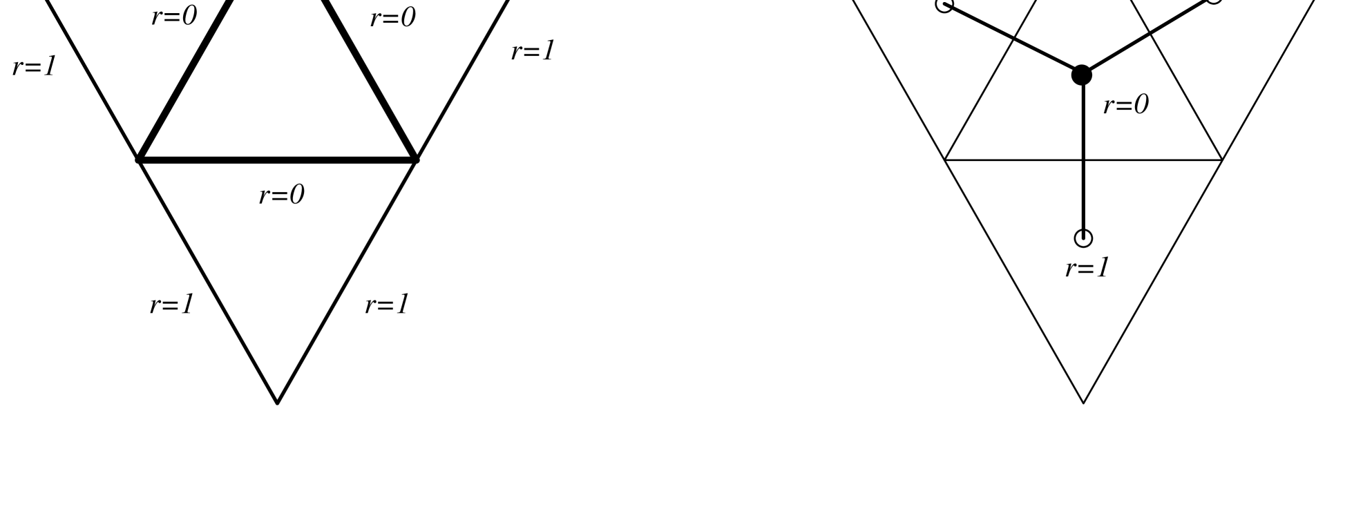
Figure 3: (a) The distance used in the theoretical analysis. (b) The distance used in our numerical simulation. The difference of the distances between (a) and (b) is about $1/2$.

Another slight difference between the theoretical and numerical determination of the shift $a$ is the different definition used for the boundary lengths. In the numerical simulations we count the number of triangles at a given distance $r^{\rm sim}$ whereas in the theoretical approach we count the number of links at distance $r$. Finally, in the computer simulations we use a modified version of the slicing decomposition. This implies that we cannot directly compare with the theoretical results derived above which use the peeling decomposition to estimate the geodesic distance $r$. However, when we compare with the numerical simulations with $c=0$ it is found that the shift is $4<a<6$ [11] which is consistent with eqs. (81),(85),(87) and (88).

For more general models where $c\neq 0$, we have not succeeded in showing the property (66) which is used in proving the existence of the shift $a$. On the other hand, the numerical simulation in $c\neq 0$ models strongly supports the existence of the shift $a$ of the same order of magnitude as for the $c=0$ model.

Finally, we consider the shift in $\langle l^{n}\rangle_{r}$. In the peeling decomposition, $\langle l^{n}\rangle_{r}$ is described by

$$\langle l^{n}\rangle_{r}=\frac{\partial}{\partial x}\biggl{(}\hat{x}\frac{\partial}{\partial\hat{x}}\biggr{)}^{n-1}F_{g}(\hat{x}(x,r))\bigg{|}_{x=0}\,,$$ (89)

where we start from the boundary of disk with length $l_{1}=1$ at $r=0$. Note that from (75) we obtain

$$\hat{x}\frac{\partial}{\partial\hat{x}}\ =\ -\,\frac{1}{\varepsilon}\frac{\partial}{\partial\hat{\zeta}_{0}}+O(\varepsilon)\,.$$ (90)

Substituting (90) into (89) and carrying out the similar calculation as before, we find for $n\geq 2$,

$$\langle l^{n}\rangle_{r}={\rm(const.)}\varepsilon^{3-n}\frac{\partial}{\partial R}\biggl{(}\frac{\partial}{\partial\hat{\zeta}_{0}}\biggr{)}^{n-1}\biggl{\{}f_{\mu}\bigl{(}\hat{\zeta}_{0}(R+\beta a_{1}\sqrt{\varepsilon})\bigr{)}+({\rm const.})\sqrt{\varepsilon}\Bigl{(}\hat{\zeta}_{0}(R)\Bigr{)}^{2}+O(\varepsilon)\biggr{\}}\,.$$ (91)

For $n\geq 3$ the finite size shift comes only from $a_{1}$ because $a_{2}$ is absent. When we start from the boundary of disk with length $l_{1}=3$ at $r=0$, the shift is $a_{1}+a_{3}$. The values of $a$ for $\langle l^{n}\rangle_{r}$ ($n\geq 3$) are all equal but are smaller than that of $a$ for $\langle l\rangle_{r}$ by $a_{2}$. On the other hand, for $n=2$ the property (66) is broken, because $\hat{\zeta}_{0}^{2}$ is not proportional to $(\partial/\partial R)f_{\mu}(\hat{\zeta}_{0})$. So, we cannot expect a clear shifting property for $\langle l^{2}\rangle_{r}$ in the numerical simulations.

6 Discussion

In this article we have taken advantage of the special recursive sampling possible for the $d=-2$ theory coupled to quantum gravity. The quality of the numerical data obtained this way is much better than the quality of data obtained with a similar computer effort by ordinary Monte Carlo simulations. The purpose of the present work has been to measure the fractal structure of space-time in the $c=-2$ theory coupled to quantum gravity with a precision which has not been available before, by combining the high quality data with the technique of finite size scaling.

In this way we obtained, with a conservative error estimate,

$$d_{H}=3.58\pm 0.04,~{}~{}~{}~{}~{}d_{h}=3.56\pm 0.04,$$ (92)

in perfect agreement with the theoretical prediction $3.561\cdots$ from the diffusion in Liouville theory (see (4) and (8)), and in disagreement with the prediction given by (1)-(3).

Thus eq. (4) is strongly favoured as the correct formula for the fractal dimension of space-time in the case where the matter fields coupled to gravity have $c<0$. In this region eq. (4) has nicer properties than eq. (1), since one naively expects that $d_{H}(c)\to 2$ for $c\to-\infty$. It is reassuring that (4), rather than (1), is selected as the correct formula, since $d_{H}$ in (4) goes to 2 for $d\to-\infty$. In addition (92) provides strong evidence for the existence of a unique fractal dimension $d_{H}=d_{h}$ at all distances. As shown in the Appendix one cannot take for granted such a relation, in particular for non–unitary theories coupled to quantum gravity, but based on (92) it is tempting to conjecture that, contrary to the situation for the so-called multi-critical branched polymers discussed in the Appendix, we will always have $d_{H}=d_{h}$ in quantum gravity.

We have emphasised the validity of (4) for $c\leq 0$, but have remained silent about the region $0<c<1$. The reason is that for non–unitary conformal field theories we have operators with negative scaling dimensions. They will be dominant relative to the cosmological term, and it cannot be entirely ruled out that a formula like (1) is correct for $c>0$. Contrary to eq. (4) it has a drastic dependence on $c$ for $c\to 1$. This dependence has not been observed until now in the computer simulations which favour $d_{H}\approx 4$. For $c>0$ the numerical data are based on ordinary Monte Carlo simulations and it is not possible to perform the same high precision determination of $d_{H}$ as for $c=-2$. The best present data are not in good agreement with (4), but cannot falsify it either.

Eqs. (52) and (53) show a new and surprising scaling indicating that $l/r^{2}$ seems to be a universal, dimensionless variable. In the case $c=0$ this is certainly reasonable since we know that the dimension of $r$ is $N^{1/4}$ and it is natural to expect that a boundary has dimension $N^{1/2}$. This is not satisfied for $\langle l\rangle_{r}$ due to the fractal structure of space-time, which implies that the boundary of a sphere of geodesic radius $r$ is highly multi-connected with many microscopic loops. This manifests itself in the short distance cut-off needed in eq. (57) for $n=1$. However, for moments $\langle l^{n}\rangle_{r}$, $n>1$, these microscopic loops play no role and we get $\langle l^{n}\rangle_{r}\sim N^{n/2}$ (see eq. (50)). If $l/r^{2}$ is a universal, dimensionless variable also for $c<0$ where $d_{H}<4$, we reach the conclusion that the $l$ appearing in the computer measurements cannot be identified with the “Liouville” $\ell$, which in the continuum notation is believed to have the dressing dictated by:

$$\delta(\int\!d^{2}\xi\sqrt{\hat{g}}\;e^{\alpha\phi}-V)\to\delta(\int\!d\xi\sqrt[4]{\hat{g}}\;e^{\alpha\phi/2}-\ell),$$ (93)

where $\alpha$ denotes the gravitational dressing associated with the cosmological term and the gravitational dressing of the boundary cosmological term is $\alpha/2$. In the context of Liouville theory it has never been entirely clear how to derive this result from first principles since the actual boundary conditions of the matter fields for $c<0$ have never been explicitly specified. In the numerical simulations the boundary is not fixed, but only characterised by being a (multi-connected) spherical shell of geodesic radius $r$. Probably free boundary conditions in Liouville theory come closest to the “experimental” set-up in the numerical simulations, and maybe the existence of scaling operators with negative dimensions in the non-unitary theories can spoil the relationship between the dimension of space-time and boundary shown in eq. (93) in the case of free boundary conditions, since these operators are dominant relative to the cosmological constant.

We hope it will eventually be possible to understand this new, observed scaling of the boundary length from first principles.

Acknowledgements

J. Ambjørn acknowledges the support of the Professor Visitante Iberdrola Grant and the hospitality at the University of Barcelona, where part of this work was done. Y. Watabiki acknowledges the support and the hospitality of the Niels Bohr Institute. J. Ambjørn and N. Kawamoto were supported by the Exchange program of Japanese Ministry of Education, Science and Culture, under the Grand-in-Aid number 07044048.

Appendix

The purpose of this appendix is to provide an example of a statistical ensemble to which one can assign both kind of fractal dimensions, $d_{H}$ and $d_{h}$ as discussed in sec. 2.3, but where they do not coincide. The model we have in mind is a model of so-called multi-critical branched polymers [25]. It is defined as a statistical ensemble of connected, planar graphs without any loops, i.e. connected planar tree-graphs. For such a tree-graph the weight is given by a fugacity factor $e^{-\mu}$ for each link $l$ and a branching factor $f(n_{v})$ for each vertex $v$ of order $n_{v}$. If $BP$ denotes the class of planar tree graphs, the partition function is given by

$$Z^{(2)}_{\mu}=\sum_{G\in BP}\frac{1}{{\cal S}_{G}}\prod_{v\in G}f(n_{v})\prod_{l\in G}e^{-\mu},$$ (94)

where ${\cal S}_{G}$ is a symmetry factor for the graph $G$, such that a rooted branched polymer is counted only once. It is known that for a large class of positive functions $f$ the first derivative of the partition function $Z^{(2)}_{\mu}$ is given by

$$Z^{(2)}_{\mu}{}^{\prime}=c_{2}-(\mu-\mu_{2})^{1/2}~{}~{}~{}~{}~{}{\rm for}~{}~{}~{}\mu\to\mu_{2},$$ (95)

where $\mu_{2}$ and $c_{2}$ are non-universal constants. The geodesic distance between two vertices in a tree graph is defined as the shortest link distance between the two vertices. The two-point function, defined as in eq. (94), except that two marked points are separated a geodesic distance $r$, can be calculated and is given by

$$G^{(2)}_{\mu}(r)=\Bigl{[}Z^{(2)}_{\mu}{}^{\prime}\Bigr{]}^{2}\;e^{-k_{2}\,r\sqrt{\mu-\mu_{2}}},$$ (96)

for $\mu\to\mu_{2}$ where $k_{2}$ is again a non-universal constant. From (95) and (96) we can find the partition function as well as the two-point function for constant volume, i.e. for a constant number of links, by a (discrete) Laplace transformation in $\mu$:

$$Z^{(2)}_{N}\sim N^{-5/2}\times e^{\mu_{2}N},$$ (97)

$$G^{(2)}_{N}(r)\sim N^{-3/2}\;r\,e^{-\tilde{k}_{2}\,r^{2}/N}\times e^{\mu_{2}N}.$$ (98)

The “spherical shell” of geodesic radius $r$ for graphs of volume $N$, $n^{(2)}_{N}(r)$, is defined by analogue with (21) and counts the average number of vertices of distance $r$ from an arbitrarily chosen vertex:

$$n^{(2)}_{N}(r)=\frac{G^{(2)}_{N}(r)}{NZ^{(2)}_{N}}\sim r\,e^{-\tilde{k}_{2}\,r^{2}/N}.$$ (99)

Comparing (21)-(25) with (99) we conclude that $d_{H}=d_{h}=2$ for this class of branched polymers.

There exists a generalisation of the generic class of branched polymers considered here, which in many respects are related to the generic branched polymers as the multi-critical matrix models are related to pure two-dimensional gravity. They are called multi-critical branched polymers and as for multi-critical matrix models they are defined by allowing certain negative weights for some of the orders $n_{v}$ of vertices. By fine-tuning of the weights one can obtain a new critical behaviour:

$$Z^{(m)}_{\mu}{}^{\prime}=c_{m}-(\mu-\mu_{m})^{1/m}~{}~{}~{}~{}~{}{\rm for}~{}~{}~{}\mu\to\mu_{m},$$ (100)

$$G^{(m)}_{\mu}(r)=\Bigl{[}Z^{(m)}_{\mu}{}^{\prime}\Bigr{]}^{2}\;e^{-k_{m}\,r(\mu-\mu_{m})^{1-1/m}},$$ (101)

where $c_{m}$, $\mu_{m}$ and $k_{m}$ are non-universal constants and $m>2$ ($m\!=\!2$ corresponds to the generic branched polymer). From eq. (101) it follows that $d_{H}=m/(m-1)$. However, inverse Laplace transformations lead to the following expressions (in the limit of large $N$) for the partition function with fixed volume $N$,

$$Z^{(m)}_{N}\sim N^{-2-1/m}\times e^{\mu_{m}N},$$ (102)

and the two-point function with fixed volume $N$,

$$G^{(m)}_{N}(r) = \int_{-i\infty}^{i\infty}d\mu\;e^{\mu N}G^{(m)}_{\mu}(r)$$ (103)

$$= \int_{-i\infty}^{i\infty}d\mu\;e^{\mu N}\Bigl{(}c_{m}\!-\!(\mu\!-\!\mu_{m})^{1/m}\Bigr{)}^{2}\Bigl{(}1\!-\!k_{m}\,r(\mu\!-\!\mu_{m})^{1-1/m}\!+\!\cdots\Bigr{)}$$

$$= NZ^{(m)}_{N}\Bigl{(}\tilde{c}_{0}+\tilde{c}_{1}\frac{r}{N^{1-2/m}}+O(r^{2})\Bigr{)}.$$

From this equation we conclude that

$$n^{(m)}_{N}(r)\sim\frac{r}{N^{1-\frac{2}{m}}}~{}~{}~{}~{}{\rm for}~{}~{}~{}N^{1-2/m}\ll r\ll N^{1-1/m}.$$ (104)

This shows that from a formal point of view $d_{h}=2$, and one has the situation indicated in eq. (26), with $d_{h}=2$ and $d_{H}=m/(m-1)$.

$N$	$d_{h}$	$a$	$C$	$\chi^{2}$	$r_{\rm min}$	$r_{\rm max}$
8192000	3.5335(7)	4.277(8)	0.0429(1)	1.2	5	105
2048000	3.5253(6)	4.222(6)	0.0443(1)	1.1	5	60
1024000	3.5166(8)	4.184(6)	0.0456(2)	1.5	5	45
512000	3.498(2)	4.08(2)	0.0489(4)	1.0	5	45
256000	3.4932(6)	4.061(4)	0.0497(1)	1.7	5	30
128000	3.483(3)	4.020(8)	0.0515(3)	1.2	5	15
64000	3.464(1)	3.945(6)	0.0546(2)	0.5	5	15
8192000	3.533(1)	4.27(2)	0.0430(2)	1.2	10	105
2048000	3.525(1)	4.21(1)	0.0445(2)	1.1	10	60
1024000	3.529(1)	4.22(1)	0.0452(3)	1.1	10	50
512000	3.490(4)	3.99(4)	0.0507(8)	0.9	10	45
256000	3.490(1)	4.03(1)	0.0504(3)	1.4	10	30
128000	3.463(2)	3.88(1)	0.0555(3)	3.6	10	25

Table 1: The fractal dimension $d_{h}$ as determined from the small distance scaling of $n_{N}(r)$ when $r$ is the triangle distance.

$N$	$d_{h}$	$a$	$C$	$\chi^{2}$	$r_{\rm min}$	$r_{\rm max}$
512000	3.593(5)	0.480(9)	1.72(2)	1.0	2	10
256000	3.625(3)	0.530(5)	1.59(1)	1.5	2	6
128000	3.623(3)	0.530(4)	1.59(1)	1.7	2	5
64000	3.607(2)	0.512(3)	1.645(7)	8.7	2	5
512000	3.556(6)	0.40(1)	1.91(3)	1.2	3	12
256000	3.594(5)	0.476(9)	1.72(2)	0.8	3	7
128000	3.584(4)	0.465(8)	1.75(2)	1.0	3	6
64000	3.544(3)	0.408(5)	1.92(1)	6.9	3	6
512000	3.525(7)	0.31(2)	2.10(5)	1.0	4	13
256000	3.560(7)	0.40(2)	1.89(4)	0.7	4	8
128000	3.535(6)	0.36(1)	2.00(3)	1.0	4	7

Table 2: The fractal dimension $d_{h}$ as determined from the small distance scaling of $n_{N}(r)$ when $r$ is the link distance.

link dist.		triangle dist.
$d_{H}$	$a$	$d_{H}$	$a$	$N$
3.602(20)	0.50(15)	3.560(16)	4.60(35)	256000	–	128000
3.610(14)	0.50(7)	3.552(10)	4.50(20)	128000	–	64000
3.621(10)	0.54(5)	3.538(6)	4.30(10)	64000	–	32000
3.634(4)	0.55(1)	3.520(8)	4.20(10)	32000	–	16000
3.608(12)	0.50(7)	3.555(5)	4.55(15)	256000	–	64000
3.612(7)	0.50(4)	3.544(4)	4.40(10)	128000	–	32000
3.630(8)	0.55(3)	3.532(8)	4.30(15)	64000	–	16000
3.610(8)	0.50(5)	3.549(7)	4.45(15)	256000	–	32000
3.618(5)	0.52(5)	3.538(12)	4.35(20)	128000	–	16000
3.575(8)	0.30(5)	3.573(8)	5.0(2)	256000	–	${\rm 16000}^{*}$

Table 3: The fractal dimension $d_{H}$ as determined from collapsing $n_{N}(r)$. Both definitions of distance are included. ^∗ refers to the graphical computation of $d_{H}$ from the intersection points of the $d_{H}(a)$ curves shown in Fig. 8

link dist.		triangle dist.
$d_{H}$	$a$	$d_{H}$	$a$	$N$
3.571(2)	0.131(4)	3.570(5)	4.93(7)	256000	–	2000
3.573(12)	0.138(30)	3.574(20)	5.02(40)	256000	–	4000
3.574(3)	0.137(7)	3.573(3)	4.97(6)	256000	–	8000
3.575(4)	0.141(7)	3.576(3)	5.04(7)	256000	–	16000
3.578(7)	0.150(25)	3.574(7)	5.00(17)	256000	–	32000

Table 4: The fractal dimension $d_{H}$ as determined from collapsing the intersection point of $R_{a,N}(d)$ for $c=-2$. Both definitions of distance are included.

$n$	$N$	$2n$	$a$	$C$	$\chi^{2}$	$r_{\rm min}$	$r_{\rm max}$
2	512000	4.12(1)	0.310(8)	11.6(3)	1.2	1	5
	256000	4.117(7)	0.312(4)	11.6(2)	4.1	1	5
	128000	4.10(1)	0.309(7)	11.8(3)	3.1	1	5
	64000	4.122(8)	0.317(4)	11.4(2)	4.4	1	4
	512000	3.95(1)	0.17(1)	16.8(5)	1.2	2	8
	256000	3.98(1)	0.21(1)	15.5(4)	2.8	2	6
	128000	3.94(2)	0.18(2)	16.7(7)	0.9	2	6
	64000	3.93(1)	0.17(1)	17.2(5)	2.6	2	5
3	512000	6.09(2)	0.326(9)	0.65(3)$\times{\rm 10}^{\rm 2}$	1.3	1	6
	256000	6.14(1)	0.345(5)	0.59(2)$\times{\rm 10}^{\rm 2}$	2.5	1	5
	128000	6.11(2)	0.342(9)	0.61(3)$\times{\rm 10}^{\rm 2}$	2.4	1	5
	64000	6.14(2)	0.348(6)	0.58(2)$\times{\rm 10}^{\rm 2}$	2.5	1	4
	512000	5.91(2)	0.21(2)	1.01(6)$\times{\rm 10}^{\rm 2}$	0.9	2	8
	256000	5.94(2)	0.23(1)	0.93(5)$\times{\rm 10}^{\rm 2}$	2.8	2	6
	128000	5.86(4)	0.20(2)	1.07(9)$\times{\rm 10}^{\rm 2}$	0.6	2	6
	64000	5.83(3)	0.19(1)	1.12(6)$\times{\rm 10}^{\rm 2}$	2.5	2	5
4	512000	8.02(2)	0.325(9)	0.50(3)$\times{\rm 10}^{\rm 3}$	2.1	1	8
	256000	8.18(2)	0.373(7)	0.36(2)$\times{\rm 10}^{\rm 3}$	1.4	1	5
	128000	8.13(4)	0.37(1)	0.37(1)$\times{\rm 10}^{\rm 3}$	1.6	1	5
	64000	8.01(2)	0.336(6)	0.47(2)$\times{\rm 10}^{\rm 3}$	10	1	5
	512000	7.81(3)	0.22(2)	0.85(7)$\times{\rm 10}^{\rm 3}$	1.3	2	9
	256000	7.90(4)	0.26(2)	0.68(6)$\times{\rm 10}^{\rm 3}$	2.5	2	6
	128000	7.64(4)	0.16(2)	1.2(1) $\times{\rm 10}^{\rm 3}$	1.9	2	7
	64000	7.74(4)	0.21(2)	0.90(9)$\times{\rm 10}^{\rm 3}$	2.0	2	5

Table 5: The exponent $2n$ as determined from the small distance scaling of $\langle l^{n}\rangle_{r,N}$.

$n$	$d_{H}$	$a$	$N$
2	3.629 (33)	0.35 (20)	256000	–	64000
	3.616 (23)	0.20 (10)	128000	–	32000
	3.606 (18)	0.25 (10)	64000	–	16000
	3.588 (14)	0.15 (5)	32000	–	8000
3	3.654 (28)	0.40 (20)	256000	–	64000
	3.645 (25)	0.23 (17)	128000	–	32000
	3.636 (21)	0.27 (10)	64000	–	16000
	3.621 (20)	0.20 (10)	32000	–	8000
4	3.662 (40)	0.40 (30)	256000	–	64000
	3.648 (32)	0.20 (20)	128000	–	32000
	3.641 (33)	0.25 (15)	64000	–	16000
	3.626 (30)	0.20 (15)	32000	–	8000

Table 6: The fractal dimension $d_{H}$ as determined from collapsing $\langle l^{n}\rangle_{r,N}$.

Figure 5: (a) The small $x$ behaviour of the logarithmic derivative of $n_{N}(r)$ where $r$ is the triangle distance. We use $d_{H}=3.50$ and $a=4.11$. (b) The same as in (a) but now $n_{N}(r)$ is defined in terms of link distance, $d_{H}=3.62$ and $a=0.52$.

Figure 6: (a) The $n_{N}(r)$ distributions defined in terms of triangle distance rescaled according to Eq. (30) using $d_{H}=3.56$ and $a=4.50$. (b) The same as in (a) but now by setting $a=0$.

Figure 7: (a) The $n_{N}(r)$ distributions defined in terms of link distance rescaled according to Eq. (30) using $d_{H}=3.60$ and $a=0.50$. (b) The same as in (a) but now by setting $a=0$.

Figure 8: (a) $d_{H}(a)$ computed from collapsing the $n_{N}(r)$ distributions defined in terms of triangle distance. We collapse the distributions pairwise and in the plot we indicate the largest lattice. For clarity, errors computed from $\chi^{2}$ are displayed only for the largest lattice. (b) The same as in (a) but now $n_{N}(r)$ is defined in terms of link distance.

Figure 9: (a) $d_{H}$ computed from $\chi^{2}_{\rm min}$ by collapsing the $n_{N}(r)$ distributions defined in terms of triangle distance. Each point on the graph is $d_{H}(a)$ (see Fig. 8) and is plotted versus the corresponding $\chi^{2}_{\rm min}(a)$. (b) The same as in (a) but now $n_{N}(r)$ is defined in terms of link distance.

Figure 10: (a) The functions $R_{a,N}(d)$, defined in terms of link distance, for $N=2K,4K,\ldots,256K$ and $a=0.130$. (b) Same as in (a) but when $R_{a,N}(d)$ is defined in terms of triangle distance and $a=5.0$.

Figure 11: (a) $\chi^{2}(a)$, defined by Eq. (46) for two sets of $N_{i}$’s when $R_{a,N}(d)$ is defined in terms of link distance. (b) Same as in (a) but when $R_{a,N}(d)$ is defined in terms of triangle distance.

Figure 12: The small $x$ behaviour of the logarithmic derivative for $\langle l^{n}\rangle_{r,N}$ for $n=2$, $3$, $4$, $N=16000$–$512000$ using $a=0.32$ and $d_{H}=3.63,3.65$ and $3.66$ respectively.

Figure 13: (a) The $\langle l^{2}\rangle_{r,N}$ distributions defined in terms of link distance rescaled according to Eq. (51) using $d_{H}=3.63$ and $a=0.35$. (b) The same as in (a) for $\langle l^{3}\rangle_{r,N}$, $d_{H}=3.65$ and $a=0.4$. (c) The same as in (a) for $\langle l^{4}\rangle_{r,N}$, $d_{H}=3.66$ and $a=0.4$.

Figure 14: (a) $d_{H}(a)$ computed from collapsing the $\langle l^{2}\rangle_{r,N}$ distributions. We collapse the distributions in groups of three, indicating the largest lattice on the graph. (b) The same as in (a) for $\langle l^{3}\rangle_{r,N}$. (c) The same as in (a) for $\langle l^{4}\rangle_{r,N}$.

Figure 15: The consequences of scaling using the assumption ${\rm dim}[N]={\rm dim}[l^{2}]$: (a) The rescaled according to Eq. (51) $\langle l^{2}\rangle_{r,N}$. (b) The loop length distribution function using $y=l/r^{d_{H}/2}$, $d_{H}=3.58$.

Figure 16: (a) The loop length distribution $\rho_{N}(r,l)$ for $N=64000,128000$ and $256000$. (b) The same as in (a) for $N=64000$ compared to the corresponding observable for pure gravity ($c=0$). The dashed line is a fit to Eq. (56). The data for $c=0$ was taken from [13]. (c) The same as in (a), but for (approximately) fixed $l/N^{2/d_{H}}$ and $d_{H}=3.58$.

References

- [1] F. David, Nucl. Phys. B257 (1985) 45; Nucl. Phys. B257 (1985) 543;
- [2] J. Ambjørn, B. Durhuus and J. Fröhlich, Nucl. Phys. B257 (1985) 433; B275 (1986) 161; J. Ambjørn, B. Durhuus J. Fröhlich and P. Orland, Nucl. Phys. B270 (1986) 457.
- [3] V.A. Kazakov, I.K. Kostov and A.A. Migdal, Phys. Lett. 157B (1985) 295; D.V.Boulatov, V.A. Kazakov, I.K. Kostov and A.A. Migdal, Nucl. Phys. B275, (1986) 641.
- [4] V. Knizhnik, A. Polyakov and A. Zamolodchikov, Mod. Phys. Lett. A3 (1988) 819.
- [5] F. David, Mod. Phys. Lett. A3 (1988) 1651; J. Distler and H. Kawai, Nucl. Phys. B321 (1989) 509.
- [6] H. Kawai, N. Kawamoto, T. Mogami and Y. Watabiki, Phys. Lett. B306, (1993) 19.
- [7] J. Ambjørn and Y. Watabiki, Nucl. Phys. B445 (1995) 129.
- [8] H. Aoki, H. Kawai, J. Nishimura and A. Tsuchiya, Nucl. Phys. B474 (1996) 512.
- [9] N. Ishibashi and H. Kawai, Phys. Lett. B314 (1993) 190; Phys. Lett. B322 (1994) 67; M. Fukuma. N. Ishibashi, H. Kawai and M. Ninomiya, Nucl. Phys. B427 (1994) 139.
- [10] S. Catterall, G. Thorleifsson, M. Bowick and V. John, Phys. Lett. B354 (1995) 58.
- [11] J. Ambjørn, J. Jurkiewicz and Y. Watabiki, Nucl. Phys. B454 (1995) 313.
- [12] J. Ambjørn, K.N. Anagnostopoulos, U. Magnea and G. Thorleifsson, Phys. Lett. B388 (1996) 713.
- [13] J. Ambjørn and K.N. Anagnostopoulos, Quantum Geometry of 2d Gravity Coupled to Unitary Matter, NBI-HE-96-69, to appear in Nucl. Phys. B497 (1997), e-Print Archive: hep-lat/9701006
- [14] J. Jurkiewicz, A. Krzywicki, B. Petersson and B. Soderberg, Phys. Lett. B213 (1988) 511; C.F. Baillie and D.A. Johnston, Phys. Lett. B286 (1992) 44; S. Catterall, J. Kogut and R. Renken, Phys. Lett. B292 (1992) 277; J. Ambjørn, B. Durhuus, T. Jonsson and G. Thorleifsson, Nucl. Phys. B398 (1993) 568; J. Ambjørn, G. Thorleifsson and M. Wexler, Nucl. Phys. B439 (1995) 187.
- [15] J. Ambjørn, C.F. Kristjansen and Y. Watabiki, The two-point function of matter coupled to 2D quantum gravity, NORDITA-96/74P, TIT/HEP-353, e-Print Archive: hep-th/9705202.
- [16] N. Kawamoto, V.A. Kazakov, Y. Saeki and Y. Watabiki, Phys. Rev. Lett. 68 (1992) 2113.
- [17] J. Ambjørn, K.N. Anagnostopoulos, T. Ichihara, L. Jensen, N. Kawamoto, Y. Watabiki and K. Yotsuji, Phys. Lett. B397 (1997) 177.
- [18] B.V. de Bakker and J. Smit, Nucl. Phys. B 454 (1995) 343; P. Bialas, Nucl. Phys. B (Proc. Suppl.) 53 (1997) 739.
- [19] N. Kawamoto, Y. Saeki and Y. Watabiki, unpublished; Y. Watabiki, Progress in Theoretical Physics, Suppl. No. 114 (1993) 1; N. Kawamoto, In Nishinomiya 1992, Proceedings, Quantum gravity, 112, ed. K. Kikkawa and M. Ninomiya (World Scientific); In First Asia-Pacific Winter School for Theoretical Physics 1993, Proceedings, Current Topics in Theoretical Physics, ed. Y.M. Cho (World Scientific).
- [20] Y. Watabiki, In Toyonaka 1995, Proceedings, Frontiers in quantum field theory in Honor of the 60th Birthday of Prof. K. Kikkawa, 158 (World Scientific).
- [21] J. Distler, Z. Hlousek and H. Kawai, Int. J. Mod. Phys. A5 (1990) 1093.
- [22] N. Ishibashi and H. Kawai, Phys. Lett. B322 (1994) 67; B352 (1995) 75.
- [23] Y. Watabiki, Nucl. Phys. B441 (1995) 119; Phys. Lett. B346 (1995) 46.
- [24] E. Brézin, C. Itzykson, G. Parisi and J. B. Zuber, Commun. Math. Phys. 59 (1978) 35.
- [25] J. Ambjørn, B. Durhuus and T. Jonsson, Phys. Lett. B244 (1990) 403.
- [26] G.K. Savvidy and N.G. Ter-Arutyunyan Savvidy, EPI-865-16-86 (1986); J. Comput. Phys. 97 (1991) 566.
- [27] N.Z. Akopov, G.K. Savvidy and N.G. Ter-Arutyunyan Savvidy, J. Comput. Phys. 97 (1991) 573.
- [28] M. Lüscher, Comput. Phys. Commun. 79 (1994) 100.
- [29] F. James, Comput. Phys. Commun. 79 (1994) 111; Erratum 97 (1996) 357.