$f_{B}$ with lattice NRQCD including $O(1/m_{Q}^{2})$ corrections

Abstract

We calculate the heavy-light meson decay constant using lattice NRQCD action for the heavy quark and Wilson quark action for the light quark over a wide range in the heavy quark mass. Simulations are carried out on a $16^{3}\times 32$ lattice with 120 quenched gauge configurations generated with the plaquette action at $\beta=5.8$. For the heavy quark part of the calculation, two sets of lattice NRQCD action and current operator are employed. The first set includes terms up to $O(1/m_{Q})$ both in the action and the current operator, and the second set up to $O(1/m_{Q}^{2})$, where $m_{Q}$ is the bare mass of the heavy quark. Tree-level values with tadpole improvement are employed for the coefficients in the expansion. We compare the results obtained from the two sets in detail and find that the truncation error of higher order relativistic corrections for the decay constant are adequately small around the mass of the $b$ quark. We also calculate the 1S hyperfine splitting of $B$ meson, $M_{B_{s}}-M_{B}$ and $f_{B_{s}}/f_{B}$ with both sets and find that the $1/m_{Q}^{2}$ corrections are negligible. Remaining systematic errors and the limitation of NRQCD theory are discussed.

I Introduction

The properties of hadrons including a heavy quark, particularly $b$ quark, provide us with crucial information for constraining the Cabibbo-Kobayashi-Maskawa (CKM) mixing matrix of the Standard Model, which still have large uncertainties in spite of much effort with various approaches. For the combination $|V_{tb}^{*}V_{td}|$ the current value is $0.009\pm 0.003$[1]. The large error mainly arises from uncertainties in the decay constant $f_{B}$ and the bag parameter $B_{B}$ of B meson, which are needed to relate the experimentally measured $B^{0}-\bar{B}^{0}$ transition rates with $|V_{tb}^{*}V_{td}|$. It is, therefore, very important for the verification of the Standard Model to determine these B meson matrix elements with higher accuracy.

The lattice technique enables us to carry out this task from the first principle of Quantum Chromodynamics (QCD). In this paper we concentrate on the decay constant and study various uncertainties in the calculation, which is also instructive for the calculation of the bag parameter. Extensive effort has been devoted to a lattice QCD determination of $f_{B}$ in the past[2]. We are now at the second stage where the accuracy has become the main issue. The largest obstacle for obtaining a reliable prediction is the large value of the $b$ quark mass. A naive application of the Wilson or $O(a)$-improved fermion action for the $b$ quark causes a systematic error of $O(am_{b})$ in B meson quantities where $m_{b}$ is the $b$ quark mass and $a$ the lattice spacing. Since $am_{b}$ exceeds unity for lattice parameters currently accessible in numerical simulations, the error is expected to be large, rendering an extrapolation to the continuum limit unreliable.

Non-relativistic QCD (NRQCD) [3] is designed to remove the mass scale $m_{Q}$ of the heavy quark from the theory and there are no $O(am_{Q})$ systematic errors in this approach. Since NRQCD is organized as a systematic $1/m_{Q}$ expansion of the full relativistic QCD, relativistic errors in NRQCD are induced only by the truncation of the $1/m_{Q}$ expansion. It is, therefore, possible to improve the approximation and to estimate the remaining uncertainty in a systematic way based on the $1/m_{Q}$ expansion.

Exploratory studies of the decay constant with lattice NRQCD were made by Davies et al. [4] and Hashimoto[5], where only a part of $1/m_{Q}$ terms was included. A study with lattice NRQCD action fully including effects of the $1/m_{Q}$ terms was carried out in Ref.[6]. It was concluded that the magnitude of $O(1/m_{Q})$ correction is significantly larger than the naive expectation $\sim O(\Lambda_{QCD}/M_{P})$, where $M_{P}$ is a pseudo-scalar meson mass, and therefore it was necessary to investigate the next order term in NRQCD.

The goal of the present work is to estimate the magnitude of higher order $O(1/m_{Q}^{2})$ effects on the $B$ meson decay constant. For this purpose we compare simulation results of the two sets of the lattice NRQCD action and the operator: the first set includes terms up to $O(1/m_{Q})$ consistently and the second set takes into account the entire correction up to $O(1/m_{Q}^{2})$. Tree-level values with tadpole improvement are employed for the coefficients of the correction terms. We find that the contributions of second order in $1/m_{Q}$ to the decay constants is adequately small around the $b$ quark. In order to check the generality of the above statement, the 1S hyperfine splitting of B meson, $M_{B_{s}}-M_{B}$ and $f_{B_{s}}/f_{B}$ are also investigated and similar results are obtained. Examination of systematic uncertainties other than the relativistic correction, such as discretization error, quenched approximation and the one-loop renormalization parameters, are not considered in detail in this work, leaving them for future studies. A preliminary report of an investigation of $O(1/m_{Q}^{2})$ corrections similar to our work has been reported in Ref.[7].

This paper is organized as follows. In section II we introduce the action and the current operators used in our calculation of the decay constants. Simulation details such as parameter values and methods are given in Section III, followed by presentation of results for the decay constant and related quantities. In section IV implications of the results and other systematic errors are discussed. Our conclusions are given in section V.

II Lattice NRQCD

NRQCD action at the tree level is obtained from a relativistic action by Foldy-Wouthuysen-Tani(FWT) transformation,

$${\cal L}=\overline{h}(iD/~{}-m_{Q})h\hskip 5.69046pt\Longrightarrow\hskip 5.69046pt{\cal L}_{\mbox{\it NRQCD}}={\cal L}_{Q}+{\cal L}_{\chi},$$ (1)

where $h$ is a 4-component spinor of the heavy quark field and $Q$ and $\chi$ are 2-component fields in the NRQCD theory. The NRQCD action is represented by the following $1/m_{Q}$ expansion,

$${\cal L}_{Q} = {\cal L}_{Q}^{(0)}+{\cal L}_{Q}^{(1)}+{\cal L}_{Q}^{(2)}+\cdots,$$ (2)

$${\cal L}_{Q}^{(i)} = \left(\frac{1}{m_{Q}}\right)^{i}Q^{{\dagger}}L^{(i)}Q,$$ (3)

where the mass term is discarded since it only amounts to a constant shift in the total meson energy and does not affect the dynamics of the system. Lattice NRQCD action is a discretized version of the continuum action Wick-rotated to the Euclidean formalism. The discretization procedure is not unique, and we choose a form which leads to the following evolution equation for the heavy quark propagator:

$$G_{Q}(t,{\mbox{$\vec{x}$}}) = 0\hskip 85.35826pt\mbox{(for }t<0)$$ (4)

$$G_{Q}(t,{\mbox{$\vec{x}$}}) = \left(1-\frac{aH_{0}}{2n}\right)^{n}\left(1-\frac{a\delta H}{2}\right)U_{4}^{{\dagger}}\left(1-\frac{a\delta H}{2}\right)\left(1-\frac{aH_{0}}{2n}\right)^{n}G_{Q}(t-1,{\mbox{$\vec{x}$}})$$ (6)

$$+\delta_{x,0}\hskip 65.44142pt\mbox{(for }t\geq 0).$$

Here $x=(t,{\mbox{$\vec{x}$}})$, $n$ is the stabilizing parameter[3]. Our discretization procedure is almost same as

$$G_{Q}(t,{\mbox{$\vec{x}$}})=\left(1-\frac{a\delta H}{2}\right)\left(1-\frac{aH_{0}}{2n}\right)^{n}U_{4}^{{\dagger}}\left(1-\frac{aH_{0}}{2n}\right)^{n}\left(1-\frac{a\delta H}{2}\right)G_{Q}(t-1,{\mbox{$\vec{x}$}}),$$ (7)

which was used in [7]. These two discretization procedures are the best choices from the view of the control on the discretization error in the temporal derivative.

$H_{0}$ and $\delta H$ are defined as follows:

$$H_{0}=-\frac{\triangle^{(2)}}{2m_{Q}},$$ (8)

$$\delta H=\sum_{i}c_{i}\delta H^{(i)},$$ (9)

$$\delta H^{(1)}=-\frac{g}{2m_{Q}}{\mbox{$\vec{\sigma}$}}\cdot{\mbox{$\vec{B}$}},$$ (10)

$$\delta H^{(2)}=\frac{ig}{8m_{Q}^{2}}(\vec{\triangle}\cdot{\mbox{$\vec{E}$}}-{\mbox{$\vec{E}$}}\cdot\vec{\triangle}),$$ (11)

$$\delta H^{(3)}=-\frac{g}{8m_{Q}^{2}}{\mbox{$\vec{\sigma}$}}\cdot(\vec{\triangle}\times{\mbox{$\vec{E}$}}-{\mbox{$\vec{E}$}}\times\vec{\triangle}),$$ (12)

$$\delta H^{(4)}=-\frac{(\triangle^{(2)})^{2}}{8m_{Q}^{3}},$$ (13)

$$\delta H^{(5)}=\frac{a^{2}\triangle^{(4)}}{24m_{Q}},$$ (14)

$$\delta H^{(6)}=-\frac{a(\triangle^{(2)})^{2}}{16nm_{Q}^{2}}.$$ (15)

The symbols $\vec{\triangle}$ and $\triangle^{(2)}$ denote the symmetric lattice differentiation in spatial directions and Laplacian, respectively, and $\triangle^{(4)}\equiv\sum_{i}(\triangle^{(2)}_{i})^{2}$. The field strengths $\vec{B}$ and $\vec{E}$ are generated from the standard clover-leaf operator.

The coefficients $c_{i}$ in (6) should be determined by perturbatively matching the action to that in relativistic QCD. In the present work we adopt the tree-level value $c_{i}=1$ for all $i$ and apply the tadpole improvement[8] to all link variables in the evolution equation by rescaling the link variables as $U_{\mu}\rightarrow U_{\mu}/u_{0}$. The value of $u_{0}$ is given in Section III A.

The original 4-component heavy quark spinor $h$ is decomposed into two 2-component spinors $Q$ and $\chi$ after FWT transformation,

$$h(x)=R\left(\begin{array}[]{c}Q(x)\\ \chi^{{\dagger}}(x)\end{array}\right),$$ (18)

where $R$ is an inverse FWT transformation matrix which has $4\times 4$ spin and $3\times 3$ color indices. After discretization, $R$ at the tree level is written as follows:

$$R=\sum_{i}R^{(i)},$$ (19)

$$R^{(1)}=1,$$ (20)

$$R^{(2)}=-\frac{{\mbox{$\vec{\gamma}$}}\cdot\vec{\triangle}}{2m_{Q}},$$ (21)

$$R^{(3)}=\frac{\triangle^{(2)}}{8m_{Q}^{2}},$$ (22)

$$R^{(4)}=\frac{g{\mbox{$\vec{\Sigma}$}}\cdot{\mbox{$\vec{B}$}}}{8m_{Q}^{2}},$$ (23)

$$R^{(5)}=-\frac{ig\gamma_{4}{\mbox{$\vec{\gamma}$}}\cdot{\mbox{$\vec{E}$}}}{4m_{Q}^{2}},$$ (24)

where

$$\Sigma^{j}=\left(\begin{array}[]{cc}\sigma^{j}&0\\ 0&\sigma^{j}\\ \end{array}\right).$$ (27)

The tadpole improvement[8] is also applied for these operators in our simulations.

As mentioned in the Introduction, we define two sets of action and FWT transformation {$\delta H$,$R$} as follows:

$$\mbox{set\ I}\equiv\{\delta H_{1},R_{1}\}\hskip 14.22636pt{\rm and}\hskip 14.22636pt\mbox{set\ I$\!$I}\equiv\{\delta H_{2},R_{2}\},$$ (28)

where

$$\delta H_{1}=\delta H^{(1)}\hskip 14.22636pt {\rm and} \hskip 14.22636ptR_{1}=\sum_{i=1}^{2}R^{(i)},$$ (29)

$$\delta H_{2}=\sum_{i=1}^{6}\delta H^{(i)}\hskip 14.22636pt {\rm and} \hskip 14.22636ptR_{2}=\sum_{i=1}^{5}R^{(i)}.$$ (30)

The operators $\delta H_{1}$ and $R_{1}$ keep only $O(1/m_{Q})$ terms while $\delta H_{2}$ and $R_{2}$ include the entire $O(1/m_{Q}^{2})$ terms and the leading relativistic correction to the dispersion relation, which is an $O(1/m_{Q}^{3})$ term. The terms improving the discretization errors appearing in $H_{0}$ and time evolution are also included. Using these two sets, we can realize the level of accuracy of $O(1/m_{Q})$ and $O(1/m_{Q}^{2})$ for the set I and II.

III Simulations and Results

A Parameters

Our numerical simulation is carried out with 120 quenched configurations on a $16^{3}\times 32$ lattice at $\beta=5.8$. Each configuration is separated by $2,000$ pseudo-heat bath sweeps after $20,000$ sweeps for thermalization and fixed to Coulomb gauge. For the tadpole factor we employ $u_{0}=\langle P_{plaq}\rangle^{1/4}$ with $P_{plaq}$ the average plaquette, which takes the value $u_{0}=0.867994(13)$ measured during our configuration generation.

For the light quark we use the Wilson quark action with $\kappa$=0.1570, 0.1585 and 0.1600, imposing the periodic and Dirichlet boundary condition for spatial and temporal directions, respectively. The chiral limit is reached at $\kappa_{c}=0.16346(7)$ and the inverse lattice spacing determined from the rho meson mass equals $a^{-1}=1.714(63)$ GeV. The hopping parameter $\kappa_{s}$ corresponding to the strange quark is determined in two ways from $m_{\phi}/m_{\rho}$ and $m_{K}/m_{\rho}$, which yields $\kappa_{s}=0.15922(39)$ and $0.16016(23)$, respectively. In our analysis we take $\kappa_{s}=0.1600$ for simplicity, except in the final results where the error arising from the uncertainty in $\kappa_{s}$ is taken into account. We use the factor $\sqrt{1-\frac{3\kappa}{4\kappa_{c}}}$ as the field normalization for light quark[9].

For the heavy quark part of calculations, two sets of lattice NRQCD action and current operator are employed as described in Section II. For the heavy quark mass and the stabilizing parameter, we use $(am_{Q},n)$=(5.0,2), (2.6,2), (2.1,3), (1.5,3), (1.2,3) and (0.9,4), which cover a mass range between $2m_{b}$ and $m_{c}$.

All of our errors are estimated by a single elimination jack-knife procedure.

B Method

In the continuum the pseudo-scalar and vector meson decay constants are defined by

$$\langle 0|A_{0}|P\rangle = f_{P}M_{P},$$ (31)

$$\langle 0|V_{i}|V_{i}\rangle = \epsilon_{i}f_{V}M_{V},$$ (32)

where $A_{0}=\overline{q}\gamma_{5}\gamma_{4}h$ and $V_{i}=\overline{q}\gamma_{i}h$.

The lattice counterpart is calculated in the following way. Let us define an interpolating field operator for heavy-light meson from a light anti-quark and a heavy quark field by

$${\cal O}_{X}^{\mbox{\it src}}(x)=\sum_{{\mbox{$\vec{y}$}}}\overline{q}(x)\Gamma_{X}\left(\begin{array}[]{c}Q(t,{\mbox{$\vec{y}$}})\\ 0\end{array}\right)\phi^{\mbox{\it src}}(|{\mbox{$\vec{x}$}}-{\mbox{$\vec{y}$}}|),$$ (35)

where $\Gamma_{X}$ is the gamma matrix specifying the quantum number of the meson. The subscript $X$ labels the pseudo-scalar meson ($P$) or the vector meson ($V$), $\phi$ is a source function and the superscript ‘src’ denotes the choice of smearing, i.e., ‘$L$’(local) or ‘$S$’(smeared), according to

$$\phi^{L}(x)=\delta(x)\hskip 14.22636pt{\rm or}\hskip 14.22636pt\phi^{S}(x)=\exp(-a|{\mbox{$\vec{x}$}}|^{b})$$ (36)

where $a$ and $b$ are fixed by a fit to the Coulomb gauge wave function measured in the simulation. We next define the local axial-vector and vector currents $J_{X}$:

$$J_{X} = \overline{q}(x)\Gamma_{X}h(x)$$ (37)

$$= \sum_{i}J_{X}^{(i)}=\sum_{i}\overline{q}(x)\Gamma_{X}R^{(i)}\left(\begin{array}[]{c}Q(x)\\ \chi^{{\dagger}}(x)\end{array}\right),$$ (40)

with

$$\Gamma_{P}=\gamma_{5}\gamma_{4}\ \ ,\ \ \Gamma_{V}=\gamma_{i}.$$ (41)

The inverse FWT transformation $R^{(i)}$s are explicitly written in eq.(20)–(24).

To extract the decay constant of heavy-light mesons, we calculate the following two point functions:

$$C_{{\cal O}_{X}}^{L}(t) = \sum_{{\mbox{$\vec{x}$}}}\langle{\cal O}_{X}^{L}(t,{\mbox{$\vec{x}$}}){\cal O}_{X}^{L{\dagger}}(0)\rangle,$$ (42)

$$C_{{\cal O}_{X}}^{S}(t) = \sum_{{\mbox{$\vec{x}$}}}\langle{\cal O}_{X}^{L}(t,{\mbox{$\vec{x}$}}){\cal O}_{X}^{S{\dagger}}(0)\rangle,$$ (43)

$$C_{J_{X}}^{S(i)}(t) = \sum_{{\mbox{$\vec{x}$}}}\langle J_{X}^{(i)}(t,{\mbox{$\vec{x}$}}){\cal O}_{X}^{S{\dagger}}(0)\rangle.$$ (44)

We show the effective mass plot of pseudo-scalar meson at $am_{Q}=2.6$ and $\kappa=0.1585$ with local $C_{{\cal O}_{P}}^{L}(t)$ and smeared source $C_{{\cal O}_{P}}^{S}(t)$ for the set II in Fig.1. We observe that the effective mass for the smeared source is very stable from early time slices. From inspection of effective mass plots such as Fig.1, we conclude that the ground state of pseudo-scalar meson is sufficiently isolated in the range $[t_{min},t_{max}]=[17,22]$ for both correlators, and we adopt this range as our fitting interval.

Similar plots for $C_{J_{P}}^{S(i)}(t)$ (i=2,3,4,5) with the same parameters are shown in Fig.2. We find that the different operators give a consistent value for the ground state energy. Effective mass plots for other values of $am_{Q}$ and $\kappa$ exhibit similar features.

In order to extract the binding energy and amplitude, we fit the correlation functions to the following forms:

$$C_{{\cal O}_{X}}^{S}(t) = Z_{{\cal O}_{X}}^{S}exp\left(-E_{{\cal O}_{X}}^{S}t\right),$$ (45)

$$C_{{\cal O}_{X}}^{L}(t) = Z_{{\cal O}_{X}}^{L}exp\left(-E_{{\cal O}_{X}}^{L}t\right),$$ (46)

$$C_{J_{X}}^{S(i)}(t) = Z_{J_{X}}^{S(i)}exp\left(-E_{J_{X}}^{S(i)}t\right).$$ (47)

As is expected from Fig.1 and Fig.2, all correlators with the same parameters $am_{Q}$, $\kappa$ and $X$ give a consistent value of $E$ irrespective of the choice of ‘$L$’ or ‘$S$’ and ‘${\cal O}$’ or ‘$J$’. In the final analysis, we fit the correlators with smeared sources to obtain $E_{{\cal O}_{X}}^{S}$ and fit other correlators with $E_{{\cal O}_{X}}^{S}$ as the input energy. We list results for the binding energy $E_{{\cal O}_{X}}^{S}$ in Table I.

Chiral extrapolation of $E_{{\cal O}_{X}}^{S}$ is shown in Fig.3 and the extrapolated values are given in the last column of Table I. From Fig.3 we find that the slope become a little milder for larger $am_{Q}$. We also show the $1/(am_{Q})$ dependence of binding energy for pseudo-scalar meson at $\kappa=\kappa_{c}$ in Fig.4.

The lattice value of the meson decay constant is obtained in terms of the amplitudes defined above as follows:

$$f_{X}\sqrt{M_{X}} = a^{-3/2}\sum_{i,j}{\cal Z}_{Xij}\frac{\sqrt{2Z_{{\cal O}_{X}}^{L}}Z_{J_{X}}^{S(j)}}{Z_{{\cal O}_{X}}^{S}}$$ (48)

$$\equiv a^{-3/2}\sum_{i,j}{\cal Z}_{Xij}\delta f_{X}^{(j)}$$ (49)

$$\equiv a^{-3/2}(f_{X}\sqrt{M_{X}})^{latt},$$ (50)

where $\delta f^{(j)}_{X}=\sqrt{2Z_{{\cal O}_{X}}^{L}}Z_{J_{X}}^{S(j)}/Z_{{\cal O}_{X}}^{S}$ and $(f_{X}\sqrt{M_{X}})^{latt}$ are defined for convenience of discussions below. The renormalization constant ${\cal Z}_{Xij}$ representing mixing effects between different operators are generally needed to relate the current operator on the lattice to that in the continuum. A perturbative calculation for our definition of the NRQCD action has not yet been finished, and we treat ${\cal Z}_{Xij}$ as a unit matrix in the present article. We should remark that the NRQCD Collaboration has recently completed such a calculation[10]. Their choice of action, however, is slightly different from ours, and the results are not applicable for our analysis. Thus our results are stated without the one-loop $Z$-factor, but incorporating the mean field improvement.

C Analysis of results

The numerical results of $(f_{P}\sqrt{M_{P}})^{latt}$ for all $\kappa$ and $\kappa_{c}$ are tabulated in Table II and its chiral extrapolation is shown in Fig.5. We find from this figure that the linear extrapolation is very smooth. In contrast to the binding energy, the slope tends to increase as the heavy quark mass becomes larger.

Fig. 6 shows the $1/(aM_{P})$ dependence of $(f_{P}\sqrt{M_{P}})^{latt}$ at $\kappa=\kappa_{c}$ for the set I (open symbols) and II (filled symbols), where $aM_{P}$ is the pseudo-scalar meson mass in lattice units calculated as described below. Shaded bands represent the mass region corresponding to the B and D meson. They are estimated from the value of $a^{-1}$ determined from the $\rho$ meson mass and a string tension($\sim 1.3$GeV) at $\beta=5.8$. Solid curves are results of a fit with a quadratic function in $1/(aM_{P})$ given by

$$(f_{P}\sqrt{M_{P}})^{latt}=(f_{P}\sqrt{M_{P}})^{\infty}\left(1+\frac{a_{1}}{aM_{P}}+\frac{a_{2}}{(aM_{P})^{2}}\right).$$ (51)

The values of the fitted parameters are tabulated in Table III. We observe that $(f_{P}\sqrt{M_{P}})^{\infty}$ and $a_{1}$ are consistent between the set I and II within the statistical error, while $a_{2}$ is different as expected.

The meson mass is given by

$$aM_{P}={\cal Z}_{m}am_{Q}+E_{{\cal O}_{P}}^{S}-{\cal E}_{0},$$ (52)

where ${\cal Z}_{m}$ and ${\cal E}_{0}$ are the mass renormalization factor and the energy shift, respectively. Since perturbative results for these quantities are not fully available for our NRQCD action, we set $aM_{P}=am_{Q}+E_{{\cal O}_{P}}^{S}$ in this work. For the action $I$, for which our one-loop results are available, the one-loop correction is very small ($\sim$ 5%) and we expect that effects for the final prediction for $f_{B}$ is not significant.

It may appear at first sight that there are no large difference over almost all of the region of $aM_{P}$ between the results from set I (open circles) and those from set II (solid circles) in Fig.6. In order to investigate the differences further, we decompose the results into contribution of each operator $\delta f_{P}^{(i)}$. Fig. 7 shows the leading contribution $\delta f_{P}^{(1)}$ for each set. The values from the set II are larger than those from the set I, showing effects of the $1/m_{Q}^{2}$ correction in the action. In Fig.8 the other current contributions $\delta f_{P}^{(i)}$ (i=2 for set I and i=2,3,4,5 for set II) are shown. As expected, the magnitude of the $O(1/m_{Q})$ operator(circles) is larger than the other $O(1/m_{Q}^{2})$ operators(other symbols). The numerical data for $\delta f_{P}^{(i)}$ are tabulated in Table IV.

In summary, $O(1/m_{Q}^{2})$ correction in the action tends to raise $(f_{P}\sqrt{M_{P}})^{latt}$ while the one in the current lower. After all we find a remarkable fact that the small difference in Fig.6 results from a cancellation between the correction from the action and that from operators, and between different operators.

In order to quantify the magnitude of $O(1/m_{Q}^{2})$ corrections, we define the following quantity,

$$\triangle f \equiv \frac{(f_{P}\sqrt{M_{P}})^{latt}_{I}-(f_{P}\sqrt{M_{P}})^{latt}_{I\!I}}{(f_{P}\sqrt{M_{P}})^{latt}_{I}},$$ (53)

where I and II corresponds to the set I and II. We show $\triangle f$ in Fig.9. We see that the $O(1/m_{Q}^{2})$ correction is about 3% around the B meson region, while increasing to about 15% around the D meson. Unless the $O(1/m_{Q}^{2})$ correction in the renormalization factor $Z_{A}$ is unexpectedly large, the smallness of $O(1/m_{Q}^{2})$ corrections in the region of B meson will be retained in the physical prediction of the decay constant.

We have seen that $(f_{P}\sqrt{M_{P}})^{latt}$ does not change much with inclusion of $O(1/m_{Q}^{2})$ terms. Since this is due to a cancellation among the $O(1/m_{Q}^{2})$ contributions whose origin is not apparent, the smallness does not necessarily mean that higher order corrections of the $1/m_{Q}$ expansion are negligible. To examine this point, we define the following quantity:

$$|\triangle f| \equiv \left(|\delta f^{(1)}_{PI}-\delta f^{(1)}_{PI\!I}|+|\delta f^{(2)}_{PI}-\delta f^{(2)}_{PI\!I}|+|\delta f^{(3)}_{PI\!I}|\right.$$ (55)

$$\left.+|\delta f^{(4)}_{PI\!I}|+|\delta f^{(5)}_{PI\!I}|\right)/(f_{P}\sqrt{M_{P}})^{latt}_{I}.$$

This quantity provides a conservative estimate of $O(1/m_{Q}^{2})$ correction since all $O(1/m_{Q}^{2})$ corrections are added. The $1/(aM_{P})$ dependence of $|\triangle f|$ is shown in Fig.10 with open symbols, together with the result for $\triangle f$ (solid symbols). If we estimate the unknown $O(1/m_{Q}^{3})$ correction to have a magnitude $\hbox to0.0pt{\lower 3.5pt\hbox{$\mathchar 0\relax\sim$}\hss}\raise 1.0pt\hbox{$<$}|\triangle f|$, which is presumably an overestimation, we deduce that $(f_{P}\sqrt{M_{P}})^{latt}_{II}$ would be corrected by only about 6% around B meson. On the other hand, there is no reason that $O(1/m_{Q}^{3})$ correction would be small in the D meson region.

For completeness, we also show the result of the vector meson decay constant $(f_{V}\sqrt{M_{V}})^{latt}$, and the spin average and the ratio of pseudo-scalar and vector decay constants.

The numerical results for the vector meson decay constant are tabulated in Table V. The results for $(f_{V}\sqrt{M_{V}})^{latt}$ show only small difference between the set I and II as in the pseudo-scalar case. Making a decomposition into current components as before, we find that there are cancellations among $\delta f_{V}^{(i)}$ as in the pseudo-scalar, though to a lesser extent. The numerical data for the spin averaged decay constant $(f\sqrt{M})_{AV}^{latt}\equiv\frac{(f_{P}\sqrt{M_{P}})^{latt}+3(f_{V}\sqrt{M_{V}})^{latt}}{4}$ can be found in Tab.VI. The behavior of $(f\sqrt{M})_{AV}^{latt}$ as a function of $aM_{AV}$ is shown in Fig.11 where $aM_{AV}\equiv(aM_{P}+3aM_{V})/4$.

Fig. 12 shows $(f_{P}/f_{V})^{latt}$(circles) and $(f_{P}/f_{V})^{(1)}$(diamonds) with set I(open symbols) and set II(solid symbols). For the numerical data, see Tab.VII.

D Other quantities

In order to find how large the $O(1/m_{Q}^{2})$ corrections are in other quantities, we compare 1S hyperfine splitting, $M_{P_{S}}-M_{P}$ and $f_{P_{S}}/f_{P}$ obtained with the set I and II. Renormalization effects are expected to be negligible for these quantities since the light quark mass dependence of the renormalization constant is very small around the chiral limit.

Fig. 13 shows the $aM_{P}$ dependence of 1S hyperfine splitting. The splitting linearly increases with $1/(aM_{P})$ for both sets and $O(1/m_{Q}^{2})$ terms do not affect this quantity. The results for $aM_{P_{s}}-aM_{P}$ are shown in Fig.14. We expect from experiments that this quantity depends only weakly on the heavy quark mass ($M_{B_{s}^{0}}-M_{B_{d}^{0}}$ = 90.1MeV and $M_{D_{s}^{\pm}}-M_{D_{d}^{\pm}}$ = 99.2MeV). Our results are consistent with this expectation including the trend that the mass difference increases for smaller heavy quark mass, albeit errors are large. Finally we show $f_{P_{s}}/f_{P}$ in Fig.15 calculated from the jackknife samples of the following ratio:

$$f_{P_{s}}/f_{P}=\frac{(f_{P_{s}}\sqrt{M_{P_{s}}})^{latt}}{(f_{P}\sqrt{M_{P}})^{latt}}\times\sqrt{\frac{aM_{P}}{aM_{P_{s}}}}.$$ (56)

The ratio $f_{B_{s}}/f_{B}$ has phenomenological importance since it is necessary to extract the Standard Model parameter $|V_{ts}|$ which is up to now only poorly determined. One can see in Fig.13-15 that there is no significant difference between the results from the two sets of simulations over almost all mass region up to the D meson. Numerical results are tabulated in Table VIII.

With $a^{-1}$ from $\rho$ meson mass, we find $M_{P}(am_{Q}=2.6)\sim 5.3$GeV which is close to the experimental value of $M_{B}$. We therefore consider $am_{b}=2.6$ to be the physical point for the $b$ quark and convert the numerical results above from the set II into physical units. We obtain

$$M_{B^{*}}-M_{B} = 26\pm 9(statistical)\,\mbox{MeV},$$ (57)

$$M_{B_{s}}-M_{B_{d}} = 99\pm 8(statistical)\pm 13(strange)\,\mbox{MeV},$$ (58)

$$\frac{f_{B_{s}}}{f_{B_{d}}} = 1.23\pm 0.03(statistical)\pm 0.03(strange).$$ (59)

where ‘$strange$’ means the error arising from the ambiguity in $\kappa_{s}$ using $m_{\phi}/m_{\rho}$ or $m_{\eta}/m_{\rho}$. The hyper fine splitting is much smaller than the experimental value of 46 MeV. It is known that this quantity is very sensitive to $O(a)$ error and quenching effects. Other quantities are in reasonable agreement with experiment and results of previous lattice studies.

IV $f_{B}$ to $O(1/{\mbox{$m_{Q}^{2}$}})$ and remaining systematic uncertainties

Our investigation shows that relativistic corrections of order $1/m_{Q}^{2}$ is small in the region of B meson, and that higher order corrections are likely to be bound within a 5% level. One of the remaining source of systematic uncertainties is a discretization error of form $O((a\Lambda_{QCD})^{n})$. The leading error of this form existing in our calculation is $O(a\Lambda_{QCD})$ which appears from the Wilson fermion action since the gauge and NRQCD action have no $O(a)$ term. The characteristic size of $O(a\Lambda_{QCD})$ at $\beta$=5.8 is 20–30%. This error can be reduced to the level of 5% by the use of $O(a)$-improved Wilson actions. Alternatively, one may carry out simulations at a larger value of $\beta$ in order to reduce the $O(a\Lambda_{QCD})$ error within the Wilson action for light quark. However, care must be taken in this alternative because of the problem of divergence of one-loop coefficient for $m_{Q}\leq$ 0.6–0.8[11]. Such a situation can arise when the heavy quark mass parameter in lattice units becomes small, which will be encountered in simulations at large $\beta$. These limitations in the values of $\beta$ and $1/m_{Q}$ should be kept in mind in simulations with lattice NRQCD.

Another source of systematic errors is the deviation of the expansion parameters of the NRQCD action and renormalization constants of currents from their tree-level values. Perturbative corrections in these quantities are not negligible in general, amounting to $\sim$ 20% at one-loop order. The renormalization factor of the axial-vector current in the static limit is known to be particularly large, and $1/m_{Q}$ corrections could also be important. We expect, however, that after including the one-loop correction the systematic error of this origin will be reduced to $O(\alpha_{s}^{2})\sim$ 5% in magnitude.

Taking into account the uncertainties discussed above, we quote the following estimate from the present work for the B meson decay constant in the quenched approximation:

$$f_{B} = 184\pm 7(statistical)\pm 5(relativistic)\mbox{ MeV},$$ (60)

with discretization and perturbative errors of 20 % each. We use the static result $Z_{A}=1-0.057g_{V}^{2}(q^{\ast})$ [12] for the renormalization constant, and an average is taken of the result with $q^{\ast}=\frac{1}{a}$ and $q^{\ast}=\frac{\pi}{a}$.

V Conclusion

In this article we have presented a study of the $O(1/m_{Q}^{2})$ correction to the decay constant of heavy-light meson with lattice NRQCD and Wilson quark action in the quenched approximation. While the $O(1/m_{Q})$ correction to the decay constant in the static limit is significant, we find in our systematic study of $1/m_{Q}$ expansion that the $O(1/m_{Q}^{2})$ correction is sufficiently small for B meson, so that there will be no need for incorporating $O(1/m_{Q}^{3})$ corrections unless an accuracy of better than 5% is sought for. Our examination of other physical quantities in the same respect also provides encouraging support to this statement. We have thus shown using our highly improved lattice NRQCD that the relativistic error, which has been one of the largest uncertainty in lattice calculations of the B meson decay constant, is well under control.

Our results still have several sources of large systematic errors. In order to obtain $f_{B}$ with a higher precision, we need to reduce (i) the $O(a)$ error by using an $O(a)$ improved Wilson fermion action for the light quark, (ii) the $O(\alpha_{s})$ and $O(a\alpha_{s})$ errors with the fully one-loop corrected perturbative renormalization coefficients for both the action and the operator, and (iii) the scale setting and quenching error by doing simulations with full QCD configurations. The problems (i) and (ii) are currently under study, and we are planning to pursue (iii) soon. When these improvements are all in place, we expect to achieve a lattice NRQCD determination of $f_{B}$ with the accuracy of less than 10%.

VI Acknowledgment

Numerical calculations have been done on Paragon XP/S at INSAM (Institute for Numerical Simulations and Applied Mathematics) in Hiroshima University. We are grateful to S. Hioki for allowing us to use his program to generate gauge configurations. We would like to thank J. Shigemitsu, C.T.H. Davies, J. Sloan, Akira Ukawa and the members of JLQCD collaboration for useful discussions. H.M. would like to thank the Japan Society for the Promotion of Science for Young Scientists for a research fellowship. S.H. is supported by Ministry of Education, Science and Culture under grant number 09740226.

$am_{Q}$	$\kappa$=0.1570	0.1585	0.1600	$\kappa_{c}$=0.16346
5.0	0.625(7)	0.602(8)	0.577(12)	0.524(16)
	0.631(7)	0.608(8)	0.583(11)	0.531(15)
2.6	0.618(5)	0.595(6)	0.570(8)	0.518(11)
	0.624(5)	0.601(6)	0.576(8)	0.524(11)
2.1	0.613(5)	0.590(6)	0.565(7)	0.512(10)
	0.618(5)	0.594(6)	0.569(7)	0.516(10)
1.5	0.604(4)	0.580(5)	0.555(6)	0.501(8)
	0.600(4)	0.576(5)	0.551(6)	0.498(8)
1.2	0.596(4)	0.571(5)	0.546(6)	0.492(8)
	0.581(4)	0.556(5)	0.531(6)	0.477(7)
0.9	0.579(4)	0.554(4)	0.529(5)	0.473(7)
	0.536(4)	0.511(4)	0.486(5)	0.430(7)

TABLE I.: Binding energies of heavy-light pseudoscalar mesons for each $\kappa$ and set. Upper lines are from set I and lower lines from set II.

$am_{Q}$	$\kappa$=0.1570	0.1585	0.1600	$\kappa_{c}$=0.16346
5.0	0.408(13)	0.377(13)	0.341(14)	0.268(17)
	0.397(12)	0.367(12)	0.333(13)	0.264(16)
2.6	0.334(7)	0.311(8)	0.286(8)	0.233(10)
	0.323(7)	0.301(7)	0.277(8)	0.227(9)
2.1	0.310(6)	0.289(7)	0.266(7)	0.219(8)
	0.298(6)	0.278(6)	0.257(6)	0.212(8)
1.5	0.269(5)	0.252(5)	0.234(5)	0.195(7)
	0.256(5)	0.240(5)	0.223(5)	0.187(7)
1.2	0.242(4)	0.227(4)	0.212(5)	0.178(6)
	0.224(4)	0.211(4)	0.197(5)	0.168(6)
0.9	0.209(4)	0.197(4)	0.184(4)	0.156(5)
	0.176(4)	0.166(4)	0.157(5)	0.134(6)

TABLE II.: Numerical results for $(f_{P}M_{P}^{1/2})^{latt}$ for each $\kappa$ and set. Upper lines are from set I and lower lines from set II.

set	$(f_{P}\sqrt{M_{P}})^{\infty}$	$a_{1}$	$a_{2}$
set I	0.320(22)	-0.97(11)	0.36(10)
set II	0.308(20)	-0.87(11)	0.17(11)

TABLE III.: The coefficients obtained by fitting each data to a quadratic function.

$am_{Q}$	$\delta f_{P}^{(1)}$	$\delta f_{P}^{(2)}$	$\delta f_{P}^{(3)}$	$\delta f_{P}^{(4)}$	$\delta f_{P}^{(5)}$
		($\times$ 100)	($\times$ 100)	($\times$ 100)	($\times$ 100)
5.0	0.290(18)	-2.2(3)
	0.288(16)	-2.1(3)	-0.18(3)	0.03(1)	-0.066(15)
2.6	0.267(11)	-3.3(3)
	0.266(10)	-3.3(3)	-0.46(4)	0.13(2)	-0.24(3)
2.1	0.258(9)	-3.9(3)
	0.259(9)	-3.9(3)	-0.65(5)	0.21(2)	-0.35(3)
1.5	0.243(7)	-4.9(3)
	0.252(7)	-5.1(3)	-1.11(7)	0.43(4)	-0.69(5)
1.2	0.235(6)	-5.7(3)
	0.248(7)	-6.1(4)	-1.59(9)	0.71(5)	-1.07(7)
0.9	0.226(6)	-6.9(4)
	0.247(7)	-7.8(4)	-2.78(10)	1.35(8)	-1.99(10)

TABLE IV.: Numerical results for $\delta f_{P}^{(i)}$ at $\kappa=\kappa_{c}$ in lattice unit. Upper lines with set I and lower lines with set II.

$am_{Q}$	$(f_{V}M_{V}^{1/2})^{latt}$	$\delta f_{V}^{(1)}$	$\delta f_{V}^{(2)}$	$\delta f_{V}^{(3)}$	$\delta f_{V}^{(4)}$	$\delta f_{V}^{(5)}$
			($\times$ 100)	($\times$ 100)	($\times$ 100)	($\times$ 100)
5.0	0.280(18)	0.274(18)	0.63(11)
	0.275(10)	0.270(16)	0.61(10)	-0.16(3)	0.003(6)	0.017(5)
2.6	0.248(10)	0.240(9)	0.87(11)
	0.240(9)	0.235(9)	0.86(11)	-0.39(5)	0.027(9)	0.06(1)
2.1	0.237(9)	0.227(8)	1.00(11)
	0.229(8)	0.223(8)	0.98(11)	-0.53(6)	0.05(1)	0.09(2)
1.5	0.220(7)	0.207(6)	1.24(12)
	0.234(7)	0.207(7)	1.20(13)	-0.83(8)	0.11(2)	0.19(2)
1.2	0.210(6)	0.196(6)	1.42(13)
	0.205(7)	0.198(6)	1.36(15)	-1.11(10)	0.19(3)	0.30(4)
0.9	0.201(6)	0.184(5)	1.70(16)
	0.195(7)	0.188(6)	1.58(20)	-1.78(16)	0.37(5)	0.55(7)

TABLE V.: Numerical results for $(f_{V}M_{V}^{1/2})^{latt}$ and $\delta f_{V}^{(i)}$ at $\kappa=\kappa_{c}$ in lattice unit. Upper lines with set I and lower lines with set II.

$am_{Q}$	$(fM^{1/2})_{AV}^{latt}$	$\delta f_{AV}^{(1)}$	$\delta f_{AV}^{(2)}$	$\delta f_{AV}^{(3)}$	$\delta f_{AV}^{(4)}$	$\delta f_{AV}^{(5)}$
			($\times$ 100)	($\times$ 100)	($\times$ 100)	($\times$ 100)
5.0	0.278(17)	0.278(18)	-0.06(5)
	0.272(16)	0.274(16)	-0.07(5)	-0.17(3)	0.010(4)	-0.004(2)
2.6	0.244(9)	0.246(9)	-0.18(6)
	0.237(9)	0.242(9)	-0.19(6)	-0.41(4)	0.053(5)	-0.012(6)
2.1	0.232(8)	0.235(8)	-0.22(7)
	0.225(8)	0.232(8)	-0.25(7)	-0.56(5)	0.089(7)	-0.018(8)
1.5	0.213(6)	0.216(7)	-0.30(8)
	0.207(7)	0.218(7)	-0.37(9)	-0.90(7)	0.193(14)	-0.032(16)
1.2	0.202(6)	0.205(6)	-0.36(9)
	0.195(6)	0.210(6)	-0.49(11)	-1.23(9)	0.32(2)	-0.048(25)
0.9	0.189(5)	0.194(5)	-0.46(11)
	0.180(6)	0.203(6)	-0.76(15)	-2.03(15)	0.62(4)	-0.084(51)

TABLE VI.: Numerical results for spin averaged lattice matrix elements and their current components at $\kappa=\kappa_{c}$ in lattice unit. Upper lines with set I and lower lines with set II.

$am_{Q}$	$(f_{P}/f_{V})^{latt}$	$\delta(f_{P}/f_{V})^{(1)}$	$\delta(f_{P}/f_{V})^{(2)}$	$\delta(f_{P}/f_{V})^{(3)}$	$\delta(f_{P}/f_{V})^{(4)}$	$\delta(f_{P}/f_{V})^{(5)}$
5.0	0.954(24)	1.055(20)	-3.42(37)
	0.962(24)	1.065(18)	-3.47(35)	1.084(58)	14(48)	-3.98(75)
2.6	0.941(24)	1.113(16)	-3.83(35)
	0.945(22)	1.133(16)	-3.89(37)	1.186(66)	4.8(2.1)	-3.77(47)
2.1	0.925(22)	1.136(16)	-3.89(33)
	0.927(22)	1.163(17)	-4.00(37)	1.235(67)	4.2(1.3)	-3.76(44)
1.5	0.887(21)	1.174(15)	-3.96(31)
	0.877(25)	1.215(18)	-4.24(39)	1.335(77)	3.92(80)	-3.70(41)
1.2	0.848(22)	1.198(16)	-4.00(31)
	0.819(27)	1.253(20)	-4.45(43)	1.426(87)	3.80(65)	-3.65(41)
0.9	0.780(24)	1.228(17)	-4.09(34)
	0.694(32)	1.311(24)	-4.92(58)	1.56(11)	3.61(53)	-3.61(44)

TABLE VII.: Ratio of pseudoscalar and vector lattice matrix elements at $\kappa=\kappa_{c}$. Upper lines with set I and lower lines with set II.

$am_{Q}$	$aM_{P}$	$aM_{V}-aM_{P}$	$aM_{P_{s}}-aM_{P}$	$f_{P_{s}}/f_{P}$
		($\times$ 100)	($\times$ 100)
5.0	5.524(16)	0.81(60)	5.31(57)	1.271(35)
	5.531(15)	0.86(55)	5.27(54)	1.258(32)
2.6	3.118(11)	1.53(53)	5.26(40)	1.216(24)
	3.124(11)	1.54(54)	5.29(39)	1.214(23)
2.1	2.612(10)	1.80(53)	5.32(37)	1.206(21)
	2.616(10)	1.84(55)	5.35(36)	1.202(21)
1.5	2.001(8)	2.34(51)	5.41(33)	1.185(18)
	1.998(8)	2.47(56)	5.41(32)	1.176(20)
1.2	1.692(8)	2.81(52)	5.48(31)	1.171(17)
	1.677(7)	3.05(59)	5.47(30)	1.159(21)
0.9	1.373(7)	3.61(55)	5.57(29)	1.153(17)
	1.330(7)	4.06(66)	5.56(29)	1.134(24)

TABLE VIII.: Simulation results at $\kappa=\kappa_{c}$ in lattice unit. Upper lines with set I and lower lines with set II.

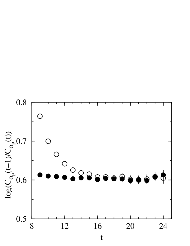
FIG. 1.: Effective mass plot with local source(open circles) and smeared source (solid circles) at $m_{Q}=2.6,\kappa=0.1585$ with the NRQCD action including entire $1/m_{Q}^{2}$ corrections (set II).

FIG. 2.: Effective plot of $C_{J_{P}}^{S(i)}(t)$ for pseudoscalar at $m_{Q}=2.6,\kappa=0.1585$ with set II. Where i=2,3,4,5 correspond to circles, squares, diamonds and triangles, respectively.

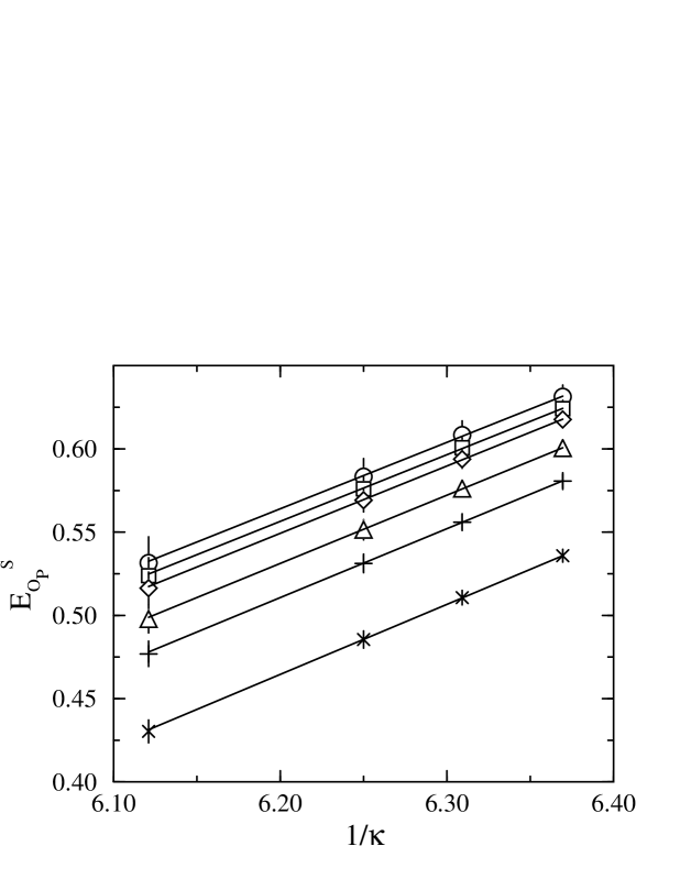
FIG. 3.: Chiral extrapolations of of $E_{{\cal O}_{P}}^{S}$. From above $am_{Q}$ = 5.0(circles), 2.6(squares), 2.1(diamonds), 1.5(triangles), 1.2(pluses) and 0.9(crosses) in set II.

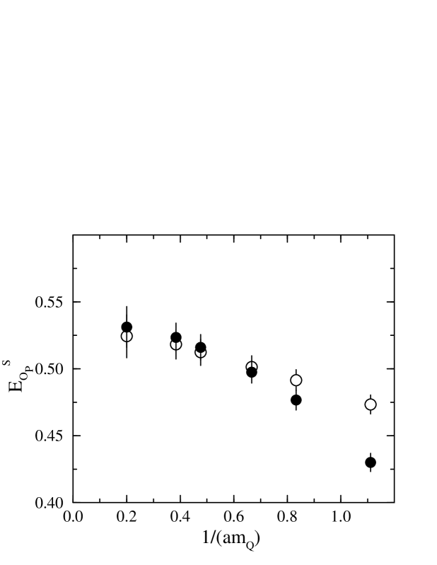
FIG. 4.: $1/(am_{Q})$ dependence of chirally extrapolated binding energies of pseudoscalar(circles) meson from set I(open) and set II(solid).

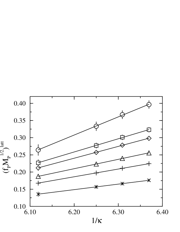
FIG. 5.: Chiral extrapolations of $(f_{P}M_{P}^{1/2})^{latt}$. From above $am_{Q}$ = 5.0(circles), 2.6(squares), 2.1(diamonds), 1.5(triangles), 1.2(pluses) and 0.9(crosses) in set II. Solid lines are obtained from linear fits.

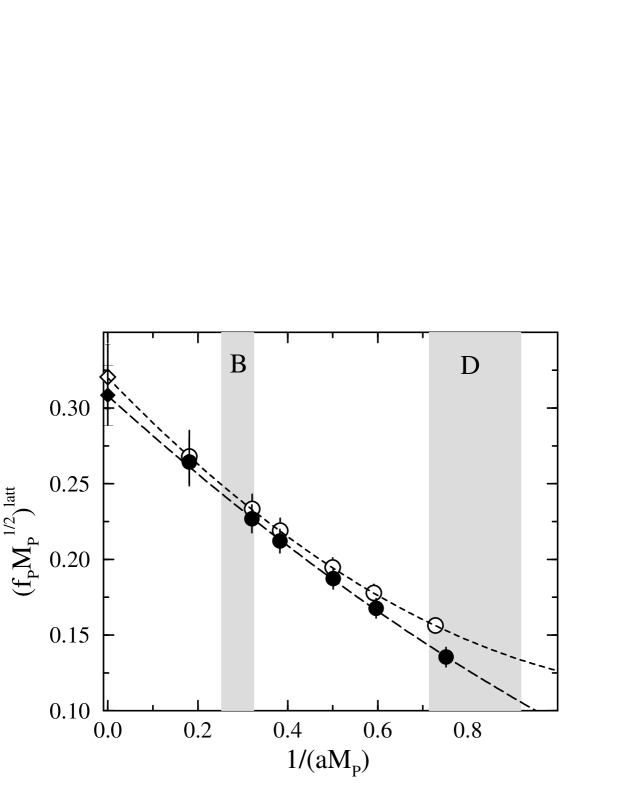
FIG. 6.: $1/(aM_{P})$ dependence of chirally extrapolated $(f_{P}M_{P}^{1/2})^{latt}$ with set I(open circles) and set II(solid circles). The dashed line is obtained by fitting the data from set I to quadratic function and the long dashed line from set II.

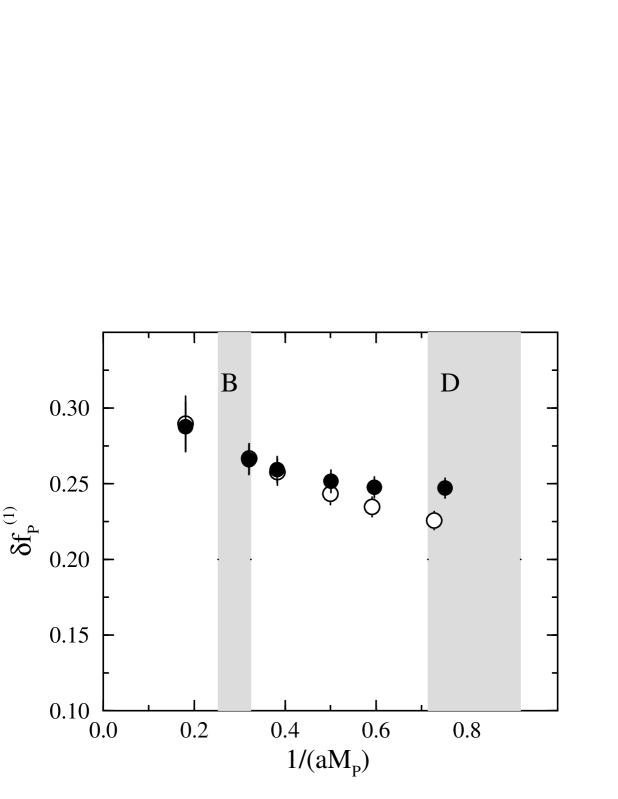
FIG. 7.: $1/(aM_{P})$ dependence of the leading contribution to $(f_{P}M_{P}^{1/2})^{latt}$ with set I(open circles) and set II(solid circles).

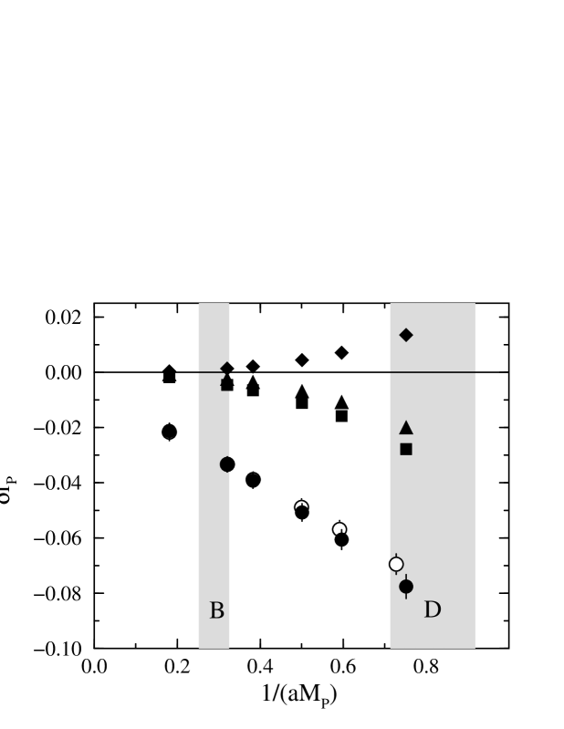
FIG. 8.: $1/(aM_{P})$ dependence of the non-leading contributions to $(f_{P}M_{P}^{1/2})^{latt}$ with set I(open circles) and set II(solid symbols). Solid symbols $\delta f_{P}^{(i)}$(i=2,3,4,5) are corresponding to circles, squares, diamonds and triangles respectively.

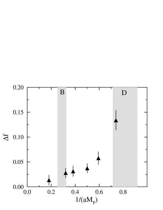
FIG. 9.: $1/(aM_{P})$ dependence of $O(1/m_{Q}^{2})$ correction.

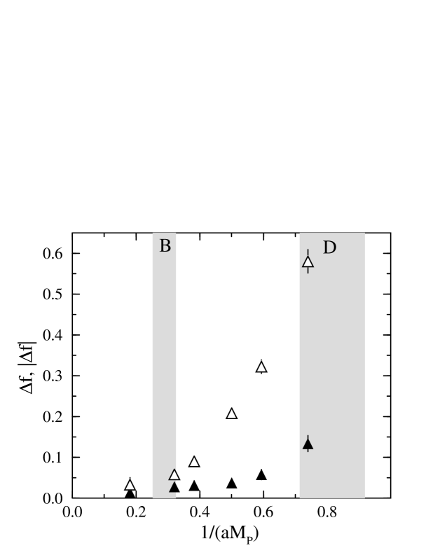
FIG. 10.: $1/(aM_{P})$ dependence of real $O(1/m_{Q}^{2})$ correction $\triangle f$(solid) and imaginary one $|\triangle f|$ (open). For detail, see text.

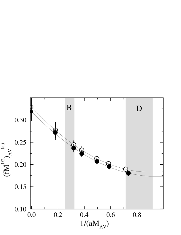
FIG. 11.: $1/(aM_{AV})$ dependence of spin averaged $(fM^{1/2})_{AV}^{latt}$ with set I(open circles) and set II(solid symbols). Solid line are obtained from a quadratic fit and Small symbols represent the extrapolated values.

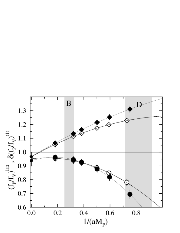
FIG. 12.: $1/(aM_{P})$ dependence of the ratio $(f_{P}/f_{V})^{latt}$ and $(f_{P}/f_{V})^{(1)}$ at $\kappa=\kappa_{c}$ with set I(open symbols) and set II(solid symbols). Circles refer to $(f_{P}/f_{V})^{latt}$, diamonds refer to $(f_{P}/f_{V})^{(1)}$.

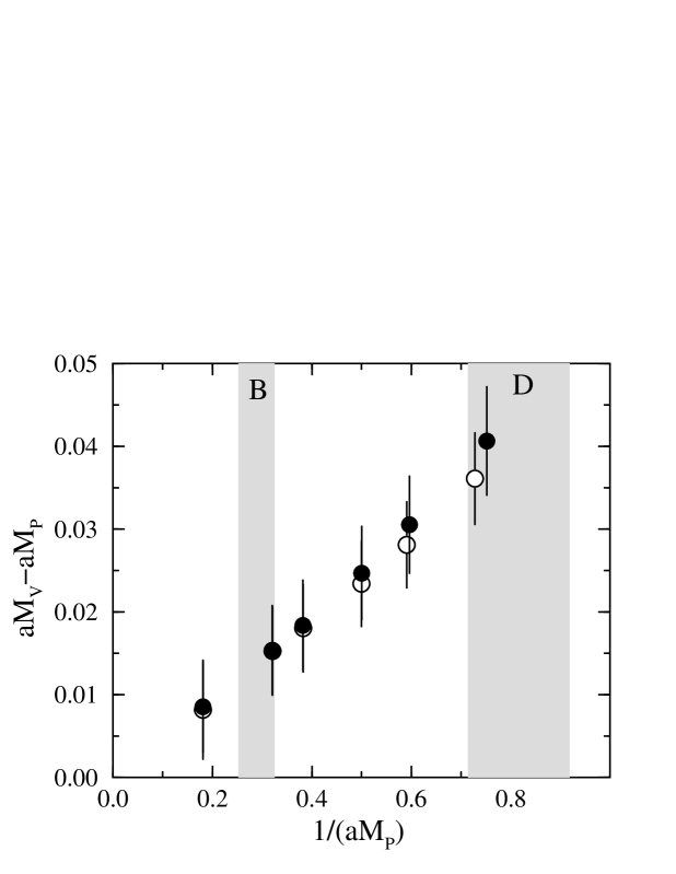
FIG. 13.: $1/(aM_{P})$ dependence of 1S hyperfine splitting with set I(open symbols) and set II(solid symbols).

FIG. 14.: $1/(aM_{P})$ dependence of $M_{P_{s}}-M_{P}$ with set I(open symbols) and set II(solid symbols).

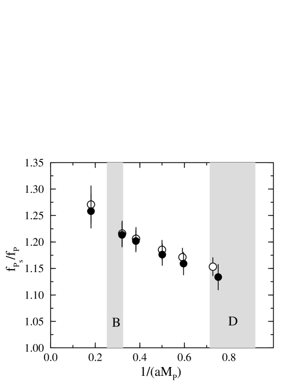
FIG. 15.: $1/(aM_{P})$ dependence of $f_{P_{s}}/f_{P}$ with set I(open symbols) and set II(solid symbols).

REFERENCES

- [1] Particle Data Group, Phys. Rev. D54, 1 (1996).
- [2] For a recent review see, for example, J. Flynn, Nucl. Phys. B (Proc. Suppl.) 53, 168 (1997).
- [3] B. A. Thacker and G. P. Lepage, Phys. Rev. D43, 196 (1991); G.P. Lepage, L. Magnea, C. Nakhleh, U. Magnea and K. Hornbostel, Phys. Rev. D46 4052 (1992).
- [4] UKQCD Collaboration, presented by C. T. H. Davies, Nucl. Phys. B (Proc. Suppl.)30, 437 (1993).
- [5] S. Hashimoto, Phys. Rev. D50, 4639 (1994).
- [6] S. Collins, U.M. Heller, J.H. Sloan, J. Shigemitsu, A. Ali Khan and C.T.H. Davies, Phys. Rev. D55, 1630 (1997); A. Ali Khan, J. Shigemitsu, S. Collins, C.T.H. Davies, C. Morningstar and J. Sloan, hep-lat/9704008.
- [7] A. Ali Khan, T. Bhattacharya et al., Nucl. Phys. B(Proc. Suppl.)53, 368 (1997).
- [8] G. P. Lepage and P. B. Mackenzie, Phys. Rev. D48, 2250 (1993).
- [9] G. P. Lepage, Nucl. Phys. B(Proc. Suppl.) 26, 45 (1992); A. X. El-Khadra, A. Kronfeld and P. Mackenzie, Phys. Rev. D55, 3933 (1997).
- [10] J. Shigemitsu, talk given at the International Workshop “Lattice QCD on Parallel Computers”, University of Tsukuba, Tsukuba, Japan, March 10-15 1997, to appear in Nucl. Phys. B(Proc. Suppl.), hep-lat/9705017.
- [11] C.T.H. Davies and B.A. Thacker, Phys. Rev. D45, 915 (1992); C.J. Morningstar, Phys. Rev. D48, 2265 (1993).
- [12] Ph. Boucaud, C.L. Lin and O. Pène, Phys. Rev. D40 1529 (1989) and Phys. Rev. D41 3541 (1990), E. Eichten and B. Hill, Phys. Lett. B240, 193 (1990).