Abelian Monopoles in $SU(2)$ Lattice Gauge Theory
as Physical Objects

Abstract

By numerical calculations we show that the abelian monopole currents are locally correlated with the density of the $SU(2)$ lattice action. This fact is established for the maximal abelian projection. Thus, in the maximal abelian projection, the monopoles are physical objects, they carry the $SU(2)$ action. Calculations on the asymmetric lattice show that the correlation between monopole currents and the density of the $SU(2)$ lattice action also exists in the deconfinement phase of gluodynamics.

I Introduction

The monopoles in the maximal abelian projection (MaA projection) of $SU(2)$ lattice gluodynamics [2] seem to be responsible for the formation of the flux tube between the test quark-antiquark pair. The $SU(2)$ string tension is well described by the contribution of the abelian monopole currents [3, 4, 5] which satisfy the London equation for a superconductor [6]. The study of monopole creation operators shows that the abelian monopoles are condensed [7, 8, 9] in the confinement phase of gluodynamics.

On the other hand, the abelian monopoles arise in the continuum theory [10] from the singular gauge transformation and it is not clear whether these monopoles are “real” objects. A physical object is something which carries action and in the present publication we only study the question if there are any correlations between abelian monopole currents and $SU(2)$ action. In [11] it was found that the total action of $SU(2)$ fields is correlated with the total length of the monopole currents, so there exists a global correlation. Below we discuss the local correlations between the action density and the monopole currents.

II Correlators of Monopole Currents and Density of $SU(2)$ Action

The simplest quantity which reflects the correlation of the local action density and the monopole current is the relative excess of $SU(2)$ action density in the region near the monopole current. It can be defined as follows. Consider the average action $S_{m}$ on the plaquettes closest to the monopole current $j_{\mu}(x)$. Then the relative excess of the action is

$$\eta=\frac{S_{m}-S}{S}\,,$$ (1)

where $S$ is the standard expectation value of the lattice action, $S=<\left(1-\frac{1}{2}Tr\,U_{P}\right)>$. $S_{m}$ is defined as follows:

$$S_{m}=<\frac{1}{6}\sum_{P\in\partial C_{\nu}(x)}\left(1-\frac{1}{2}Tr\,U_{P}\right)>\,,$$ (2)

where the average is implied over all cubes $C_{\nu}(x)$ dual to the magnetic monopole currents $j_{\nu}(x)$, the summation is over the plaquettes $P$ which are the faces of the cube $C_{\nu}(x)$; $U_{P}$ is the plaquette matrix. For the static monopole we have $j_{0}(x)\neq 0,\,j_{i}(x)=0,\,i=1,2,3$, and only magnetic part of $SU(2)$ action density contributes into $S_{m}$. The correlation of the monopole currents and the electric part of the action (which comes from more distant plaquettes) will be studied in another publication.

At large values of $\beta$, the quantity $\eta$ is equal to the normalized correlator of the dual action density and the monopole current:

$$C=\frac{<\frac{1}{2}Tr\,\left(j_{\mu}(x)\,\tilde{F}_{\mu\nu}(x)\right)^{2}>}{<j_{\mu}^{2}(x)><\frac{1}{2}TrF_{\alpha\beta}^{2}(x)>}-1\,.$$ (3)

Here the lattice regularization is implied, in particular,

$$\left<\frac{1}{2}TrF_{\alpha\beta}^{2}(x)\right>=\left<\left(1-\frac{1}{2}Tr\,U_{P}\right)\right>\,,$$

$$\left<\frac{1}{2}Tr\,\left(j_{\mu}(x)\,\tilde{F}_{\mu\nu}(x)\right)^{2}\right>=\left<\sum\limits^{4}_{\mu=1}j_{\mu}^{2}(x)\cdot\frac{1}{6}\sum\limits_{P\in\partial C_{\mu}(x)}\left(1-\frac{1}{2}Tr\,U_{P}\right)\right>\,,$$

the notations are the same as in (2). In the MaA projection at sufficiently large values of $\beta$, the probability of $j_{\mu}(x)=\pm 2$ is small. From the definitions (1), (2) and (3), it follows that if $j_{\mu}(x)=0,\pm 1$, then $\eta=C$. Numerical calculations show that $\eta=C$ with the accuracy of 5% for $\beta>1.5$ on lattices of sizes $10^{4}$ and $12^{3}\cdot 4$.

III Numerical Results

We calculate the quantities $\eta$ and $C$ on the symmetric $10^{4}$ lattice and on $12^{3}\cdot 4$ lattice which corresponds to finite temperature. In both cases, it occurs that in the MaA projection we have $\eta\neq 0$ and $C\neq 0$ for all values of $\beta$. We also consider the abelian projection which corresponds to the diagonalization of the plaquette matrices in the 12 plane (the $F_{12}$ gauge) and the diagonalization of the Polyakov line (the Polyakov gauge).

In Fig. 1 we show the dependence of the quantity $\eta$ on $\beta$ for $10^{4}$ lattice for the MaA projection and for the Polyakov gauge. It turns out that the data for the $F_{12}$ projection coincide within statistical errors with the data for the Polyakov gauge and we do not show these. In Fig. 3 we plot the same data, this time, for the $12^{3}\cdot 4$ lattice. It is seen that the quantity $\eta$ is much smaller for the Polyakov gauge than that for the MaA projection; the deconfinement phase transition at $\beta\approx 2.3$ does not have much influence on the behavior of $\eta$. Thus, the monopole currents in the MaA projection are surrounded by plaquettes which carry the values of $SU(2)$ action larger than the value of the average action.

To obtain these results we consider 24 statistically independent configurations of $SU(2)$ gauge fields for $\beta\leq 2.0$, 48 configurations for $2.25\leq\beta\leq 2.35$, and 120 configurations for $\beta\geq 2.4$. To fix the MaA projection we have used the overrelaxation algorithm [12]. The number of the gauge fixing iterations is determined by the criterion given in  [13]: the iterations are stopped when the matrix of the gauge transformation $\Omega(x)$ becomes close to the unit matrix: ${\rm max}_{x}\{1-{\frac{1}{2}}Tr\,\Omega(x)\}\leq 10^{-5}$. It has been checked that more accurate gauge fixing does not change our results.

The correlation of the currents and the action density can be explicitly visualized. In Fig. 3 we show the “time” slice of $10^{4}$ lattice. The monopole currents are represented by lines (or by large dots, if the current is perpendicular to the time slice). The monopole currents are obtained in the MaA projection from the gauge field configurations generated at $\beta=2.4$. The density of the small dots is proportional to $S(x)\,\theta\left(S(x)-S_{c}\right)$; the action density is defined as usual: $S(x)=\sum_{\mu\nu}\left(1-\frac{1}{2}Tr\,U_{\mu\nu}(x)\right)$. In Fig. 3 we have $S_{c}=0.75<S(x)>$. For this value of the threshold $S_{c}$, the correlation has been found to be most conspicuous. In Fig. 3 one can see some currents which are not surrounded by small dots. This indicates that near these currents we have $S(x)\leq S_{c}$. Moreover, there are some regions with high density of the action which are not related to the monopole currents. Inspecting several gauge field configurations, we have found that in most cases these regions are related to closed monopole currents in the neighboring time slice. At $\beta=2.4$, approximately 30% of the regions with high action density are not explicitly related to the monopole currents.

Thus we have found that, in the MaA projection, the abelian monopole currents and the regions with an excess of the nonabelian action density are spatially correlated. We conclude that the monopoles in the MaA projection carry action and thus constitute physical objects. It does not mean that these have to propagate in the Minkovsky space; a chain of instantons can produce a similar effect: an enhancement of the action density along a line in Euclidean space. It is important to understand what is the general class of configurations of $SU(2)$ fields which generate monopole currents. Some specific examples are known, in particular, the instantons [14, 15, 16, 17, 18] and the BPS–monopoles (periodic instantons) [19]. This question can be reformulated in another way: are there any continuum physical objects which correspond to abelian monopoles obtained in the MaA projection?

FIG. 1.: The relative excess of the magnetic action density near the monopole current, $\eta$, for the $10^{4}$ lattice. Circles correspond to MaA projection, squares correspond to Polyakov gauge.

FIG. 2.: The same as in Fig. 1, but for the asymmetric lattice $12^{3}\cdot 4$.

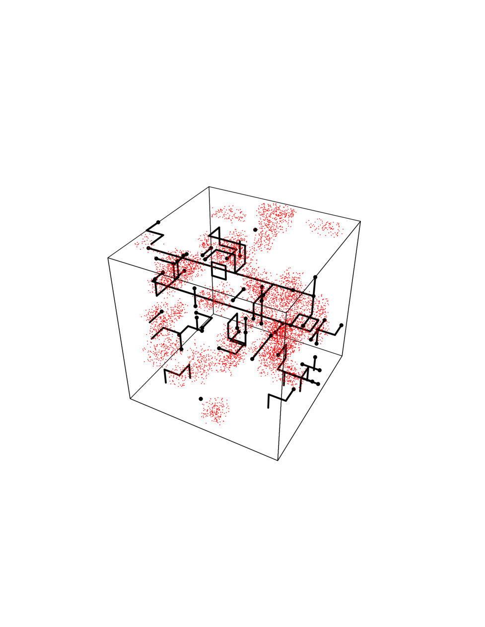
FIG. 3.: Three dimensional slice of the four dimensional $10^{4}$ lattice. The lines and the big dots mark the monopole currents, the density of the small dots is proportional to $SU(2)$ action density.

- [1] Also at Department of Physics, Kanazawa University, Kanazawa 920-11, Japan
- [2] A.S. Kronfeld, M.L. Laursen, G. Schierholz and U.J. Wiese, Phys. Lett.198B, 516 (1987); A.S. Kronfeld, G. Schierholz and U.J. Wiese, Nucl. Phys.B293, 461 (1987).
- [3] H. Shiba and T. Suzuki, Phys. Lett.B333, 461 (1994).
- [4] J.D. Stack, S.D. Neiman and R.J. Wensley, Phys. Rev. D 50, 3399 (1994).
- [5] G.S. Bali, V. Bornyakov, M. Mueller-Preussker, K. Schilling; Phys. Rev. D 54, 2863 (1996).
- [6] V. Singh, D. Browne and R. Haymaker, Phys. Lett.B306 115 (1993).
- [7] L. Del Debbio, A. Di Giacomo, G. Paffuti and P. Pieri, Phys. Lett.B355, 255 (1995).
- [8] N. Nakamura et all., Nucl. Phys. Proc. Suppl. 53, 512 (1997).
- [9] M.N. Chernodub, M.I. Polikarpov and A.I. Veselov, Phys. Lett.B399, 267 (1997).
- [10] G. ’t Hooft, Phys. Lett.B190 [FS3], 455 (1981).
- [11] H. Shiba and T. Suzuki, Phys. Lett.B351, 519 (1995).
- [12] J.E. Mandula and M. Ogilvie, Phys. Lett.248B, 156 (1990).
- [13] V.G. Bornyakov et al., Phys. Lett.B261, 116 (1991); G.I. Poulis, Phys. Rev. D 56, 161 (1997).
- [14] M.N. Chernodub and F.V. Gubarev, Pis’ma Zh. Eksp. Teor. Fiz. 62, 91 (1995) [JETP Lett. 62, 100 (1995)].
- [15] A. Hart and M. Teper, Phys. Lett.B371, 261 (1996).
- [16] H. Suganuma et all., Aust. J. Phys. 50, 233 (1997).
- [17] R.C. Brower, K.N. Orginos and Chung-I Tan, Phys. Rev. D 55, 6313 (1997).
- [18] M. Feurstein, H. Markum and S. Thurner, Phys. Lett.B396, 203 (1997).
- [19] J. Smit and A. van der Sijs, Nucl. Phys.B355, 603 (1991).