Abstract

Using the geometric definition of the topological charge we decompose the path integral of 2-dimensional U(1) lattice gauge theory into topological sectors. In a Monte Carlo simulation we compute the average value of the action as well as the distribution of its values for each sector separately. These numbers are compared with analytic lower bounds of the action which are relevant for classical configurations carrying topological charge. We find that quantum fluctuations entirely dominate the path integral. Our results for the probability distribution of the Monte Carlo generated configurations among the topological sectors can be understood by a semi-phenomenological argument.

 

^∗ Supported by Fonds zur Förderung der Wissenschaftlichen Forschung in Österreich, Projects P11502-PHY and J01185-PHY.

The last few years have seen an ever increasing interest in studying topological ideas in lattice gauge theories (see [3] for a recent review). Many of these studies were motivated by computing statistical properties of instantons such as their average size and density distribution which are of interest for semiclassical models [4] (see [5] for an analysis of these ideas for the case of gauge group U(1) and 2 dimensions). Rather than using the lattice to extract information on some underlying classical configurations, in a series of articles [6] we directly investigate possible implications of the existence of a topological structure for the lattice path integral.

Here we study the characteristic values for the action of quantum fluctuations and compare them to analytic lower bounds of the action in each topological sector. Classical configurations carrying topological charge typically have action in the vicinity of these bounds. It is interesting to analyze whether after adding quantum fluctuations the structure of the classical configurations is still relevant for the physical picture.

The model under consideration is U(1) lattice gauge theory in 2 dimensions. Due to the simplicity of this model good statistics is easy to obtain. The model has the further advantage of possessing a simple form of the topological charge; the geometric definition based on Lüscher’s work [7] can be computed easily without making use of sophisticated techniques such as cooling or analyzing the spectrum of the Dirac operator. These two facts allow to explore the physical mechanisms governing the role of topology on the lattice in a rather playful way.

Before we start developing our results we find it useful to comment on the relevance of topological arguments in the continuum and on the lattice. In the continuum it is possible to classify classical, i.e. differentiable configurations with respect to their topological charge. It is crucial to note that these classical configurations are of measure zero in the continuum path integral [8]. Thus in the continuum topological arguments cannot go beyond a semiclassical analysis. On the lattice the situation is different. In particular for the case of U(1)₂ lattice gauge theory one can assign a topological charge to all configurations (except for so-called exceptional configurations which are of measure zero). For SU(N)₄ it is believed, that the path integral in the continuum limit is dominated by smooth configurations which also can be assigned a topological charge. Thus in a certain sense, the lattice formulation is more powerful for studying topological ideas and the lattice path integral can indeed be decomposed into topological sectors. In particular the outlined questions can be formulated in a meaningful way and a consistent physical picture can be obtained.

We work on a 2-dimensional square lattice $\Lambda$ with length $L$. Lattice sites are denoted as $x=(x_{1},x_{2})$ with $x_{i}=1,2,...,L$. The lattice spacing is set equal to 1. The gauge fields are group elements $U_{\mu}(x)\in\mbox{U(1)}$ assigned to the links between nearest neighbours $x,x+\hat{\mu}$ and their action is given by

$$S\;=\;\beta\sum_{x\in\Lambda}\;\Big{[}\;1\;-\;\mbox{Re}\;U_{P}(x)\;\Big{]}\;.$$ (1)

The plaquette element is defined as $U_{P}(x)=U_{1}(x)U_{2}(x+\hat{1})\overline{U_{1}(x+\hat{2})}\;\overline{U_{2}(x)}$. The gauge fields obey periodic boundary conditions $U_{\mu}(L+1,x_{2})=U_{\mu}(1,x_{2})$, $U_{\mu}(x_{1},L+1)=U_{\mu}(x_{1},1)$.

The model was simulated with the hybrid Monte Carlo algorithm[9] (this calculation is part of a another project including also fermions [6]) with 10-step trajectories adjusted such that the acceptance rate in the Monte Carlo step was 0.8 in the mean. For all lattices sizes (up to $16\times 16$) we averaged $10^{5}$ measurements. The individual measurements have been separated by 10 updates (for small values of $\beta$) up to 500 updates (for $\beta=6$) in order to reduce correlations.

To check our algorithm we compare our results for simple observables such as $\langle S/L^{2}\rangle$ with the outcome of the analytic solution for the model with open boundary conditions (see e.g. [10]). We find excellent agreement (within the small statistical errors), and only for the $L=4$ lattice we observed small deviations due to the different boundary conditions.

For the computation of the topological charge we use the geometric definition which is based on Lüscher’s idea of associating a principal bundle to each lattice configuration and defining its topological charge through the topological charge of the bundle [7]. The case of QED₂ was worked out in [11]. One obtains

$$\nu[U]\;=\;\frac{1}{2\pi}\sum_{x\in\Lambda}\theta_{P}(x)\;,$$ (2)

where the plaquette angle $\theta_{P}(x)$ is given by $\theta_{P}(x)=-i\ln U_{P}(x)$ and restricted to the principal branch $\theta_{P}(x)\in(-\pi,\pi)$. Note that configurations where $U_{P}(x)=-1$ for some $x$ are so-called exceptional configurations and Lüscher’s definition does not assign a value $\nu[U]$ to them. Those configurations are of measure zero in the path integral.

An interesting observable [12, 13] is the probability distribution of the Monte Carlo generated configurations among the topological sectors. In Fig. 1 we show our results for a $16\times 16$ lattice and $\beta=4$ and 6. For both values of $\beta$ we observe a symmetric, Gaussian-like distribution centered at $\nu=0$. It becomes more peaked with increasing $\beta$.

Figure 1: Probability distribution $p(\nu)$ of Monte Carlo generated configurations among the topological sectors. The symbols give our results from a $16\times 16$ lattice for $\beta=4$ and $6$ ($10^{5}$ configurations each), the curve is the semi-phenomenological distribution function (6).

Naturally the following question arises: What is the mechanism behind this distribution of Monte Carlo configurations among the topological sectors? A first guess is, that there is a lower bound for the gauge field action in each topological sector. Such a bound would force the action to higher values when increasing $|\nu|$ and through the Boltzmann factor lead to a suppression of configurations in higher sectors.

Here we use two different lower bounds, a strict bound and a bound which holds only for sufficiently large $\beta$ but is more interesting from a physical point of view. The first one resembles the famous result [14] for classical Yang-Mills configurations in 4 dimensions. It also can be derived using the Schwartz inequality [15]. Essentially the same arguments can be repeated on the lattice. We assume that the lattice gauge configuration $U$ is non-exceptional such that a topological charge (2) can be assigned. We use the Schwartz inequality to obtain

$$\left|\sum_{x\in\Lambda}\theta_{P}(x)\right|^{2}\!=\left|\sum_{x\in\Lambda}\frac{\theta_{P}(x)}{1\!-\!e^{i\theta_{P}(x)}}[1\!-\!e^{i\theta_{P}(x)}]\right|^{2}\!\leq\sum_{x\in\Lambda}[1\!-\cos\theta_{\!P}(x)]\times\!\sum_{y\in\Lambda}\frac{\theta_{P}(y)^{2}}{1\!-\!\cos\theta_{\!P}(y)}.$$

Using (1) and (2) one ends up with

$$S[U]\;\;\;\geq\;\;\;\frac{2\pi^{2}}{L^{2}}\beta\;\Big{|}\nu[A]\Big{|}^{2}\;D[U]\;\;\;\geq\;\;\;\frac{2\pi^{2}}{L^{2}}\beta\;\Big{|}\nu[A]\Big{|}^{2}\;\frac{4}{\pi^{2}}\;,$$ (3)

where

$$\frac{4}{\pi^{2}}\;\;\leq\;\;D[U]\;=\;2\left[\frac{1}{L^{2}}\sum_{x\in\Lambda}\frac{\theta_{P}(x)^{2}}{1-\cos\theta_{P}(x)}\right]^{-1}\;\;\leq\;\;1\;.$$ (4)

$D[U]$ is a measure for how much the average plaquette angle differs from $0$. This functional takes values between $4/\pi^{2}$ and 1. In the latter case which corresponds to $\beta\rightarrow\infty$, (3) equals the bound valid for classical configurations on a continuous 2-dimensional compact manifold (replace $L^{2}$ by the volume of the manifold).

Another formula also serves as a lower bound for sufficiently smooth configurations and is more stringent. Using the fact that the function $(1-\cos\theta)$ (the contribution of one plaquette to the gauge field action) is convex for $|\theta|\leq\pi/2$ one finds

$$\frac{1}{L^{2}}\sum_{x\in\Lambda}\;[\;1-\cos\theta_{P}(x)\;]\;\;\geq\;\;1-\cos\left(\frac{1}{L^{2}}\sum_{x\in\Lambda}\theta_{P}(x)\right)\;,$$

which implies

$$S[U]\;\;\geq\;\;\beta L^{2}\Big{[}1-\cos\Big{(}\frac{2\pi}{L^{2}}\nu[U]\Big{)}\Big{]}\;.$$ (5)

It has to be stressed, that this bound holds only if for all $x\in\Lambda$ the condition $|\theta_{P}(x)|\leq\pi/2$ is fulfilled. However for large enough $\beta$ this is the case and (5) holds. For small $|\nu|$ it is more stringent than the exact bound (3) (compare Table 1).

It is interesting to note, that the right hand side of (5) is the value of the lattice action (1) for configurations which correspond to continuum fields with constant electric field $2\pi\nu/V$, where $V$ is the volume of the base manifold. In [16] the path integral for the Schwinger model an a continuous torus was constructed essentially using those constant field configurations and adding quantum fluctuations. The lower bound (5) is thus of particular interest for analyzing the emergence of the physical picture in the continuum [5, 16] from a lattice formulation.

parameters	$\nu$	$\overline{S}(\nu)/L^{2}$	$\overline{S}_{ph}(\nu)/L^{2}$	bound (3)	bound (5)
$L=8$	0	0.536(5)	0.536	0	0
$\beta=4$	1	0.556(8)	0.553	0.0078	0.0193
	2	0.62(4)	0.603	0.0312	0.0768
$L=16$	0	0.543(3)	0.543	0	0
$\beta=4$	1	0.545(3)	0.544	0.0004	0.0012
	2	0.549(4)	0.547	0.0019	0.0048
	3	0.555(9)	0.552	0.0044	0.0108
$L=16$	0	0.523(3)	0.523	0	0
$\beta=6$	1	0.525(3)	0.525	0.0007	0.0018
	2	0.530(6)	0.530	0.0029	0.0072
	3	0.540(16)	0.538	0.0066	0.0163

Table 1: Data for the action in various topological sectors. For several values of $L,\beta$ and $\nu$ we give the average value of the action per plaquette $\overline{S}(\nu)/L^{2}$ the phenomenological value $\overline{S}_{ph}(\nu)/L^{2}$ from (7) and the values for the lower bounds (3) and (5) (also normalized with $L^{-2}$).

In order to study the outlined idea that lower bounds of the action in each sector are responsible for the distribution in Fig. 1, we compute the average value $\overline{S}(\nu)/L^{2}$ of the action for each topological sector separately and compare this average with the values of the lower bounds (3) and (5). Fig. 2 and Table 1 give our results.

Figure 2: Average value $\overline{S}(\nu)/L^{2}$ of the action per plaquette in various topological sectors. The symbols are the results of our Monte-Carlo simulation, the horizontal lines are the values from the analytic solution for open boundary conditions $[7]$. The curves connecting the symbols come from the semi-phenomenological formula (7) to be discussed below. We show our results for $L=8,16$ and $\beta=2$ (circles), $\beta=4$ (squares) and $\beta=6$ (diamonds).

In the figure the symbols show the average value of the action per plaquette and the horizontal lines give the value of the analytic result for open boundary conditions [10] which is a sum over all sectors. The curve connecting the symbols comes from the phenomenological formula (6) below. The average value of the action increases with increasing values of $|\nu|$ and thus the distribution of Fig. 1 can be understood through the suppression by the Boltzmann factor.

What is indeed surprising is the fact, that the values of the analytic lower bounds (3) and (5) are far below the actual average values of the action in the path integral (see Table 1). For all sectors the action stays close to the analytic value [10] which is a sum over all sectors (horizontal lines). Only the center of the distribution slightly dips below this value. The range of values for the analytic lower bounds (and thus the action for the constant field configurations [16]) is typically one order of magnitude smaller (see Table 1).

To study the quantum fluctuations further we analyze the distribution of the values of the action in a fixed sector. It can be computed by binning the range of values of the action and counting the number of configurations in each bin. In Fig. 3 we show histograms for the probability distribution of the action per plaquette in the sectors with $\nu=0,1$ and 2. The vertical lines show the average value $\overline{S}(\nu)$ of the action in each sector as well as the lower bound (5).

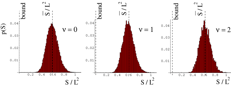
Figure 3: Probability distribution $p(S)$ of the action per plaquette in the sectors $\nu=0,1,2$. The data was taken on a $8\times 8$ lattice at $\beta=2$. The dotted vertical lines indicate the value of the lower bound $(5)$ and the average $\overline{S}(\nu)/L^{2}$ for each sector.

It is obvious, that quantum fluctuations keep a large portion of the configurations high above the lower bounds (3) and (5). For all sectors the configurations have action close to the value given by the analytic solution [10] for open boundary conditions. Comparison with the lower bound (5) which gives the characteristic action for classical, topologically non-trivial configurations shows the importance of quantum fluctuations. This dominance of the quantum fluctuations was already conjectured in a study of the model on the continuous torus [5]. We remark that we obtain similar distributions for other values of $L$ and $\beta$. For increasing $L$ the total action of the configurations tends to be more concentrated around the peak, and the whole distribution is narrower, as expected. The lower bounds become even less important. Increasing $\beta$ makes the distribution less symmetric by increasing the weight of smaller values of the action, essentially without altering the support of the distribution.

Although the analytic lower bounds do not seem to govern the distribution of the values of the action in the fully quantized theory, it is still possible to use topological arguments in a phenomenological way to understand the distributions in Fig. 2. From the definition of the topological charge (2) it follows that the average increase of the plaquette angle when increasing $|\nu|$ by 1 is given by $2\pi/L^{2}$. Assuming that the effect of going from the trivial sector to a nontrivial sector can be taken into account by adding this average value to all plaquette angles one finds ($\theta^{0}_{P}(x)$ are the plaquette angles of a configuration in the trivial sector)

$$S_{ph}(\nu)=\beta\sum_{x\in\Lambda}\Big{[}1-\cos\Big{(}\theta^{0}_{P}(x)+\nu\frac{2\pi}{L^{2}}\Big{)}\Big{]}\;=$$

$$S(0)+\frac{2\,\pi\,\beta\,\nu}{L^{2}}\sum_{x\in\Lambda}\sin\theta^{0}_{P}(x)+\frac{2\,\pi^{2}\,\nu^{2}}{L^{4}}\left[-S(0)+\beta L^{2}\right]+O(\nu^{4}/L^{6})\;.$$

In the second step we assumed that $|\nu|$ is small compared to $L^{2}$, and expanded the cosine in $\nu/L^{2}$. The second order term has been re-expressed in terms of the total action.

The sum over $\sin\theta^{0}_{P}(x)$ may be neglected for two reasons. On one hand in the sum over all configurations it vanishes due to the symmetry of the Wilson action in the plaquette angle. Furthermore (at least in order $\theta^{0}_{P}(x)$) it is proportional to the topological charge which is zero per ansatz. We end up with the following formula for the average value of the action

$$\overline{S}_{ph}(\nu)\;=\;\overline{S}(0)+\nu^{2}\frac{2\pi^{2}}{L^{4}}\Big{[}-\overline{S}(0)+\beta L^{2}\Big{]}+O(\nu^{4}/L^{6})\;.$$ (6)

In Table 1 we give the values of (6) for the corresponding $\beta,L$ and $\nu$. The curves in Fig. 2 were drawn using (6). The formula gives reasonable values for the average action over a wide range of $\beta,L$ and $\nu$ with a slight tendency to underestimate the Monte Carlo results for smaller $\beta$. This tendency can be understood by the fact that $2\pi/L^{2}$ only gives the minimal increase of the average plaquette angle compatible with an increase of $|\nu|$ by 1. Quantum fluctuations seem to lead to slightly higher values of the average plaquette angle and thus of the action. When increasing $\beta$ the fluctuations are more suppressed and the quality of (6) increases.

We finally remark, that (6) can be used to understand the shape of the distribution in Fig. 1 and to test the ergodicity of the updating algorithm. Raising (6) to the exponent and normalizing the result gives the Gaussian distribution

$$p(\nu)=N\exp\left(-\frac{1}{2}\,C\,\nu^{2}\right)\;,\quad C=\frac{4\,\pi^{2}}{L^{4}}\left[-\overline{S}(0)+\beta\,L^{2}\right]\;,$$ (7)

with normalization (note that $\nu$ is an integer) $N^{-1}=\sum_{\nu}\exp(-\nu^{2}\,C/2)$. It should reproduce the probability distribution of the configurations among the topological sectors. The dotted lines in Fig. 1 show the Gaussian (8), and we find good agreement with the Monte Carlo data. The quality increases with $\beta$ and $L$ where formulas (6) and (7) are more reliable. Thus the probability distribution of Fig. 1 can indeed be understood using topological arguments. We conclude that our updating algorithm is ergodic.

Using a different definition of the topological charge, Bardeen et al. [13] derive a similar formula for $p(\nu)$ from the analytic solution [10]. In the limit $\beta\rightarrow\infty$, where the two definitions of the topological charge are expected to coincide, their result approaches our formula (7). In fact, replacing $\overline{S}(0)$ in (6) by the analytic result for infinite lattices, proportional to $[1-I_{1}(\beta)/I_{0}(\beta)]$ (which, however, sums all topological sectors) one recovers the distribution given in [13].

The most remarkable outcome of this study is the fact, that quantum fluctuations entirely dominate the path integral. At the values of $L$ and $\beta$ where our simulations were performed, the configurations which essentially contribute to the path integral have values of the action which are typically one order of magnitude larger than the analytic lower bounds. This dominance of quantum fluctuations was already conjectured for the model on the continuous torus in [5]. In the underlying construction [16] the path integral is essentially decomposed into constant field configurations that carry topological charge and saturate the lower bound of the action, plus a field describing the quantum fluctuations. The observed importance of the quantum fluctuations shows that trying to establish a physical picture where dominant classical configurations are used to understand the interplay of topological charge and vacuum expectation values is questionable.

Using a semi-phenomenological ansatz we were able to obtain a qualitative, and in the $\beta\rightarrow\infty$ limit even quantitative understanding of the average behaviour of the action. This formula explains the probability distribution of Fig. 1 in terms of a topological argument and can be used to check the ergodicity of the updating algorithm.

We believe, that although the technical problems are much more severe, a similar study can – in principle – also be accomplished for lattice Yang Mills theory in 4 dimensions. The possible outcome would be a better understanding of the relation between quantum fluctuations and classical configurations carrying topological information.

We thank Philippe de Forcrand and Helmut Gausterer for interesting discussions. C.R. G. has also profited from remarks by Erhard Seiler and Gordon Semenoff.

References

- [1]
- [2]
- [3] A. Di Giacomo, Nucl. Phys. (Proc. Suppl.) B47 (1996) 136.
- [4] T. Schäfer and E. V. Shuryak, preprint hep-ph/9610451 (second version from April 18, 1997).
- [5] A. V. Smilga, Phys. Rev. D46 (1992) 5598; Phys. Rev. D49 (1994) 5480.
- [6] C. R. Gattringer, I. Hip and C. B. Lang, work in preparation.
- [7] M. Lüscher, Commun. Math. Phys. 85 (1982) 39.
- [8] P. Colella and O. E. Lanford III, in: Constructive Quantum Field Theory (Erice 73), G. Velo and A. Wightman (Eds.), Springer Lecture Notes in Physics, Springer 1973, New York.
- [9] S. Duane, A. D. Kennedy, B. J. Pendleton and D. Roweth, Phys. Lett. 195B (1987) 216.
- [10] J. Zinn-Justin, Quantum Field Theory and Critical Phenomena (Third Edition), Clarendon Press 1996, Oxford.
- [11] R. Flume and D. Wyler, Phys. Lett. 108B (1981) 317; C. Panagiotakopoulos, Nucl. Phys. B251 (1985) 61; A. Phillips, Ann. Phys. 161 (1985) 399; M. Göckeler, A. S. Kronfeld, G. Schierholz and U.-J. Wiese, Nucl. Phys. B404 (1993) 839; H. Gausterer and M. Sammer, preprint hep-lat/9609032.
- [12] Ph. de Forcrand, Margarita García Pérez and I.-O. Stamatescu, preprint hep-lat/9701012; R. Narayanan and P. Vranas, preprint hep-lat/9702005; B. Berg and M. Lüscher, Nucl. Phys. B190 (1981) 412.
- [13] W. Bardeen, A. Duncan, E. Eichten and H. Thacker, preprint hep-lat/9705002.
- [14] A. A. Belavin, A. M. Polyakov, A. S. Schwartz and Yu. S. Tyupkin, Phys. Lett. 59B (1975) 85.
- [15] R. Rajaraman, An Introduction to Solitons and Instantons in Quantum Field Theory, North Holland 1982, Amsterdam.
- [16] H. Joos, Helv. Phys. Acta 63 (1990) 670; I. Sachs and A. Wipf, Helv. Phys. Acta 65 (1992) 652.