CERN–TH/97–107 May 1997 O($a$) improved lattice QCD

Abstract

We review the O($a$) improvement of lattice QCD with special emphasis on the motivation for performing the improvement programme non-perturbatively and the general concepts of on-shell improvement. The present status of the calculations of various improvement coefficients (perturbative and non-perturbative) is reviewed, as well as the computation of the isospin current normalization constants $Z_{\rm A}$ and $Z_{\rm V}$. We comment on recent results for hadronic observables obtained in the improved theory.

1 INTRODUCTION

The leading cutoff effects in lattice QCD with Wilson quarks [1] are proportional to the lattice spacing $a$ and can be rather large for typical values of the Monte Carlo (MC) simulation parameters [2, 3]. Decreasing the lattice spacing at constant physical length scales means larger lattices and therefore rapidly increasing costs of the MC simulations.

An alternative method to reduce cutoff effects in lattice field theories is due to Symanzik [4, 5]. He has shown that the approach of Green’s functions to their continuum limit can be accelerated by using an improved action and improved (composite) fields. A considerable simplification is achieved if the improved continuum approach is only required for on-shell quantities such as particle masses and matrix elements of improved fields between physical states [6, 7].

Symanzik improvement may be viewed as an extension of the renormalization programme to the level of irrelevant operators. While the structure of the possible counterterms is dictated by the symmetries, their coefficients have to be fixed by appropriate improvement conditions. Although they can be estimated in (tadpole-improved [8]) perturbation theory, a non-perturbative determination of the improvement coefficients through MC simulations is clearly preferable.

To O($a$), we have recently carried out the non-perturbative improvement programme in quenched lattice QCD, thus leaving residual cutoff effects of O($a^{2}$) only. The details of the calculations are given elsewhere [9]–[13]. In this report we emphasize the general concepts and give a short account of the main results. We also discuss progress that is currently made in applying the improvement programme to full QCD with $N_{\rm f}=2$ flavours [14].

We start by outlining the importance of removing the linear (in $a$) lattice artefacts non-perturbatively (sect. 2). We then review on-shell improvement in the framework of Symanzik’s local effective theory (sect. 3) and the general concept of non-perturbative improvement (sect. 4). The practical calculations are done in finite space-time volume with Schrödinger functional boundary conditions which we introduce in sect. 5. We then review the computations of the various improvement coefficients and the current normalization constants in quenched lattice QCD. Residual lattice artefacts are discussed in sect. 9 and the status of ${\rm O}(a)$ improvement in full QCD in sect. 10.

2 WHY NON-PERTURBATIVE ${\rm O}(a)$ IMPROVEMENT?

In this workshop two main alternative approaches to reducing the cutoff effects of lattice QCD are discussed [15, 16]. Before giving some detailed motivation for what is discussed here, let us point out the relation to these talks. The goal of the perfect action approach [15] is the improvement of the lattice theory to all orders of the lattice spacing. In determining the perfect action, one – in practice – performs an expansion in powers of the coupling constant. In contrast, the non-perturbative Symanzik improvement as discussed here proceeds non-perturbatively in the coupling and order by order in the lattice spacing. On the other hand, “mean field improvement” [16] is Symanzik improvement with improvement coefficients approximated by mean field-improved perturbation theory [8].

Let us explain in more detail the motivation for non-perturbatively removing the lattice artefacts that are linear in $a$. The first motivation is that these are large numerically. We give two examples to illustrate this point.

The first example is a perturbative one. Consider the renormalized coupling $\bar{g}(L)$ defined in the Schrödinger functional scheme [17, 21, 19] for massless fermions. Its evolution from length scale $L$ to scale $2L$ defines the step scaling function $\Sigma$ [17, 18]. The one-loop contribution of $N_{\rm f}$ Wilson fermions to $\Sigma$ has been calculated in ref. [19]. We denote it by $\bar{g}^{4}N_{\rm f}\Sigma_{1,1}$ . Its continuum limit is given by the fermion contribution to the lowest term in the $\beta$-function:

$$\lim_{a/L\rightarrow 0}{\Sigma_{1,1}(L/a)\over\bar{g}^{4}N_{\rm f}}=2b_{0,1}\log(2)\,,\quad$$ (1)

$$b_{0,1}=-{1\over 24\pi^{2}}\,.$$

Without ${\rm O}(a)$-improvement, $\Sigma_{1,1}$ depends very strongly on $a/L$ and shows a smooth approach to the continuum only for very large lattices (cf. fig. 1). If one had MC data with $L/a\leq 10$ and such an error term, a naive continuum extrapolation of such data would overestimate the fermion contribution by O(60%). On the other hand, after ${\rm O}(a)$-improvement the lattice artefacts in this quantity are tiny.

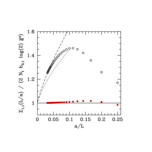
Figure 1: One-loop contribution of a massless Wilson quark to the step scaling function $\Sigma$ normalized to its continuum value. Open circles are for the Wilson action. The dotted curve describes the leading lattice artefact for small $a/L$, which is of the form $\log(a/L)a/L$, while the dashed curve contains the pure $a/L$-term in addition. Filled circles illustrate the behaviour after ${\rm O}(a)$-improvement.

The second example is the current quark mass $m$ defined by the PCAC relation. As we will discuss in detail below, its value is independent of kinematical variables such as the boundary conditions. Dependences on such variables are pure lattice artefacts. We examined the current quark mass in the valence approximation by numerical Monte Carlo simulations and found [2] large lattice artefacts even for quite small lattice spacings (cf. fig. 2).

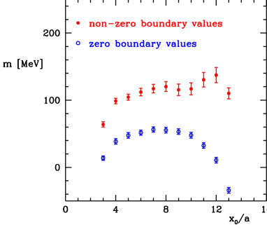
Figure 2: Dependence of curent quark mass $m$ on the boundary condition and the time coordinate. The calculation is done on a $16\times 8$ lattice at $\beta=6.4$, which corresponds to a lattice spacing of $a\approx 0.05\,{\rm fm}$. “Boundary values” refer to the gauge field boundary conditions in the SF [2]; see sects. 5,6 for details.

Since lattice artefacts can be large numerically, it is desirable to remove them non-perturbatively in order not to leave over $\alpha_{s}^{2}a$ or truly non-perturbative terms that may be noticeable.

A second motivation for performing improvement non-perturbatively is closely related. After improvement one wants to compute physical quantities $P$, such as ratios of hadron masses for a range of lattice spacings and extrapolate them to the continuum limit.

For example, assume that MC results $P(a)$ are available for four points $a^{2}=a_{0}^{2},\hbox{$3\over 4$}a_{0}^{2},\hbox{$1\over 2$}a_{0}^{2},\hbox{$1\over 4$}a_{0}^{2}$ and with statistical errors $\Delta P=\Delta$ that are independent of $a$. An extrapolation by means of a fit $P(a)=P_{\rm c}+s_{2}a^{2}$ will yield an estimate for the continuum limit of $P$ with error $\Delta P_{\rm c}=1.22\Delta$. However, if the calculation was performed with approximate values of the improvement coefficients, a small (?) linear error term $b\times a$ will be left in the results $P(a)$. If ignored, it causes a systematic error of size $0.35\,b\,a_{0}$ in $P_{\rm c}$. As an alternative, one may, of course, perform a fit with the ansatz $P(a)=P_{\rm c}+s_{1}a+s_{2}a^{2}$. This gives a continuum value with statistical error $\Delta P_{\rm c}=9.7\Delta$.

Trivial as it is, the above example illustrates the important point: in order to perform a reliable continuum extrapolation, one must have theoretical information on the expected $a$-dependence. This is contained in the structure of Symanzik’s effective action, which justifies a power series in the lattice spacing for the correction terms. (For the purpose of extrapolating MC-data, the logarithmic dependence on $a$ can be ignored). Under the same assumption, namely that lattice artefacts higher than $a^{2}$ can be neglected, the continuum extrapolation in the ${\rm O}(a)$-improved theory gives errors that are smaller by a factor 8 than the extrapolation in the unimproved (or approximately improved) case.

Natural as it may seem to continue the non-perturbative Symanzik improvement beyond the first order in the lattice spacing, this appears impossible in practice. The reason is that at order O($a^{2}$) a large number of improvement terms would have to be determined by MC calculations.

3 ON-SHELL IMPROVEMENT

3.1 Lattice QCD with Wilson quarks

In this section we consider QCD on an infinitely extended lattice with two degenerate light Wilson quarks of bare mass $m_{0}$ [1]. The action is the sum of the usual Wilson plaquette action and the quark action

$$S_{\rm F}[U,\overline{\psi},\psi\,]=a^{4}\sum_{x}\overline{\psi}(x)(D+m_{0})\psi(x),$$ (2)

where $a$ denotes the lattice spacing. The Wilson-Dirac operator

$$D=\hbox{$1\over 2$}\sum_{\mu=0}^{3}\bigl{[}(\nabla\kern-0.5pt\smash{\raise 4.5pt\hbox{$\ast$}}\kern-4.5pt_{\mu}+{\nabla_{\mu}})\gamma_{\mu}-a\nabla\kern-0.5pt\smash{\raise 4.5pt\hbox{$\ast$}}\kern-4.5pt_{\mu}{\nabla_{\mu}}\bigr{]},$$ (3)

contains the lattice covariant forward and backward derivatives, ${\nabla_{\mu}}$ and $\nabla\kern-0.5pt\smash{\raise 4.5pt\hbox{$\ast$}}\kern-4.5pt_{\mu}$. The last term in eq. (3) eliminates the unwanted doubler states but also breaks chiral symmetry. As a consequence, both additive and multiplicative renormalization of the quark mass are necessary, i.e. any renormalized quark mass $m_{{\mbox{\scriptsize{\rm R}}}}$ is of the form

$$m_{{\mbox{\scriptsize{\rm R}}}}=Z_{\rm m}m_{\rm q},\qquad m_{\rm q}=m_{0}-m_{\rm c},$$ (4)

where $m_{\rm c}$ is the so-called critical quark mass.

Chiral symmetry violation is more directly seen by studying the conservation of the isovector axial current $A_{\mu}^{a}$. The current and the associated axial density on the lattice are defined through

$$A_{\mu}^{a}(x) = \overline{\psi}(x)\gamma_{\mu}\gamma_{5}{{\tau^{a}}\over{2}}\psi(x),$$ (5)

$$P^{a}(x) = \overline{\psi}(x)\gamma_{5}{{\tau^{a}}\over{2}}\psi(x),$$ (6)

where $\tau^{a}$ are Pauli matrices acting on the flavour index of the quark field. The PCAC relation

$$\tilde{\partial}_{\mu}A_{\mu}^{a}(x) = 2mP^{a}(x)+{\rm O}(a),$$ (7)

$$\tilde{\partial}_{\mu} = \hbox{$1\over 2$}(\partial\kern-0.5pt\smash{\raise 4.5pt\hbox{$\ast$}}\kern-5.0pt_{\mu}+{\partial_{\mu}})$$ (8)

then includes an error term of order $a$, which can be rather large on the accessible lattices [2], as shown in fig. 2. Above, ${\partial_{\mu}}$ and $\partial\kern-0.5pt\smash{\raise 4.5pt\hbox{$\ast$}}\kern-5.0pt_{\mu}$ denote forward and backward lattice derivatives and $m$ is the unrenormalized current quark mass at scale $1/a$.

The isospin symmetry remains unbroken on the lattice and there exists an associated conserved vector current. However, it is often advantageous to use the current which is strictly local,

$$V_{\mu}^{a}(x)=\overline{\psi}(x)\gamma_{\mu}{{\tau^{a}}\over{2}}\psi(x).$$ (9)

The conservation of this current is then also violated by cutoff effects, and a finite renormalization is required to ensure that the associated charge takes half-integral values.

3.2 Symanzik’s local effective theory

Near the continuum limit the lattice theory can be described in terms of a local effective theory [5],

$$S_{\rm eff}=S_{0}+aS_{1}+a^{2}S_{2}+\ldots,$$ (10)

where $S_{0}$ is the action of the continuum theory, defined e.g. on a lattice with spacing $\varepsilon\ll a$. The terms $S_{k}$, $k=1,2,\ldots$, are space-time integrals of Lagrangians ${\cal L}_{k}(x)$. These are given as general linear combinations of local gauge-invariant composite fields which respect the exact symmetries of the lattice theory and have canonical dimension $4+k$. We use the convention that explicit (non-negative) powers of the quark mass $m$ are included in the dimension counting. A possible basis of fields for the lagrangian ${\cal L}_{1}(x)$ then reads

$${\cal O}_{1} = \overline{\psi}\,\sigma_{\mu\nu}F_{\mu\nu}\psi,$$

$${\cal O}_{2} = \overline{\psi}\,D_{\mu}D_{\mu}\psi+\overline{\psi}\,D\kern-8.55695pt\smash{\raise 6.83331pt\hbox{$\raise 1.0pt\hbox{$\scriptstyle\leftarrow$}$}}\kern-9.77773pt\kern 8.55695pt_{\mu}D\kern-8.55695pt\smash{\raise 6.83331pt\hbox{$\raise 1.0pt\hbox{$\scriptstyle\leftarrow$}$}}\kern-9.77773pt\kern 8.55695pt_{\mu}\psi,$$

$${\cal O}_{3} = m\,\hbox{tr}\,\!\left\{F_{\mu\nu}F_{\mu\nu}\right\},$$ (11)

$${\cal O}_{4} = m\left\{\overline{\psi}\,\gamma_{\mu}D_{\mu}\psi-\overline{\psi}\,D\kern-8.55695pt\smash{\raise 6.83331pt\hbox{$\raise 1.0pt\hbox{$\scriptstyle\leftarrow$}$}}\kern-9.77773pt\kern 8.55695pt_{\mu}\gamma_{\mu}\psi\right\},$$

$${\cal O}_{5} = m^{2}\overline{\psi}\psi,$$

where $F_{\mu\nu}$ is the field tensor and $\sigma_{\mu\nu}=\hbox{$i\over 2$}[\gamma_{\mu},\gamma_{\nu}]$.

When considering correlation functions of local gauge invariant fields the action is not the only source of cutoff effects. If $\phi(x)$ denotes such a lattice field (e.g. the axial density or the isospin currents of subsect. 3.1), one expects the connected $n$-point function

$$G_{n}(x_{1},\ldots,x_{n})=(Z_{\phi})^{n}\left\langle\phi(x_{1})\ldots\phi(x_{n})\right\rangle_{\rm con}$$ (12)

to have a well-defined continuum limit, provided the renormalization constant $Z_{\phi}$ is correctly tuned and the space-time arguments $x_{1},\ldots,x_{n}$ are kept at a physical distance from each other.

In the effective theory the renormalized lattice field $Z_{\phi}\phi(x)$ is represented by an effective field,

$$\phi_{\rm eff}(x)=\phi_{0}(x)+a\phi_{1}(x)+a^{2}\phi_{2}(x)+\ldots,$$ (13)

where the $\phi_{k}(x)$ are linear combinations of composite, local fields with the appropriate dimension and symmetries. For example, in the case of the axial current (5), $\phi_{1}$ is given as a linear combination of the terms

$$({\cal O}_{\rm 6})_{\mu}^{a} = \overline{\psi}\,\gamma_{5}\hbox{$1\over 2$}\tau^{a}\sigma_{\mu\nu}\bigl{[}{D}_{\nu}-D\kern-8.55695pt\smash{\raise 6.83331pt\hbox{$\raise 1.0pt\hbox{$\scriptstyle\leftarrow$}$}}\kern-9.77773pt\kern 8.55695pt_{\nu}\bigr{]}\psi,$$

$$({\cal O}_{\rm 7})_{\mu}^{a} = \overline{\psi}\,\hbox{$1\over 2$}\tau^{a}\gamma_{5}\bigl{[}{D}_{\mu}+D\kern-8.55695pt\smash{\raise 6.83331pt\hbox{$\raise 1.0pt\hbox{$\scriptstyle\leftarrow$}$}}\kern-9.77773pt\kern 8.55695pt_{\mu}\bigr{]}\psi,$$ (14)

$$({\cal O}_{\rm 8})_{\mu}^{a} = m\overline{\psi}\,\gamma_{\mu}\gamma_{5}\hbox{$1\over 2$}\tau^{a}\psi.$$

The convergence of $G_{n}(x_{1},\ldots,x_{n})$ to its continuum limit can now be studied in the effective theory,

$$G_{n}(x_{1},\ldots,x_{n})=\left\langle\phi_{0}(x_{1})\ldots\phi_{0}(x_{n})\right\rangle_{\rm con}$$ (15)

$$\mbox{}-a\int{\rm d}^{4}y\,\left\langle\phi_{0}(x_{1})\ldots\phi_{0}(x_{n}){\cal L}_{1}(y)\right\rangle_{\rm con}$$

$$\mbox{}+a\sum_{k=1}^{n}\left\langle\phi_{0}(x_{1})\ldots\phi_{1}(x_{k})\ldots\phi_{0}(x_{n})\right\rangle_{\rm con}$$

$$\hphantom{0123456}+{\rm O}(a^{2}),$$

where the expectation values on the right-hand side are to be taken in the continuum theory with action $S_{0}$.

3.3 Using the field equations

For most applications, it is sufficient to compute on-shell quantities such as particle masses, S-matrix elements and correlation functions at space-time arguments, which are separated by a physical distance. It is then possible to make use of the field equations to reduce first the number of basis fields in the effective Lagrangian ${\cal L}_{1}$ and, in a second step, also in the O($a$) counterterm $\phi_{1}$ of the effective composite fields.

If one uses the field equations in the Lagrangian ${\cal L}_{1}$ under the space-time integral in eq. (15), the errors made are contact terms that arise when $y$ comes close to one of the arguments $x_{1},\ldots,x_{n}$. Taking into account the dimensions and symmetries, one easily verifies that these contact terms must have the same structure as the insertions of $\phi_{1}$ in the last term of eq. (15). Using the field equations in ${\cal L}_{1}$ therefore just means a redefinition of the coefficients in the counterterm $\phi_{1}$.

It turns out that one may eliminate two of the terms in eq. (11). A possible choice is to stay with the terms ${\cal O}_{1}$, ${\cal O}_{3}$ and ${\cal O}_{5}$, which yields the effective continuum action for on-shell quantities to order $a$. Having made this choice one may apply the field equations once again to simplify the term $\phi_{1}$ in the effective field as well. In the example of the axial current it is then possible to eliminate the term ${\cal O}_{\rm 6}$ in eq. (14).

3.4 Improved lattice action and fields

The on-shell O($a$) improved lattice action is obtained by adding a counterterm to the unimproved lattice action such that the action $S_{1}$ in the effective theory is cancelled in on-shell amplitudes. This can be achieved by adding lattice representatives of the terms ${\cal O}_{1}$, ${\cal O}_{3}$ and ${\cal O}_{5}$ to the unimproved lattice Lagrangian, with coefficients that are functions of the bare coupling $g_{0}$ only. Leaving the discussion of suitable improvement conditions to sect. 4, we here note that the fields ${\cal O}_{3}$ and ${\cal O}_{5}$ already appear in the unimproved theory and thus merely lead to a reparametrization of the bare parameters $g_{0}$ and $m_{0}$. In the following, we will not consider these terms any further. There relevance in connection with massless renormalization schemes is discussed in detail in ref. [9].

We choose the standard discretization $\widehat{F}_{\mu\nu}$ of the field tensor [9] and add the improvement term to the Wilson-Dirac operator (3),

$$D_{\rm impr}=D+c_{\rm sw}\,{{ia}\over{4}}\sigma_{\mu\nu}\widehat{F}_{\mu\nu}.$$ (16)

With a properly chosen coefficient $c_{\rm sw}(g_{0})$, this yields the on-shell O($a$) improved lattice action which has first been proposed by Sheikholeslami and Wohlert [7].

The perturbative expansion of $c_{\rm sw}$ reads $c_{\rm sw}=1+c_{\rm sw}^{(1)}g_{0}^{2}+{\rm O}(g_{0}^{4})$, with [10, 20] $c_{\rm sw}^{(1)}=0.26590(7)$.

The O($a$) improved isospin currents and the axial density can be parametrized as follows,

$$(A_{\mbox{\scriptsize{\rm R}}})_{\mu}^{a}\!\!\! = \!\!\!Z_{\rm A}(1+b_{\rm A}am_{\rm q})\bigl{\{}A_{\mu}^{a}+ac_{\rm A}\tilde{\partial}_{\mu}P^{a}\bigr{\}},$$

$$(V_{\mbox{\scriptsize{\rm R}}})_{\mu}^{a}\!\!\! = \!\!\!Z_{\rm V}(1+b_{\rm V}am_{\rm q})\bigl{\{}V_{\mu}^{a}+ac_{\rm V}\tilde{\partial}_{\nu}T_{\mu\nu}^{a}\bigr{\}},$$

$$(P_{\mbox{\scriptsize{\rm R}}})^{a}\!\!\! = \!\!\!Z_{\rm P}(1+b_{\rm P}am_{\rm q})P^{a}\,,$$ (17)

where

$$T^{a}_{\mu\nu}=i\overline{\psi}\sigma_{\mu\nu}\hbox{$1\over 2$}\tau^{a}\psi$$

and the other fields have been defined in subsect. 2.1. We have included the normalization constants $Z_{\rm A,V,P}$, which have to be fixed by appropriate normalization conditions (cf. sect. 6). Again, the improvement coefficients $b_{\rm A,V,P}$ and $c_{\rm A,V}$ are functions of $g_{0}$ only. At tree level of perturbation theory, they are given by $b_{\rm A}=b_{\rm P}=b_{\rm V}=1$ and $c_{\rm A}=c_{\rm V}=0$ [22, 10]. Due to the efforts of Lüscher, Sint and Weisz [10, 13] these coefficients are now known to one-loop accuracy,

$$c_{\rm A} = -0.005680(2)\times g_{0}^{2}C_{\rm F}+{\rm O}(g_{0}^{4}),\quad$$

$$c_{\rm V} = -0.01225(1)\times g_{0}^{2}C_{\rm F}+{\rm O}(g_{0}^{4}),\quad$$

$$b_{\rm A} = 1+0.11414(4)\times g_{0}^{2}C_{\rm F}+{\rm O}(g_{0}^{4}),\quad$$

$$b_{\rm V} = 1+0.11492(4)\times g_{0}^{2}C_{\rm F}+{\rm O}(g_{0}^{4}),\quad$$

$$b_{\rm P} = 1+0.11484(2)\times g_{0}^{2}C_{\rm F}+{\rm O}(g_{0}^{4}).\quad$$ (18)

Here $C_{\rm F}=4/3$. It is not known why $b_{\rm A},b_{\rm V}$ and $b_{\rm P}$ are numerically so close to each other to this order of perturbation theory.

Non-perturbative determinations of $c_{\rm sw},c_{\rm A},c_{\rm V}$ and $b_{\rm V}$ will be discussed in sections 6–8.

3.5 The PCAC relation

We assume for the moment that on-shell O($a$) improvement has been fully implemented, i.e. the improvement coefficients are assigned their correct values. If ${\cal O}$ denotes a renormalized on-shell O($a$) improved field localized in a region not containing $x$, we thus expect that the PCAC relation

$$\tilde{\partial}_{\mu}\langle(A_{\mbox{\scriptsize{\rm R}}})_{\mu}^{a}(x)\,{\cal O}\rangle=2m_{{\mbox{\scriptsize{\rm R}}}}\langle(P_{\mbox{\scriptsize{\rm R}}})^{a}(x)\,{\cal O}\rangle$$ (19)

holds up to corrections of order $a^{2}$. At this point we note that the field ${\cal O}$ need not be improved for this statement to be true. To see this we use again Symanzik’s local effective theory and denote the O($a$) correction term in ${\cal O}_{\rm eff}$ by $\phi_{1}$. Eq. (19) then receives an order $a$ contribution

$$a\bigl{\langle}\left\{\partial_{\mu}(A_{\mbox{\scriptsize{\rm R}}})^{a}_{\mu}(x)-2m_{{\mbox{\scriptsize{\rm R}}}}(P_{\mbox{\scriptsize{\rm R}}})^{a}(x)\right\}\phi_{1}\bigr{\rangle},$$ (20)

which is to be evaluated in the continuum theory. The PCAC relation holds exactly in this limit and the extra term (20) thus vanishes.

4 NON-PERTURBATIVE IMPROVEMENT

We have explained above how the form of the improved action and the composite fields is determined by the symmetries of the lattice action. The coefficients of the different terms need to be fixed by suitable improvement conditions. One considers pure lattice artefacts, i.e. combinations of observables that are known to vanish in the continuum limit of the theory. Improvement conditions require these lattice artefacts to vanish, thus defining the values of the improvement coefficients as a function of the lattice spacing.

In perturbation theory, lattice artefacts can be obtained from any (renormalized) quantity by subtracting its value in the continuum limit. The improvement coefficients are unique.

Beyond perturbation theory, one wants to determine the improvement coefficients by MC calculations and it requires significant effort to take the continuum limit. It is therefore advantageous to use lattice artefacts that derive from a symmetry of the continuum field theory that is not respected by the lattice regularization. One may require rotational invariance of the static potential $V({\bf r})$, e.g.

$$V({\bf r}=(2,2,1)r/3)-V({\bf r}=(r,0,0))=0\,,$$

or Lorentz invariance,

$$[E({\bf p})]^{2}-[E({\bf 0})]^{2}-{\bf p}^{2}=0\,,$$

for the momentum dependence of a one-particle energy $E$.

For ${\rm O}(a)$ improvement of QCD it is advantageous to use violations of the PCAC relation (7), instead. PCAC can be used in the context of the Schrödinger functional (SF), where one has a large flexibility to choose appropriate improvement conditions and can compute the improvement coefficients also for small values of the bare coupling $g_{0}$, making contact with their perturbative expansions. A further – and maybe the most significant – advantage of the SF in this context is the following. In the SF we may choose boundary conditions such that the classical solution, called the induced background field, has non-vanishing components $F_{\mu\nu}$ [17]. Remembering eq. (16), we observe that correlation functions are then sensitive to the improvement coefficient $c_{\rm sw}$ already at tree level of perturbation theory. In general this will be the case at higher orders only. This is the basis for a good sensitivity of the improvement conditions to $c_{\rm sw}$.

As a consequence of the freedom to choose improvement conditions, the resulting values of improvement coefficients such as $c_{\rm sw},\,c_{\rm A}$ depend on the exact choices made for the improvement conditions. The corresponding variation of $c_{\rm sw},\,c_{\rm A}$ is of order $a$. This variation changes the effects of order $a^{2}$ in physical observables computed after improvement. In principle this is irrelevant at the level of ${\rm O}(a)$ improvement. Nevertheless, one ought to choose improvement conditions where such terms have small coefficients. The improvement conditions derived from the SF can be studied in perturbation theory. Such a study provided essential criteria for our detailed choice of improvement conditions.

In the following section we introduce the SF to prepare for the improvement conditions that are detailed in sects. 6,8.

5 THE SCHRÖDINGER FUNCTIONAL

5.1 Definitions

The space-time lattice is now taken to be a discretized hyper-cylinder of length $T$ and circumference $L$. In the spatial directions the quantum fields are $L$-periodic, whereas in the Euclidean time direction inhomogeneous Dirichlet boundary conditions are imposed as follows. The spatial components of the gauge field are required to satisfy

$$\left.U(x,k)\right|_{x_{0}=0}=\exp(aC_{k}),\quad C_{k}=i\phi/L,$$ (21)

with $\phi={\rm diag}(\phi_{1},\phi_{2},\phi_{3})$, and an analogous boundary condition with $C^{\prime}$ is imposed at $x_{0}=T$.

With the projectors $P_{\pm}=\hbox{$1\over 2$}(1\pm\gamma_{0})$, the boundary conditions for the quark and antiquark fields read

$$P_{+}\psi|_{x_{0}=0}=\rho, P_{-}\psi|_{x_{0}=T}=\rho\kern 1.0pt^{\prime},$$ (22)

$$\overline{\psi}P_{-}|_{x_{0}=0}=\bar{\rho}, \overline{\psi}P_{+}|_{x_{0}=T}=\bar{\rho}\kern 1.0pt^{\prime}.$$ (23)

The functional integral in this situation [17, 21],

$${\cal Z}[C^{\prime},\bar{\rho}\kern 1.0pt^{\prime},\rho\kern 1.0pt^{\prime};C,\bar{\rho},\rho]=\int_{\rm fields}\,{\rm e}^{-S},$$ (24)

is known as the QCD Schrödinger functional (SF). Concerning the (unimproved) action $S$, we note that its gauge field part has the same form as in infinite volume. The quark action is again given by eq. (2), provided one formally extends the quark and antiquark fields to Euclidean times $x_{0}<0$ and $x_{0}>T$ by “padding” with zeros [9]. However, we will use a slightly more general covariant lattice derivative,

$${\nabla_{\mu}}\psi(x)={1\over a}\bigl{[}\lambda_{\mu}U(x,\mu)\psi(x+a\hat{\mu})-\psi(x)\bigr{]},$$ (25)

where $\lambda_{0}=1$ and $\lambda_{k}=\exp(ia\theta/L)$. This modification of the covariant derivative is equivalent to demanding spatial periodicity of the quark fields up to the phase $\exp(i\theta)$. We thus have the angle $\theta$ as an additional parameter that plays a rôle in the improvement condition for the coefficient $c_{\rm A}$ [11].

We are now prepared to define the expectation values of any product $\cal O$ of fields by

$$\langle{\cal O}\rangle=\left\{{1\over{\cal Z}}\int_{\rm fields}\,{\cal O}\,{\rm e}^{-S}\right\}_{\bar{\rho}\kern 1.0pt^{\prime}=\rho\kern 1.0pt^{\prime}=\bar{\rho}=\rho=0}.$$ (26)

Apart from the gauge field and the quark and anti-quark fields integrated over, $\cal O$ may involve the “boundary fields” at time $x_{0}=0$,

$$\zeta({\bf x})={\delta\over\delta\bar{\rho}({\bf x})},\qquad\kern 15.0694pt\bar{\zeta}({\bf x})=-{\delta\over\delta\rho({\bf x})},$$ (27)

and similarly the fields at $x_{0}=T$. Note that the functional derivatives only act on the Boltzmann factor, because the functional measure is independent of the boundary values of the fields.

5.2 Continuum limit and improvement of the Schrödinger functional

Based on the work of Symanzik [23, 24] and explicit calculations to one-loop order of perturbation theory [17, 21] one expects that the SF is renormalized if the coupling constant and the quark masses are renormalized in the usual way and the quark boundary fields are scaled with a logarithmically divergent renormalization constant.

As in the case of the infinite volume theory discussed in subsect. 3.2, the cutoff dependence of the SF may be described by a local effective theory. An important difference is that the O($a$) effective action $S_{1}$ now includes a few terms localized at the space-time boundaries [9]. Such terms then also appear in the O($a$) improved lattice action. However, by an argument similar to the one given at the end of subsect. 3.5, it can be shown that they only contribute at order $a^{2}$ to the PCAC relation and the chiral Ward identity considered in sect. 5. In the calculations reported below, the inclusion of boundary counterterms is, therefore, not required.

6 IMPROVEMENT OF ACTION AND AXIAL CURRENT

We now proceed to sketch the non-perturbative calculation of the coefficient $c_{\rm sw}$ [9, 11].

Using the operator

$${\cal O}^{a}=a^{6}\sum_{\bf y,z}\bar{\zeta}({\bf y})\gamma_{5}{{\tau^{a}}\over{2}}\zeta({\bf z}),$$ (28)

we define the bare correlation functions

$$\begin{array}[]{l}\mbox{$\displaystyle f_{\rm A}(x_{0})\,\,=\,\,-\hbox{$1\over 3$}\langle A_{0}^{a}(x)\,{\cal O}^{a}\rangle,$}\\[4.30554pt] \mbox{$\displaystyle f_{\rm P}(x_{0})\,\,=\,\,-\hbox{$1\over 3$}\langle P^{a}(x)\,{\cal O}^{a}\rangle.$}\end{array}$$ (29)

In terms of $f_{\rm A}$ and $f_{\rm P}$ the PCAC relation for the unrenormalized improved axial current and density may be written in the form

$$m={{\tilde{\partial}_{0}f_{\rm A}(x_{0})+c_{\rm A}a\partial\kern-0.5pt\smash{\raise 4.5pt\hbox{$\ast$}}\kern-5.0pt_{0}{\partial_{0}}f_{\rm P}(x_{0})}\over{2f_{\rm P}(x_{0})}}.$$ (30)

We take this as the definition of the bare current quark mass $m$. The renormalized quark mass $m_{{\mbox{\scriptsize{\rm R}}}}$ appearing in eq. (19) is then given by

$$m_{{\mbox{\scriptsize{\rm R}}}}=m{{Z_{\rm A}(1+b_{\rm A}am_{\rm q})}\over{Z_{\rm P}(1+b_{\rm P}am_{\rm q})}}+{\rm O}(a^{2}).$$ (31)

At fixed bare parameters, $m_{{\mbox{\scriptsize{\rm R}}}}$ and hence also the unrenormalized mass $m$ should be independent of the kinematical parameters such as $T,\,L$ and $x_{0}$. This will be true up to corrections of order $a^{2}$, provided $c_{\rm sw}$ and $c_{\rm A}$ have been assigned their proper values. The coefficients may, therefore, be fixed by imposing the condition that $m$ has exactly the same numerical value for three different choices of the kinematical parameters.

For the rest of this section we set $T=2L$, $\theta=0$ and $(\phi_{1},\phi_{2},\phi_{3})=\hbox{$1\over 6$}\left(-\pi,0,\pi\right),\!(\phi^{\prime}_{1},\phi^{\prime}_{2},\phi^{\prime}_{3})=\hbox{$1\over 6$}\left(-5\pi,2\pi,3\pi\right)$. An important practical criterion for choosing these particular boundary values has been that the induced background field should be weak on the scale of the lattice cutoff to avoid large lattice effects. On the other hand, the effects of order $a$, which one intends to cancel by adjusting $c_{\rm sw}$ should not be too small: otherwise one would be unable to compute $c_{\rm sw}$ accurately. The above boundary values represent a compromise where both criteria are fulfilled to a satisfactory degree on the accessible lattices.

Another mass, $m^{\prime}$, may be defined in the same way by interchanging $C$ and $C^{\prime}$. The PCAC relation then implies that the mass difference $m-m^{\prime}$ is of order $a^{2}$ if the coefficients $c_{\rm sw}$ and $c_{\rm A}$ are appropriately chosen. Our intention in the following is to take this as a condition to fix $c_{\rm sw}$.

Figure 3: Mass difference $\Delta M$ on a $16\times 8^{3}$ lattice as a function of the quark mass $M$ at $\beta=6.4$ and $c_{\rm sw}=1.777$.

Before we are able to do so, we must eliminate the coefficient $c_{\rm A}$, which is not known either at this point. To this end first note that

$$m(x_{0})=r(x_{0})+c_{\rm A}s(x_{0}),$$ (32)

where $r$ and $s$ are defined through

$$r(x_{0}) = \hbox{$1\over 4$}(\partial\kern-0.5pt\smash{\raise 4.5pt\hbox{$\ast$}}\kern-5.0pt_{0}+{\partial_{0}})f_{\rm A}(x_{0})/f_{\rm P}(x_{0}),$$ (33)

$$s(x_{0}) = \hbox{$1\over 2$}a\partial\kern-0.5pt\smash{\raise 4.5pt\hbox{$\ast$}}\kern-5.0pt_{0}{\partial_{0}}f_{\rm P}(x_{0})/f_{\rm P}(x_{0})$$ (34)

(for clarity the dependence on the time coordinates is now often indicated explicitly). The other mass $m^{\prime}$ is similarly given in terms of two ratios $r^{\prime}$ and $s^{\prime}$. It is then trivial to show that the combination

$$M(x_{0},y_{0})=m(x_{0})-s(x_{0}){m(y_{0})-m^{\prime}(y_{0})\over s(y_{0})-s^{\prime}(y_{0})}$$ (35)

is independent of $c_{\rm A}$, viz.

$$M(x_{0},y_{0})=r(x_{0})-s(x_{0}){r(y_{0})-r^{\prime}(y_{0})\over s(y_{0})-s^{\prime}(y_{0})}.$$ (36)

Figure 4: Determination of $c_{\rm sw}$ at $\beta=6.4$. The dashed line indicates the tree-level value $\Delta M^{(0)}$ appearing on the right-hand side of the improvement condition.

Furthermore, from eq. (34) one infers that $M$ coincides with $m$ up to a small correction of order $a^{2}$ (in the improved theory); $M$ may hence be taken as an alternative definition of an unrenormalized current quark mass, the advantage being that we do not need to know $c_{\rm A}$ to be able to calculate it.

We now continue to discuss the condition that determines $c_{\rm sw}$. If we define $M^{\prime}$ in the same way as $M$, with the obvious replacements, it follows from the above that the difference

$$\Delta M=M\big{(}\hbox{$3\over 4$}T,\hbox{$1\over 4$}T\big{)}-M^{\prime}\big{(}\hbox{$3\over 4$}T,\hbox{$1\over 4$}T\big{)}$$ (37)

must vanish, up to corrections of order $a^{2}$, if $c_{\rm sw}$ has the proper value. The coefficient may hence be fixed by demanding $\Delta M=\Delta M^{(0)}$. Here $\Delta M^{(0)}$, the value of $\Delta M$ at tree-level of perturbation theory in the ${\rm O}(a)$ improved theory, is chosen instead of zero, in order to cancel a small tree-level ${\rm O}(a)$ effect in $c_{\rm sw}$. This is more a matter of aesthetics than of practical importance (cf. fig. 4). In order to complete the improvement condition, we further give the precise definition of the quark mass: we evaluate $\Delta M$ at $M\big{(}\hbox{$1\over 2$}T,\hbox{$1\over 4$}T\big{)}=0$. Again this choice is inessential, changing $c_{\rm sw}$ only to ${\rm O}(aM)$, which are negligible effects indeed (cf. fig. 3).

At each of our nine values of $g_{0}$, we compute $\Delta M$ for $M=0$ for at least three values of $c_{\rm sw}$, and $\Delta M=\Delta M^{(0)}$ is solved for $c_{\rm sw}$ by a linear fit of $\Delta M$ as a function of $c_{\rm sw}$. Representative data are displayed in fig. 4.

In the range $0\leq g_{0}^{2}\leq 1$, the results for $c_{\rm sw}$ are well represented by [11]

$$c_{\rm sw}={{1-0.656\,g_{0}^{2}-0.152\,g_{0}^{4}-0.054\,g_{0}^{6}}\over{1-0.922\,g_{0}^{2}}}.$$ (38)

Figure 5: Non-perturbative improvement coefficient $c_{\rm sw}$. Results from one-loop bare and tadpole improved perturbation theory are denoted by dotted lines and crosses, respectively.

In fig. 5 we compare our results to one-loop bare perturbation theory and also to tadpole-improved perturbation theory [8], for which we have used

$$c_{\rm sw}=u_{0}^{-3}\left[1+(c_{\rm sw}^{(1)}-1/4)g_{\rm P}^{2}\right],$$ (39)

where $g_{\rm P}^{2}=g_{0}^{2}/u_{0}^{4}$ [25]. Here $u_{0}^{4}$ is the average plaquette in infinite volume.

In a similar way [11] we obtained ($0\leq g_{0}^{2}\leq 1$)

$$c_{\rm A}=-0.00756\times g_{0}^{2}{{1-0.748\,g_{0}^{2}}\over{1-0.977\,g_{0}^{2}}},$$ (40)

as displayed in fig. 6. Both eq. (38) and eq. (40) deviate substantially from the one-loop result except for values of $g_{0}^{2}$ as small as $g_{0}^{2}\leq 1/2$.

Figure 6: Non-perturbative improvement coefficient $c_{\rm A}$. Results from one-loop bare and tadpole improved perturbation theory are denoted by dotted lines and crosses, respectively.

7 CURRENT NORMALIZATION

7.1 Chiral Ward identities

For zero quark masses, chiral symmetry is expected to become exact in the continuum limit. It has therefore been proposed to fix the normalization constants $Z_{\rm A}$ and $Z_{\rm V}$ of the isospin currents by imposing the continuum chiral Ward identities also at finite values of the cutoff [26]–[28].

In the case of the axial current the relevant Ward identity can be written in the form

$$\int_{\partial R}\!\!\!\!{\rm d}\sigma_{\mu}(x)\epsilon^{abc}\langle A_{\mu}^{a}(x)A_{\nu}^{b}(y){\cal Q}^{c}\rangle\!=\!2i\langle V_{\nu}^{c}(y){\cal Q}^{c}\rangle,$$ (41)

where the integral is taken over the boundary of the space-time region $R$ containing the point $y$ and ${\cal Q}^{a}$ is a source located outside $R$. In view of on-shell improvement, it is important to note that all space-time arguments in eq. (41) are at non-zero distance from one another.

For the source field in eq. (41) we choose ${\cal Q}^{a}=\epsilon^{abc}{\cal O}^{\prime b}{\cal O}^{c}$ with ${\cal O}^{a}$ as given in eq. (28), and ${\cal O}^{\prime}{}^{a}$ defined similarly using the primed fields. The region $R$ is taken to be $R=\{x,t_{1}\leq x_{0}\leq t_{2}\}$.

We define the following correlation functions, using the unrenormalized improved currents $(A_{\rm I})_{\mu}^{a}=A_{\mu}^{a}+ac_{\rm A}\tilde{\partial}_{\mu}P^{a}$ and $(V_{\rm I})_{\mu}^{a}=V_{\mu}^{a}+ac_{\rm V}\tilde{\partial}_{\nu}T_{\mu\nu}$,

$$f_{\rm AA}^{\rm I}(x_{0},y_{0}) = -{{a^{6}}\over{6L^{6}}}\sum_{\bf x,y}\epsilon^{abc}\epsilon^{cde}$$ (42)

$$\times\langle{\cal O}^{\prime d}(A_{\rm I})_{0}^{a}(x)(A_{\rm I})_{0}^{b}(y){\cal O}^{e}\rangle,$$

$$f_{\rm V}^{\rm I}(x_{0})={{a^{3}}\over{6L^{6}}}\sum_{\bf x}i\epsilon^{abc}\langle{\cal O}^{\prime a}(V_{\rm I})_{0}^{b}(x){\cal O}^{c}\rangle,$$ (43)

$$f_{1}=-{{1}\over{3L^{6}}}\langle{\cal O}^{\prime a}{\cal O}^{a}\rangle.$$ (44)

At $m_{\rm q}=0$, and using the correct values of $c_{\rm sw}$ and $c_{\rm A}$, a lattice version of the chiral Ward identity (41) is

$$Z_{\rm A}^{2}f_{\rm AA}^{\rm I}(x_{0},y_{0})=f_{1}+{\rm O}(a^{2}),\qquad x_{0}>y_{0}\,.$$ (45)

Compared to eq. (41) we have set $\nu=0$ and included an additional summation over ${\bf y}$, thus obtaining the isospin charge. In deriving eq. (45) we have used the fact that the action of the latter on the chosen matrix elements can be evaluated thanks to the exact isospin symmetry on the lattice. We further exploited the conservation of the axial charge (at zero mass).

Since the isospin symmetry remains unbroken for non-zero quark mass, one need not restrict the normalization condition of the vector current to the case $m_{\rm q}=0$. Using arguments similar to those in the derivation of eq. (45), one obtains

$$Z_{\rm V}(1+b_{\rm V}am_{\rm q})f_{\rm V}^{\rm I}(x_{0})=f_{1}+{\rm O}(a^{2}).$$ (46)

Note that the improvement coefficient $c_{\rm V}$ is not needed here, because the tensor density does not contribute to the isospin charge.

7.2 Normalization conditions

Starting from eqs. (45, 46) we impose the following normalization conditions on the axial and vector currents at vanishing quark mass, $m_{\rm q}=0$,

$$Z_{\rm A}^{2}f_{\rm AA}^{\rm I}(\hbox{$2\over 3$}T,\hbox{$1\over 3$}T) = f_{1},\quad T=9L/4,$$ (47)

$$Z_{\rm V}f_{\rm V}^{\rm I}(\hbox{$1\over 2$}T) = f_{1},\quad T=2L,$$ (48)

where we have set $C=C^{\prime}=\theta=0$. In order to guarantee that cutoff effects of matrix elements of the renormalized currents vanish proportional to $a^{2}$ when approaching the continuum limit, we complete the normalization conditions eqs. (47,48) by scaling $L$ in units of a physical scale,

$$L/a=8\,\,{\rm at}\,\,g_{0}=1,$$

$$L/r_{0}=\,{\rm constant}.$$ (49)

Here $r_{0}\approx 0.5\,{\rm fm}$ is derived from the force between static quarks as explained in ref. [32]. In the numerical simulations, the choices (47–49) together with a specific definition of $\kappa_{\rm c}$ are realized by smooth inter-/extrapolations [12].

Of course, the details of these choices are irrelevant. Nevertheless, one must take care not to induce large ${\rm O}(a^{2})$ effects through an “unfortunate” choice. For this reason the Ward identities were studied in perturbation theory before fixing the above details. In addition we checked in the course of the simulations that $Z_{\rm V},Z_{\rm A}$ do not change appreciably when parameters such as (49) or $\theta$ are changed within reasonable limits.

7.3 Results

Our numerical results are again well represented by rational functions

$$Z_{\rm V} = {1-0.7663\,g_{0}^{2}+0.0488\,g_{0}^{4}\over 1-0.6369\,g_{0}^{2}},$$ (50)

$$Z_{\rm A} = {1-0.8496\,g_{0}^{2}+0.0610\,g_{0}^{4}\over 1-0.7332\,g_{0}^{2}},$$ (51)

which take into account the perturbative expansions [29, 30, 31]

$$Z_{\rm V}=1-0.129430g_{0}^{2}+{\rm O}(g_{0}^{4}),$$ (52)

$$Z_{\rm A}=1-0.116458g_{0}^{2}+{\rm O}(g_{0}^{4}).$$ (53)

Eq. (50) and eq. (51) are to be quoted with total errors of 0.5% and 1.0%, respectively.

Fig. 7 shows the computed improvement coefficient $b_{\rm V}$ [12] and the fit [12, 13]

$$b_{\rm V}={{1-0.7613\,g_{0}^{2}+0.0012\,g_{0}^{4}-0.1136\,g_{0}^{6}}\over{1-0.9145\,g_{0}^{2}}},$$ (54)

valid for $0\leq g_{0}\leq 1$.

Figure 7: Non-perturbative improvement coefficient $c_{\rm A}$. Results from one-loop bare and tadpole improved perturbation theory are denoted by dotted lines and crosses, respectively.

Unfortunately, $b_{\rm A}$ cannot be obtained in the same way, since the relevant Ward identity contains a physical mass dependence apart from the ${\rm O}(am)$ lattice artefact. We do not know how to separate the two.

8 IMPROVEMENT OF THE VECTOR CURRENT

For a complete determination of the renormalized improved vector current (17), we further need the improvement coefficient $c_{\rm V}$. A computation of $c_{\rm V}$ is currently in progress [33]. Here we outline the improvement condition employed and present preliminary results.

The general idea is again quite simple. We have already seen above that correlation functions of axial current and vector current are related by chiral Ward identities. These are valid up to terms of order $a^{2}$ in the improved theory. Since the improved axial current is known, $c_{\rm V}$ can be obtained through a suitable Ward identity.

In order to excite states with vector quantum numbers, we use the boundary operator

$$({\cal O}_{\rm V})^{a}_{k}=a^{6}\sum_{\bf y,z}\bar{\zeta}({\bf y})\gamma_{k}{{\tau^{a}}\over{2}}\zeta({\bf z}),$$ (55)

and define the bare, unimproved, correlation functions

$$k_{\rm V}(x_{0}) = -{1\over 9}\langle V_{k}^{a}(x)\,({\cal O}_{\rm V})^{a}_{k}\rangle,$$ (56)

$$k_{\rm T}(x_{0}) = -{1\over 9}\langle T_{k0}^{a}(x)\,({\cal O}_{\rm V})^{a}_{k}\rangle$$ (57)

as well as the bare, improved correlation function

$$k_{\rm AA}^{\rm I}(x_{0},y_{0}) = {i\over 18}a^{3}\sum_{\bf x}\epsilon^{abc}$$

$$\times\langle(A_{\mbox{\scriptsize{\rm I}}})_{0}^{a}(x)(A_{\mbox{\scriptsize{\rm I}}})_{k}^{b}(y)\,({\cal O}_{\rm V})^{c}_{k}\rangle.$$

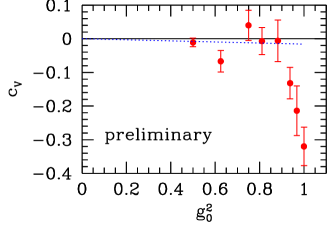
Figure 8: Non-perturbative improvement coefficient $c_{\rm V}$. One-loop bare perturbation theory is shown as a dotted line.

These correlation functions are related through the Ward identity ($t_{1}<x_{0}<t_{2}$)

$$Z_{\rm V} \left[k_{\rm V}(x_{0})+ac_{\rm V}\tilde{\partial}_{0}k_{\rm T}(x_{0})\right]$$

$$\,=Z_{\rm A}^{2}\left[k_{\rm AA}^{\rm I}(t_{2},x_{0})-k_{\rm AA}^{\rm I}(t_{1},x_{0})\right]+{\rm O}(a^{2}),$$

which is valid in the massless limit. Eq. (8) is derived in much the same way as the Ward identity discussed in the previous section. Inserting $Z_{\rm A},Z_{\rm V}$ and $c_{\rm A}$, it can be solved for the improvement coefficient $c_{\rm V}$.

The reader will by now be aware that, for a precise definition of the improvement condition, we have to make specific choices for $L,T,\theta,\ldots$. These, as well as a number of other details, will be given in ref. [33].

First results (cf. fig. 8) show $c_{\rm V}$ to be much larger than the perturbative estimate eq. (18) for couplings $g_{0}^{2}>0.9$. Its effect on vector meson decay constants and semileptonic decay form factors may be significant in simulations with presently achievable resolutions.

9 ${\rm O}(a^{2})$ EFFECTS

In sect. 2 we gave a perturbative example, where ${\rm O}(a)$ improvement removed most of the cutoff effects, leaving only tiny effects of higher order in the lattice spacing. Of course, it is important to check in how far this is true non-perturbatively.

9.1 The PCAC relation

The first test of ${\rm O}(a^{2})$ effects is provided again by the PCAC relation. To set the scale, remember that the cutoff effects in the PCAC mass $m$ were as large as several tens of ${\rm MeV}$ before improvement (cf. fig. 2). The situation after improvement, and for a somewhat larger value of the lattice spacing, is illustrated in fig. 9. Away from the boundaries, where the effect of states with energies of the order of the cutoff induces noticeable effects, $m$ is independent of time to within $\pm 2\,{\rm MeV}$.

Figure 9: Unrenormalized current quark mass $m$ in the improved theory, with non-perturbatively determined $c_{\rm sw}$ and $c_{\rm A}$, as a function of the time $x_{0}$ on a $32\times 16^{3}$ lattice at $\beta=6.2$ and $\kappa=0.1350$. The width of the corridor bounded by the dotted horizontal lines is $4\,{\rm MeV}$.

A search for other lattice artefacts after improvement yielded, as largest effect, the one described in the following.

Figure 10: Change $\delta\kappa_{\rm c}$ in the calculated value of $\kappa_{\rm c}$ when $L/a$ is increased from $8$ to $16$. The data have been obtained at $\beta=6.0,6.2$ and $6.4$ (from right to left). For $\beta>6.8$, $\delta\kappa_{\rm c}$ is consistent with zero within the statistical errors that are at most $10^{-5}$.

As chiral symmetry is violated by lattice artefacts, there is no precise definition of a chiral point $\kappa=\kappa_{\rm c}\equiv 1/(8+2am_{\rm c})$ for any finite value of the lattice spacing [9]. Rather, $\kappa_{\rm c}$ has an intrinsic uncertainty, which is reduced from ${\rm O}(a^{2})$ to ${\rm O}(a^{3})$ by non-perturbative improvement.

Here, we define $\kappa_{\rm c}$ as the value of $\kappa$, where $m$, eq. (30), vanishes for $C=C^{\prime}=\theta=0,T=2L,x_{0}=T/2$. To study the ${\rm O}(a^{3})$ effects we can then still vary the resolution $a/L$.

Close to $\kappa_{\rm c}$ the mass $m$ is a linear function of $\kappa$ to a high degree of accuracy. The point $\kappa_{\rm c}$ is therefore easily found by linear interpolation (or, for $\beta\leq 6.2$, slight extrapolation).

For $\beta>6.8$, the results for $a/L=1/8$ and $a/L=1/16$ agree on the level of their statistical accuracy, which is better than $10^{-5}$. For lower $\beta$, small but significant ${\rm O}(a^{3})$ effects are seen (fig. 10). They decrease rapidly as the lattice spacing is reduced.

9.2 Hadronic observables

It is of great interest to check the size of ${\rm O}(a^{2})$ terms in hadronic observables. At this conference first results for the improved theory have been presented by UKQCD [34] and we had the pleasure to survey the calculations of De Divitiis et al. [35] and Göckeler et al. [36]. Since all of these results are still preliminary, we restrict ourselves to some qualitative observations.

Wherever a comparison is possible, the results of the different groups are in good agreement. As the calculations were initiated only fairly recently, results to date exist for two values of the lattice spacing only, which correspond to $(a/r_{0})^{2}=0.035$ and $(a/r_{0})^{2}=0.019$. Although the lattice artefacts should therefore vary by roughly a factor of 2 between the two, a third, smaller value of $a$ appears necessary to perform precise extrapolations to the continuum limit.

Nevertheless, one observes [34, 36] that the lattice spacing dependence of the ratio of the vector meson mass to the square root of the string tension is reduced by improvement; indeed the values calculated in the improved theory are close to those computed without improvement and extrapolated to $a=0$. Unfortunately, it is not obvious that systematic errors in the determination of the string tension do not distort the picture. It would be desirable to repeat the analysis, replacing the string tension by $r_{0}$ [32].

The effect of the improvement of the axial current has been studied in the calculation of $f_{\pi}$. Despite the rather small value of the coefficient $c_{\rm A}$, the admixture of $\partial_{\mu}P$ represents a 10% change in $f_{\pi}$ at $(a/r_{0})^{2}=0.035$. After inclusion of this effect, $r_{0}f_{\pi}$ is independent of the lattice spacing within the statistical errors of around 3%.

In summary no large lattice artefacts have so far been found in the (quenched) improved theory. Improvement (and of course proper renormalization) of the composite fields is important in this respect.

10 DYNAMICAL FERMIONS

The ALPHA collaboration has started to implement improvement in full QCD with two flavours.

In particular, we are currently calculating $c_{\rm sw}(g_{0})$ along the lines described in section 6 [14]. We simulate with the Hybrid Monte Carlo algorithm [37] employing even-odd preconditioning of the Dirac operator and the Sexton–Weingarten scheme [38] for the integration of the equations of motion. The classical trajectories have unit length. For details of the implementation see ref. [39]. Alternative algorithms are being studied at the same time [40].

One slight difference from sect. 6 is that we do not insist on setting the improvement condition at $M=0$, but rather keep $aM$ small, say smaller than 0.02. Remember that the dependence of $\Delta M$ on $M$ is insignificant (cf. fig. 3). The reason for not attempting to put $M$ to zero exactly is not a difficulty in simulating in the massless limit. In the SF the massless Dirac operator has a gap [21], at least at not too large values of $L$, say $L\leq 1\,{\rm fm}$. Indeed, the simulations done so far show that it is irrelevant for the simulations whether we have $aM=0.02$ or $aM=0.001$. We do choose finite values of $M$ in order to avoid an unnecessarily large effort for tuning $M$.

Having said this, we mention, however, that as $g_{0}$ is increased at fixed $L/a=8$, the physical scale $L$ increases and the gap in the Dirac operator becomes smaller. This means that more Conjugate Gradient iterations are needed to obtain a solution of the Dirac equation. Quantitatively, in one hour on a 256-node APE-100, we obtain around 100 trajectories at $g_{0}^{2}=0.8$, 50 trajectories at $g_{0}^{2}=1$ and “only” 30 trajectories at $g_{0}^{2}=1.1$.

At the same time our autocorrelation times for typical long-range observables grow from roughly 1 trajectory at $g_{0}^{2}=0.5$ to 4 trajectories at $g_{0}^{2}=1.05$.

The simulations were started at small values of $g_{0}$ and reach $g_{0}^{2}=1.1$ by now.

In 1-loop perturbation theory [19], there is a shift in the bare coupling $\beta=6/g_{0}^{2}$ from the Wilson action to the improved action of $-0.3$ ($N_{\rm f}=2$). Using this and estimates of the lattice spacing with Wilson fermions [41], a rough estimate for the lattice spacing at $g_{0}^{2}=1.1$ is $0.1\,{\rm fm}$. We emphasize that this is a rough estimate since the true renormalization may be quite different at such a large value of the coupling. Nevertheless this indicates that $c_{\rm sw}$ will not be needed for values of $g_{0}^{2}$ that are much larger than $g_{0}^{2}=1.1$.

11 CONCLUSIONS

We have been able to implement on-shell O($a$) improvement non-perturbatively in (quenched) lattice QCD. The improvement coefficients $c_{\rm sw}$, $c_{\rm A}$, the critical mass $m_{\rm c}$ and the current normalization constants $Z_{\rm A}$ and $Z_{\rm V}$ have been determined for bare couplings in the range $0\leq g_{0}\leq 1$. In all cases, contact with bare perturbation theory could be made at couplings around $g_{0}^{2}\approx 0.25-0.5$. The convergence of perturbation theory appears to be significantly speeded up by tadpole improvement as shown by the crosses in figs. 5–7. However, for values of $\beta\leq 6.8$, which is the range most relevant for present MC computations, the quality of tadpole-improved perturbation theory is rather non-universal. There are examples such as $b_{\rm V},c_{\rm A}$, where perturbation theory is far off from our results. Renormalizations are large!

This suggests that one should be cautious when estimating improvement terms to a low order of perturbation theory, as is currently done in several attempts to extend improvement to the ${\rm O}(a^{2})$ level.

It is very pleasing that non-perturbative results can be obtained with statistical errors that are much smaller than the intrinsic ${\rm O}(\alpha^{2})$ uncertainties of the perturbative results for the improvement coefficients. The elimination of these perturbative uncertainties allows for reliable continuum extrapolations of the hadron spectrum and current matrix elements to be done in the future. Indeed, as a first step in this direction it was observed that residual ${\rm O}(a^{2})$ effects in hadronic quantities appear to be quite small. In particular, we point out that the $a$-independence of $r_{0}f_{\pi}$ was observed after accounting for the relatively large correction proportional to $c_{\rm A}$, a term that would have been set to zero in tree-level improvement and is still tiny at 1 loop.
Acknowledgements
I thank the organizers of this workshop for creating a very stimulating atmosphere and all the other members of the ALPHA collaboration for sharing their knowledge with me. I am grateful to M. Massetti and G. Schierholz for sending me results prior to publication. Most of the calculations discussed here have been obtained in the course of the ALPHA collaboration research programme. We thank DESY for allocating computer time on the APE-Quadrics computers to this project, and are grateful to the staff of the computer centre at DESY-IfH, Zeuthen for their support.

References

- [1] K. G. Wilson, Phys. Rev. D10 (1974) 2445
- [2] K. Jansen et al., Phys. Lett. B372 (1996) 275
- [3] See the example (fig. 1) given in R. Sommer, Nucl. Phys. B (Proc. Suppl.) 42 (1995) 186
- [4] K. Symanzik, in: Mathematical problems in theoretical physics, eds. R. Schrader et al., Lecture Notes in Physics, Vol. 153 (Springer, New York, 1982)
- [5] K. Symanzik, Nucl. Phys. B226 (1983) 187 and 205
- [6] M. Lüscher and P. Weisz, Commun. Math. Phys. 97 (1985) 59, E: Commun. Math. Phys. 98 (1985) 433
- [7] B. Sheikholeslami and R. Wohlert, Nucl. Phys. B259 (1985) 572
- [8] G.P. Lepage and P. Mackenzie, Phys. Rev. D48 (1993) 2250
- [9] M. Lüscher, S. Sint, R. Sommer and P. Weisz, Nucl. Phys. B478 (1996) 365
- [10] M. Lüscher and P. Weisz, Nucl. Phys. B479 (1996) 429
- [11] M. Lüscher, S. Sint, R. Sommer, P. Weisz and U. Wolff, Nucl. Phys. B491 (1997) 323
- [12] M. Lüscher, S. Sint, R. Sommer and H. Wittig, Nucl. Phys. B491 (1997) 344
- [13] S. Sint and P. Weisz, Further results on O(a) improved lattice QCD to one-loop order of perturbation theory, hep-lat/9704001
- [14] K. Jansen and R. Sommer, work in progress
- [15] F. Niedermeier, to be published in the proceedings of this workshop
- [16] P. Lepage, to be published in the proceedings of this workshop
- [17] M. Lüscher, R. Narayanan, P. Weisz and U. Wolff, Nucl. Phys. B384 (1992) 168
- [18] M. Lüscher, R. Sommer, P. Weisz and U. Wolff, Nucl. Phys. B389 (1993) 247, Nucl. Phys. B413 (1994) 481
- [19] S. Sint and R. Sommer, Nucl. Phys. B465 (1996) 71
- [20] R. Wohlert, Improved continuum limit lattice action for quarks, DESY 87-069 (1987), unpublished
- [21] S. Sint, Nucl. Phys. B421 (1994) 135, Nucl. Phys. B451 (1995) 416
- [22] G. Heatlie, G. Martinelli, C. Pittori, G. C. Rossi and C. T. Sachrajda, Nucl. Phys. B352 (1991) 266
- [23] K. Symanzik, Nucl. Phys. B190 [FS3] (1981) 1
- [24] M. Lüscher, Nucl. Phys. B254 (1985) 52
- [25] G. Parisi, in: High-Energy Physics — 1980, XX. Int. Conf., Madison (1980), ed. L. Durand and L. G. Pondrom (American Institute of Physics, New York, 1981)
- [26] M. Bochicchio, L. Maiani, G. Martinelli, G. Rossi and M. Testa, Nucl. Phys. B262 (1985) 331
- [27] L. Maiani and G. Martinelli, Phys. Lett. B178 (1986) 265
- [28] G. Martinelli, S. Petrarca, C.T. Sachrajda and A. Vladikas, Phys. Lett. B311 (1993) 241; E: B317 (1993) 660
- [29] E. Gabrielli, G. Martinelli, C. Pittori, G. Heatlie and C.T. Sachrajda, Nucl. Phys. B362 (1991) 475
- [30] M. Göckeler et al., Perturbative renormalization of bilinear quark and gluon operators, Talk given at the 14th International Symposium on Lattice Field Theory, St. Louis, 4-8 June 1996, Humboldt Univ. preprint HUB-EP-96/39, hep-lat/9608033
- [31] S. Sint, private notes (1996)
- [32] R. Sommer, Nucl. Phys. B411 (1994) 839
- [33] M. Guagnelli and R. Sommer, work in progress
- [34] R. Kenway, to be published in the proceedings of this workshop
- [35] G. M. de Divitiis, M. Massetti and R. Petronzio, work in progress
- [36] M. Göckeler, R. Horsley, H. Perlt, P. Rakow, G. Schierholz, A. Schiller and P. Stephenson, work in progress
- [37] S. Duane, A.D. Kennedy, B.J. Pendleton and D. Roweth, Phys. Lett. B195 (1987) 216
- [38] J. Sexton and D. Weingarten, Nucl. Phys. B380 (1992) 665
- [39] K. Jansen and C. Liu, Comput. Phys. Commun. 99 (1997) 221
- [40] R. Frezzotti and K. Jansen, DESY preprint DESY-97-020 (1996), hep-lat/9702016
- [41] U. Glässner et al. (SESAM Collaboration), Phys. Lett. B383 (1996) 98