The Schrödinger Functional for
Improved Gluon and Quark Actions
Timothy R. Klassen SCRI, Florida State University

Tallahassee, FL 32306-4052, USA

Abstract

The Schrödinger functional (quantum/lattice field theory with Dirichlet boundary conditions) is a powerful tool in the non-perturbative improvement and for the study of other aspects of lattice QCD. Here we adapt it to improved gluon and quark actions, on isotropic as well as anisotropic lattices. Specifically, we describe the structure of the boundary layers, obtain the exact form of the classically improved gauge action, and outline the modifications necessary on the quantum level. The projector structure of Wilson-type quark actions determines which field components can be specified at the boundaries. We derive the form of ${\rm O}(a)$ improved quark actions and describe how the coefficients can be tuned non-perturbatively. There is one coefficient to be tuned for an isotropic lattice, three in the anisotropic case.
Our ultimate aim is the construction of actions that allow accurate simulations of all aspects of QCD on coarse lattices.

1 Introduction

It has become generally recognized in the last few years that accurate continuum extrapolations of lattice QCD will be possible in the foreseeable future only by using improved actions (see e.g. [1]).

In the Symanzik (on-shell) improvement program [2, 3, 4, 5, 6], which we will follow, one systematically adds higher dimensional operators to an action, to cancel its lattice artifacts to some order in the lattice spacing $a$. Composite operators can be similarly improved. The coefficients of the improvement terms are trivial to calculate at tree-level; one-loop calculations are also possible, but already much more difficult, in general. Even if known, perturbative improvement coefficients per se are of limited value, since naive lattice perturbation theory does not work very well. It dramatically underestimates the improvement coefficients, for example.

Tadpole improved perturbation theory [7] works much better. For gluonic actions, where the leading errors of the Wilson plaquette action are ${\rm O}(a^{2})$, tree-level (or one-loop) plus tadpole improvement seems to cancel most of these errors, allowing quite accurate calculations on coarse lattices ($a=0.1-0.4$ fm, say), as several studies [8, 9, 10, 11] have demonstrated. Similarly, it seems that the leading ${\rm O}(a^{2})$ errors of the Wilson or Sheikholeslami-Wohlert (SW) [4] quark actions, which break rotational symmetry, can be cancelled to a large extent with classical and tadpole improvement. This is demonstrated by the excellent dispersion relations [12, 13] of the D234 [6] actions, for example.

On the other hand, for Wilson-type quark actions there are, at least at the quantum level, also ${\rm O}(a)$ violations of chiral symmetry. Even without the explicit non-perturbative determination of the ${\rm O}(a)$ improvement coefficient of the SW action (see below), there was clear evidence [15] that this coefficient is not estimated sufficiently accurately by tadpole improvement on coarse lattices. In any case, it is obviously preferable to determine at least the leading improvement coefficients non-perturbatively.

In seminal work, described in a series of papers (of which some are [16, 5, 14]), the ALPHA Collaboration has recently demonstrated how to do this. Using the Schrödinger functional [17, 18] and the demand that the PCAC relation hold for small quark masses, they determined the ${\rm O}(a)$ improvement coefficient of the SW quark action (as well as other quantities) on quenched Wilson glue. They find that it is almost 20% larger than the (plaquette) tree-level tadpole estimate even for a relatively fine $a\!=\!0.1$ fm lattice.

Motivated by these observations, our aim in this paper is to adapt the Schrödinger functional to improved gluon and quark actions.

The term “Schrödinger functional” is another name for the partition function of a euclidean quantum field theory with Dirichlet boundary conditions. In other words, one considers a theory with fixed boundary conditions on the fields at times $x_{0}=0$ and $x_{0}=T$, say. The Schrödinger functional is a powerful tool not just for the calculation of ${\rm O}(a)$ improvement coefficients of Wilson-type quark actions, but also for the determination of normalization and improvement coefficients of currents, as well as running couplings and quark masses. This is accomplished, in short, by using the finite volume and the boundary values of the gauge and quark fields as probes of the theory. Since Ward identities are local equations, they must hold independent of volume and boundary conditions. Probing the theory in this manner provides constraints that can be used to determine improvement coefficients. For the determination of running couplings one uses finite-size scaling techniques. One of the more technical reasons for the success of the Schrödinger functional is that the use of non-periodic boundary conditions in the time direction implies the absence of zero modes (at least for sufficiently small lattice spacings), allowing one to perform simulations directly at zero (or small) quark mass. This avoids a number of conceptual and practical complications.

For the case of pure gauge theory in the continuum it is quite clear what is meant (at least in a formal sense) by Dirichlet boundary conditions,

$${\cal Z}[C^{\prime},C]\,=\,\int\prod_{{\bf x}}\Lambda({\bf x})\int D[A]\,{\rm e}^{-S_{g}[A]}\,,\qquad S_{g}[A]\,=\,{1\over 4g^{2}}\int d^{4}x\,F_{\mu\nu}^{a}(x)F_{\mu\nu}^{a}(x)\,.$$ (1.1)

Here the path integral is over all gauge fields $A_{\mu}(x)$, $0\leq x_{0}\leq T$, with boundary values ($k=1,2,3$)

$$A_{k}(x)~{}=~{}\left\{\begin{array}[]{ll}C_{k}^{\Lambda}({\bf x})&\quad\mbox{at $x_{0}=0$}\\[2.84526pt] C^{\prime}_{k}({\bf x})&\quad\mbox{at $x_{0}=T$}\,,\end{array}\right.$$

where, generally, $C^{\Lambda}$ denotes the gauge field obtained after applying a gauge transformation $\Lambda$ to $C$.

For lattice QCD it is not immediately obvious how Dirichlet boundary conditions should be defined. The Schrödinger functional for pure gauge theory, in the form of the Wilson plaquette action, was studied in [18]; Wilson quarks were treated in [19]. For the case of improved gluon and quark actions considered here, we will see that the “boundary” in the Schrödinger functional will consist of a double layer of time slices. This causes slight complications at intermediate stages, but ultimately the Schrödinger functional formalism for improved actions proves to be hardly more complicated than for Wilson gluons and quarks.

There are several issues concerning the aims, scope and motivation of this paper that we should clarify at this point. First of all, the phrase “improved action” in the above is meant to refer to actions where at least the classical ${\rm O}(a^{2})$ errors have been eliminated by the addition of third and/or fourth order derivatives. Of course, in general it is inconsistent to consider improvement at order $a^{2}$ before having eliminated all errors at ${\rm O}(a)$. However, it is perfectly consistent to consider classical improvement to any order and then supplement it with quantum improvement to some lower order. It also makes sense to supplement classical with tadpole improvement.

For pure gauge theory perturbative improvement coefficients have been calculated to one loop for two actions [3, 20], so far. It is conceivable that at some point a practical method will be found to tune all gluonic $a^{2}$ errors to zero (at least for isotropic lattices). For fermions, on the other hand, this is clearly impossible; there are just too many terms at order $a^{2}$ [4]. This leads to an obvious question: If we can only eliminate ${\rm O}(a)$ but not all ${\rm O}(a^{2})$ errors, why should we even bother to eliminate what we hope are the leading $a^{2}$ errors via classical and tadpole improvement? We will argue that there are both theoretical and “empirical” reasons to suggest that this is a worthwhile enterprise. Let us discuss these reasons in turn. [The reader not interested in motivational issues, but only in the Schrödinger functional per se, can at this point skip ahead to the outline at the end of this section.]

Remember the special nature of the ${\rm O}(a)$ errors of Wilson-type quarks. They arise because we added a second-order derivative term to solve the doubler problem. This term breaks chiral symmetry, and, at least at the quantum level, ${\rm O}(a)$ errors become unavoidable. On the other hand, these terms do not break rotational symmetry at ${\rm O}(a)$ or ${\rm O}(a^{2})$. This is in contrast to the leading $a^{2}$ errors of both gluon and quark actions, which break rotational but not chiral symmetry. One might therefore argue that it is somewhat besides the point to label these errors as ${\rm O}(a)$ and ${\rm O}(a^{2})$ errors. Viewing them instead as the leading violations of chiral, respectively, rotational symmetry, it makes perfect sense to try to eliminate both of them as best as one can.

Now to the empirical reasons. Here the basic point is simply that the elimination of the leading ${\rm O}(a^{2})$ errors through classical and tadpole improvement works quite well. We already referred to the surprisingly accurate results obtained with improved gluon actions on coarse lattices. Concerning the more difficult case of ${\rm O}(a^{2})$ improved quark actions, I argued in [15], after surveying the available data, that all quantities with a weak dependence on the ${\rm O}(a)$ improvement term (dispersion relations, mass ratios) are also accurate to a couple percent on coarse lattices when calculated with such an action. It is only quantities with a relatively strong dependence on this term (like the $\rho$ mass in units of a gluonic scale such as the string tension, or the hyper-fine splitting of heavy quark systems) that still have significantly larger errors on the coarsest lattices. It is therefore not unreasonable to believe that with no ${\rm O}(a)$ and only small ${\rm O}(a^{2})$ errors accurate simulations of QCD will be possible on coarse lattices.

Concerning the gluon actions there is another more technical, but potentially important, issue we should mention. Namely, in addition to the ${\rm O}(a^{2})$ errors of the Wilson plaquette action, there also seem to be large non-power-like lattice artifacts that set in on lattices with spacings slightly above $0.1$ fm. What we are referring to is the non-trivial phase structure of the plaquette action when embedded in a larger space of couplings (fundamental and adjoint representations of the plaquette). This was the subject of many studies in the early days of lattice gauge theory; cf. [21] for recent results and references. The (in)famous dip of the discrete $\beta$-function, a similar dip in the $0^{++}$ glueball mass, and non-smooth behavior in various thermodynamic quantities are all believed to be consequences of a second-order phase transition close to the fundamental coupling axis of the Wilson gauge action. Although further studies are needed, there is evidence that these lattice artifacts are significantly smaller with improved gluon actions (see e.g. [11, 22]). There are also more direct indications that the second-order phase transition point moves away from the fundamental coupling axis with improvement [23]. Finally, it seems that the variance of the static potential measured with improved glue [8, 24] is much smaller than for Wilson glue at the same lattice spacing. This might also be related to the phase structure (on the other hand, there might be more prosaic reasons for this; this remains to be investigated).

The potential significance of these issues is as follows. In their study of the ${\rm O}(a)$ improvement of the SW action on quenched Wilson glue Lüscher et al found [14] that the improvement coefficient could not be determined for lattices coarser than $0.1$ fm, due to large fluctuations (“exceptional configurations”) of the glue, leading to accidental zero modes at small quark mass. In the quenched approximation this problem is bound to occur at some sufficiently coarse lattice spacing, but it is not clear a priori exactly where it should occur. It could depend on the specific lattice action used. The observations described in the previous paragraph, lead one to hope that with improved glue the breakdown will occur on coarser lattices.

While finishing the write-up of this paper, hard facts began to emerge that support the above arguments: As will be described in [25], the breakdown of the quenched approximation does indeed occur on coarser lattices when improved glue is used.

The hope that this would happen was the main motivation underlying this paper. To obtain accurate continuum results from lattice QCD requires simulations at a series of lattice spacings that provide a significant “lever arm” for extrapolations. Due to the dramatic increase in the cost of a QCD simulation as the lattice spacing is decreased, such a series can be obtained orders of magnitude cheaper if one makes use of coarse lattices.

Concerning the scope of this paper we should mention that we will also consider anisotropic lattices [6, 26, 27]. Such lattices, with a smaller temporal than spatial lattice spacing, offer the best hope to tackle certain hard problems, like the simulation of heavy quarks in a relativistic formalism [13, 6] and detailed studies of glueballs [22]. Due to the breaking of manifest space-time exchange symmetry on anisotropic lattices, there are more terms that have to be tuned to eliminate all ${\rm O}(a)$ errors of a Wilson-type quark action (as we will discuss). Tuning these errors to zero is therefore more complicated, but should be within reach of the Schrödinger functional technology (cf. sect. 4). Note that anisotropic lattices fit quite naturally into the Schrödinger functional framework, since the boundary conditions already treat space and time differently.

The outline of this paper is as follows. In sect. 2 we derive the Schrödinger functional for improved gluon actions. We discuss the structure of the boundary layers and the precise form of the (classical) action at the boundaries, where the fields are given fixed values. We then specialize to spatially constant boundary values and discuss the classical background field they induce in the bulk, including its uniqueness. The subject of sect. 3 is Dirichlet boundary conditions for (improved) quark actions. All Wilson-type quark actions of practical interest, on isotropic as well as anisotropic lattices, have a certain projector structure, which dictates which field components can be fixed at the boundaries. Once these are specified, one can define boundary quark fields as functional derivatives with respect to the boundary values. These boundary fields are extremely useful in applications of the Schrödinger functional. One application is described in sect. 4, namely, the determination of the ${\rm O}(a)$ improvement coefficients of Wilson-type quark actions. Concluding remarks and a brief discussion of future work can be found in sect. 5.

Appendix A summarizes some of our notation and conventions. In appendix B we discuss the classical boundary errors of the pure gauge Schrödinger functional. In appendix C, finally, we derive the form of ${\rm O}(a)$ on-shell improved quark actions on anisotropic lattices. We also recall [4, 6] the classical improvement of quark actions.

This paper is largely self-contained, but the reader might want to consult [18] for a detailed introduction to the Schrödinger functional, ref. [16] for a summary of various applications, and [5, 6] for discussions of Symanzik improvement for fermions.

2 Gauge Fields

2.1 Gauge Actions in the Bulk

Consider a four-dimensional hypercubic lattice of extent $L_{\mu}$ and lattice spacing $a_{\mu}$ in direction $\mu=0,1,2,3$. Except for purely classical considerations we assume the lattice to be spatially isotropic with $a\equiv a_{k},\,k\!=\!1,2,3$. Other notations and conventions are summarized in appendix A.

To avoid having to worry about boundary effects at this point, let us impose periodic boundary conditions on the gauge fields for the moment. The lattice gauge actions of interest can be written as

$$S_{g}[U]\,=\,{2\over g^{2}}\sum_{\tau}\sum_{{\cal C}\in{\cal S}_{\tau}}c_{\tau}\,{\rm Re}\,\hbox{Tr}\,[1\,-\,U({\cal C})]\,,$$ (2.2)

where $U({\cal C})$ denotes the product of link fields along the loop ${\cal C}$, $\tau$ labels a finite set of types of loops, and ${\cal S}_{\tau}$ is the set of all positively oriented (say) loops of a given type that can be drawn on the lattice. On an isotropic lattice the types of loops might include plaquettes, rectangles, etc; on an anisotropic lattice one would have to distinguish spatial plaquettes, temporal plaquettes, spatial rectangles, short-temporal rectangles, long-temporal rectangles, etc.

The real numbers $c_{\tau}$ are determined by some improvement condition. We do not really need to know the exact numbers to set up the Schrödinger functional, but for concreteness let us be more explicit about a simple class of actions that is sufficient to illustrate what happens for more general improved actions. Namely, for “plaquette $+$ rectangle” actions [28] we can write

$$S_{g}[U]\,=\,{2\over g^{2}}\,\sum_{x,\,\mu<\nu}{\Delta V\over a_{\mu}^{2}a_{\nu}^{2}}\,{\rm Re}\,\hbox{Tr}\,\left[c^{(0)}_{{\mu\nu}}\,\frac{1-P_{{\mu\nu}}(x)}{u_{\mu}^{2}u_{\nu}^{2}}\,-\,c^{(1)}_{\mu}\,\frac{1-R_{{\mu\nu}}(x)}{u_{\mu}^{4}u_{\nu}^{2}}\,-\,c^{(1)}_{\nu}\,\frac{1-R_{\nu\mu}(x)}{u_{\nu}^{4}u_{\mu}^{2}}\right]\,,$$ (2.3)

where $\Delta V=\prod_{\mu}a_{\mu}$ is the volume of a single lattice hypercube, and $P_{\mu\nu}$ and $R_{\mu\nu}$ are equal to $U({\cal C})$ with ${\cal C}$ a $1\times 1$ (plaquette), respectively, $2\times 1$ (rectangle) Wilson loop in the ${\mu\nu}$ plane. The coefficients $c^{(0)}_{{\mu\nu}}=1+4(c^{(1)}_{\mu}+c^{(1)}_{\nu})$ and for good measure we have also indicated tadpole improvement factors $u_{\mu}$ that one might want to include. As special cases this class of actions contains the Wilson and tree-level ${\rm O}(a^{2})$ improved [28, 3] actions,

$$c^{(1)}_{\mu}~{}=~{}\left\{\begin{array}[]{cl}0&\quad\mbox{Wilson action}\\[2.84526pt] {1\over 12}&\quad\mbox{Improved action}\,.\end{array}\right.$$

Another interesting case, on anisotropic lattices, is defined by $c^{(1)}_{\mu}={1\over 12}(1-\delta_{\mu 0})$ (cf. [27]). Only the spatial directions are improved now; there are no tall-temporal rectangles in the action, leading to $a_{0}^{2}$ errors. Since this action contains only loops of maximal temporal extent $1$, there are no unphysical branches in its dispersion relation.

2.2 Transfer Matrix

The Schrödinger functional can either be defined as the partition function with fixed boundary conditions, or as a suitable power of the transfer matrix evaluated between initial and final states. On the lattice the meaning of “fixed boundary conditions” is not a priori clear. Understanding this issue via the transfer matrix is at least pedagogically useful, so we will proceed by reviewing the transfer matrix formalism. For improved gauge actions this formalism was described in [29], whose approach we will follow.

We will use the plaquette $+$ rectangle actions as examples, but as we proceed it will become clear how to construct the transfer matrix for more general actions. We will also see that the general form of the transfer matrix is determined solely by the maximal temporal extent of the loops appearing in the action. To avoid tedious and irrelevant case distinctions, we will use the term “Wilson action” as a shorthand for any gauge action with loops of maximal temporal extent $1$. Note that this also includes plaquette $+$ rectangle actions without tall-temporal rectangles, which, as mentioned earlier, are useful for anisotropic lattices. We will use the phrase “improved action” to denote actions with loops of maximal temporal extent $2$.

For pedagogic reasons we first consider the Wilson case. The classical lattice field equations for such actions (in temporal gauge $U_{0}(x)\equiv 1$, say) are second order difference equations in $x_{0}$. Specifying the link field on one initial and one final time slice leads to a unique solution to the field equations. The transfer matrix of the quantum theory should therefore give the amplitude to go from some gauge field on one time slice to another field on some other time slice.

To define the transfer matrix we first have to specify the Hilbert space ${\cal H}$ on which it is supposed to act. We take ${\cal H}$ to consist of wave functions $\varphi[U]$ that are functions of the gauge field $U$ on a fixed time slice, with the natural inner product

$$\langle\varphi_{2}|\varphi_{1}\rangle\,=\,\int D[U]~{}\varphi_{2}[U]^{\ast}\,\varphi_{1}[U]~{},\qquad\quad D[U]\,\equiv\,\prod_{{\bf x},k}\,dU_{k}({\bf x})~{},$$ (2.4)

in terms of the Haar measure $dU$ on SU($N$). More precisely, ${\cal H}$ consists of all gauge invariant wave functions of finite norm. Note that any wave function can be made gauge invariant by averaging over gauge transformations $U\rightarrow U^{\Lambda}$. This defines a projection operator onto the physical subspace,

$$\mathchoice{\sf I\kern-1.4pt{P}}{\sf I\kern-1.4pt{P}}{\sf I\kern-1.1pt{P}}{\sf I\kern-1.1pt{P}}\varphi[U]\,=\,\int\prod_{{\bf x}}\,d\Lambda({\bf x})\,\varphi[U^{\Lambda}]\,.$$ (2.5)

We can write $\varphi[U]=\langle U|\varphi\rangle$ where the states $|U\rangle$ are eigenstates of the link field operators $\hat{U}_{k}(x)$ in the Schrödinger representation, with eigenvalues $U_{k}(x)$. For gauge invariance the projector $\mathchoice{\sf I\kern-1.4pt{P}}{\sf I\kern-1.4pt{P}}{\sf I\kern-1.1pt{P}}{\sf I\kern-1.1pt{P}}$ should be applied to the $|U\rangle$’s, which will be understood in the following. The identity can be decomposed as $1\kern-2.5pt{\rm l}=\int D[U]\,|U\rangle\langle U|$.

The transfer matrix $\mathchoice{\sf T\kern-5.20004pt{T}}{\sf T\kern-5.20004pt{T}}{\sf T\kern-3.99994pt{T}}{\sf T\kern-3.99994pt{T}}$ acts on wave functions as

$$(\mathchoice{\sf T\kern-5.20004pt{T}}{\sf T\kern-5.20004pt{T}}{\sf T\kern-3.99994pt{T}}{\sf T\kern-3.99994pt{T}}\varphi)[U^{\prime}]\,=\,\int D[U]~{}\langle U^{\prime}|\mathchoice{\sf T\kern-5.20004pt{T}}{\sf T\kern-5.20004pt{T}}{\sf T\kern-3.99994pt{T}}{\sf T\kern-3.99994pt{T}}|U\rangle\,\varphi[U]~{},$$ (2.6)

where its matrix element (or kernel) to go from gauge field $U$ at time $t$ to $U^{\prime}$ at time $t+a_{0}$ is given by

$$\langle U^{\prime}|\mathchoice{\sf T\kern-5.20004pt{T}}{\sf T\kern-5.20004pt{T}}{\sf T\kern-3.99994pt{T}}{\sf T\kern-3.99994pt{T}}|U\rangle\,=\,\int\prod_{{\bf x}}dV_{0}(t,{\bf x})~{}{\rm e}^{-\Delta S[U^{\prime},V_{0},U]}~{},\qquad\quad V_{0}(t,{\bf x})\in{\rm SU}(N)~{}.$$ (2.7)

Here $\Delta S[U^{\prime},V_{0},U]$ is given by exactly the same expression as the action itself, restricted to a two time slice lattice with gauge fields $U$ at $t$, $U^{\prime}$ at $t+a_{0}$, and $V_{0}$ playing the role of the temporal link fields — except that the contribution from loops completely within the spatial planes at $t$ and $t+a_{0}$ are weighted with a factor of ${\textstyle{1\over 2}}$. This is illustrated in figure 1. It is clear why this factor of ${\textstyle{1\over 2}}$ must be present: When we take powers of the transfer matrix (to get the partition function or Schrödinger functional, see below) all gauge fields on the internal time slices contribute twice. Similarly, a correlation function involving gauge fields is equal to some power of the transfer matrix with operators $\hat{U}$ inserted at appropriate places in the product.

   

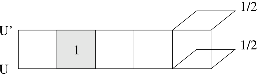
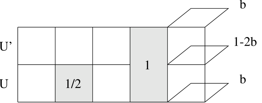
Figure 1: Temporal weight factors of various loops for Wilson (left) and improved (right) action transfer matrices.

We now turn to the ${\rm O}(a^{2})$ improved case. With loops in the action extending up to two steps in the temporal direction, the action involves second order, the field equations fourth order temporal differences (in temporal gauge). There will be a unique solution to the field equations if we specify the gauge field on two initial and two final time slices. Correspondingly, we expect the Hilbert space to consist of wave functions on two consecutive time slices, and the transfer matrix to give the amplitude for transitions between such double layers.

Let

$$\varphi[U]~{}\equiv~{}\varphi[U^{(+)},U^{(0)},U^{(-)}]$$ (2.8)

be a wave function depending on the link field $U^{(-)}$ on time slice $t$, $U^{(+)}$ on time slice $t+a_{0}$, as well as the temporal links $U^{(0)}$ connecting the two time slices. Let the Hilbert space consist of gauge invariant wave functions of finite norm, with respect to the inner product

$$\langle\varphi_{2}|\varphi_{1}\rangle\,=\,\int D[U]~{}\varphi_{2}[U]^{\ast}\,\varphi_{1}[U]~{},\qquad D[U]\,\equiv\,\prod_{{\bf x}}\Bigl{[}dU^{(0)}({\bf x})\prod_{k}\,dU^{(+)}_{k}({\bf x})\,dU^{(-)}_{k}({\bf x})\Bigr{]}\,.$$ (2.9)

The transfer matrix is then defined by

$$\langle U^{\prime}|\mathchoice{\sf T\kern-5.20004pt{T}}{\sf T\kern-5.20004pt{T}}{\sf T\kern-3.99994pt{T}}{\sf T\kern-3.99994pt{T}}|U\rangle\,=\,{\rm e}^{-\Delta S[U^{\prime},U]}~{}\prod_{{\bf x},k}~{}\delta\Bigl{(}U^{\prime(-)}_{k}({\bf x}),\,U^{(+)}_{k}({\bf x})\Bigr{)}~{}.$$ (2.10)

The $\delta$-function (with respect to the Haar measure) means that the transfer matrix is effectively a “$2\rightarrow 1$” and not a “$2\rightarrow 2$” time slice operator. $\Delta S[U^{\prime},U]$ is the action of a three time slice lattice obtained by fusing the top layer $U^{(+)}$ of $U$ with the bottom layer $U^{\prime(-)}$ of $U^{\prime}$, where we weigh a Wilson loop of temporal extent $\Delta t$ (in lattice units) by a factor

$$w(\Delta t\!=\!2)=1\,,\quad w(\Delta t\!=\!1)={1\over 2}\,,\quad w(\Delta t\!=\!0)=\left\{\begin{array}[]{cl}b&\quad\mbox{at $x_{0}=t$}\\ 1-2b&\quad\mbox{at $x_{0}=t+a_{0}$}\\ b&\quad\mbox{at $x_{0}=t+2a_{0}$}\end{array}\right.$$

This is presented graphically in figure 1. Note that $\langle U^{\prime}|\mathchoice{\sf T\kern-5.20004pt{T}}{\sf T\kern-5.20004pt{T}}{\sf T\kern-3.99994pt{T}}{\sf T\kern-3.99994pt{T}}|U\rangle$ is gauge invariant, since $\Delta S$ is.

Time reflection symmetry dictates the above form of the “temporal weight factors” $w(\Delta t)$. When taking powers of the transfer matrix the $w(\Delta t)$ combine to give $1$ for all loops in the bulk, ensuring that we obtain the correct (bulk) partition and correlation functions. This is true for any value of the (real) parameter $b$. The effect of $b$ is only noticeable at the boundaries. Its value is fixed, classically, by demanding the absence of order $a^{2}$ boundary errors. This will be discussed in the next subsection and appendix B. Let us for the moment keep $b$ a free parameter.

The transfer matrix of improved actions is not hermitean [29], since energy eigenvalues are complex at the order of the cutoff (this can also be seen by studying the dispersion relation). In most situations the resulting effects, chiefly oscillatory behavior of correlation functions at small times, do not create significant problems in practice.

2.3 Gauge Actions with Dirichlet Boundary Conditions

We can now write down gauge actions with Dirichlet boundary conditions. We choose the spatial boundary conditions on the gauge fields to be periodic. To obtain the Schrödinger functional on a lattice of temporal extent $T/a_{0}$ we just have to evaluate $\mathchoice{\sf T\kern-5.20004pt{T}}{\sf T\kern-5.20004pt{T}}{\sf T\kern-3.99994pt{T}}{\sf T\kern-3.99994pt{T}}^{T/a_{0}}$ between fixed initial and final states. In the Wilson case the gauge fields have to be specified at $x_{0}=0$ and $x_{0}=T$, in the improved case on the $x_{0}=-a_{0},0$ and $x_{0}=T^{\prime},T^{\prime}+a_{0}$ double layers. To allow for a unified notation for the Wilson and improved cases in various formulas, we have introduced

$$T^{\prime}~{}\equiv~{}\left\{\begin{array}[]{ll}T&\quad\mbox{Wilson action}\\[2.84526pt] T\,-\,a_{0}&\quad\mbox{Improved action}~{}.\end{array}\right.$$

Denoting the boundary gauge fields by $W$ and $W^{\prime}$, we define the Schrödinger functional for pure gauge theory as

$${\cal Z}[W^{\prime},W]\,=\,\langle W^{\prime}|\mathchoice{\sf T\kern-5.20004pt{T}}{\sf T\kern-5.20004pt{T}}{\sf T\kern-3.99994pt{T}}{\sf T\kern-3.99994pt{T}}^{T/a_{0}}|W\rangle\,.$$ (2.11)

Remember that in the improved case $W$ is a shorthand for the fields $W^{(+)},W^{(0)},W^{(-)}$ on a double layer (and ditto for $W^{\prime}$). More explicitly, we can write

$${\cal Z}[W^{\prime},W] \!=\! \int D[U]\,e^{-S_{g}[U;W^{\prime},W]}\,\,,\qquad D[U]\,\equiv\,\prod_{{\bf x}}\,\Biggl{[}dU_{0}(0,{\bf x})\,\prod_{x_{0}=a_{0}}^{T^{\prime}-a_{0}}\,\prod_{\mu}\,dU_{\mu}(x)\Biggr{]}$$

$$S_{g}[U;W^{\prime},W] \!=\! {2\over g^{2}}\sum_{\tau}\sum_{{\cal C}\in{\cal S}_{\tau}}\,w({\cal C})\,c_{\tau}\,{\rm Re}\,\hbox{Tr}\,[1\,-\,U({\cal C})]\,,$$ (2.12)

where the temporal weight factor $w({\cal C})$ for a loop in an action with Dirichlet boundary conditions is best defined pictorially, as in figure 2.

   

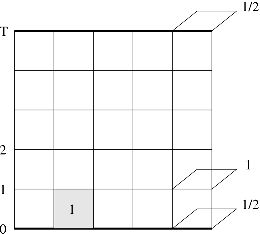
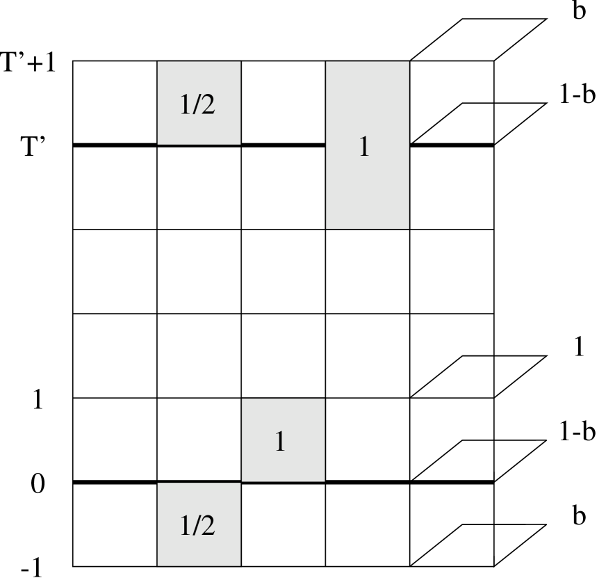
Figure 2: Temporal weight factors of various loops in the Wilson (left) and improved (right) actions with Dirichlet boundary conditions on lattices with $L=5a$ and $T=5a_{0}$. Time, measured in lattice units, runs upwards, as marked on the left ($T^{\prime}\equiv T-1$ for the improved case). The thick lines indicate the boundaries of the bulk region; every loop with at least one link strictly inside the bulk has a temporal weight factor of $1$.

As remarked in the caption of this figure, all loops containing a dynamical link have a temporal weight factor of $1$. This fact simplifies the coding of the updating algorithm for the Schrödinger functional.

We now discuss the boundary errors of the Schrödinger functional. In particular we have to fix the so far free parameter $b$ in the improved case. In view of the remark in the previous paragraph, the reader might wonder at this point, how errors associated with the boundary fields, which are, after all, fixed in a simulation, can have any effect on an observable defined in terms of dynamical variables in the bulk.

First of all, even on the classical level it is legitimate to consider observables defined by taking functional derivatives with respect to the boundary values, and only then fixing them at some suitable value. This introduces cross terms between the bulk and the boundary fields. The “SF coupling” defined in [30], for example, does involve such derivatives. Secondly, on the quantum level the boundary effects can “spill into the bulk” and affect the dynamics there, as we will see shortly.

Let us first consider the classical boundary errors of the Schrödinger functional. We want to know the difference between the lattice and the continuum actions with corresponding boundary conditions. This difference has two sources. One is the difference between the continuum and lattice action densities (the integrand/summand), the other the difference between an integral and a discrete sum approximating it.

This is basically a classical calculus problem; the elementary, if slightly wordy, tracking of the differences for the Wilson and improved actions is discussed in appendix B. We here only state the conclusion: The Wilson action has order $a^{2}$ boundary errors, and the improved action only $a^{4}$ errors if we choose $b=1/24$.

Actually, at tree level the precise value of $b$ does not matter for the special (spatially constant) boundary values of the gauge field we will consider later. For many applications this is even true on the quantum level at ${\rm O}(a)$; a point to which we will return in a moment.

In the quantum case it is expected [17, 18] that in addition to the usual counter terms in the bulk, some small number of additional counter terms might be necessary on the boundaries. In pure gauge theory the only possible terms at ${\rm O}(a)$ are spatial sums over the boundary time slices of lattice versions of $\hbox{Tr}\,F_{0k}^{2}$ and $\hbox{Tr}\,F_{kl}^{2}$. Note that there is no difference in this respect between isotropic and anisotropic lattices (in contrast to the bulk, where fewer counter terms are necessary in the isotropic case).

So, no terms not already present in the classical action are required on the quantum level. In addition to the usual renormalization of the gauge coupling in the bulk (and other bulk renormalizations for anisotropic lattices; see [27], and for first one-loop results [31]), there will be corrections to the weight factors of some of the loops at the boundary. It is interesting to note that to obtain the counter term for $\hbox{Tr}\,F_{0k}^{2}$ in the Wilson case by necessity affects the temporal weight factor of plaquettes involving dynamical links (namely the temporal plaquettes touching the boundaries at $x_{0}\!=\!0$ and $x_{0}\!=\!T$), whereas for the improved case one can choose to renormalize only the weight factors of temporal plaquettes within the boundary doubler layers, which do not involve dynamical links. To obtain the counter term for $\hbox{Tr}\,F_{kl}^{2}$ one can, in both cases, suitably adjust the weight factor of spatial plaquettes within the boundary.

This means that for the improved case some observables will not be sensitive to ${\rm O}(a)$ quantum errors incurred by the wrong choice of the temporal and spatial plaquette coefficients in the boundary; only observables involving derivatives with respect to the boundary values that lead to a coupling of the dynamical links with the boundary plaquettes will “see” such errors.

In any case, though, for most applications of the Schrödinger functional it is not important to know the boundary counter terms. The basic reason has already been mentioned in the introduction: The boundary fields are used to probe the local dynamics of the theory, which, to leading order, should be independent of the precise details of the boundary terms, including their renormalization (see [5] for a formal proof).

2.4 The Classical Background Field

The boundary values of the gauge field induce some classical background field in the bulk. It is important, e.g. for perturbative calculations, that the background field be unique (up to gauge equivalence). This will not be the case for an arbitrary choice of boundary values. Spatially constant boundary values have turned out to be both convenient and sufficient for all applications of the Schrödinger functional (so far, at least). Physically, these boundary conditions correspond to a constant color-electric background field. We will first consider generic boundary conditions of this type and later discuss further restrictions that have to be imposed when we turn to the question of uniqueness.

In the continuum the background gauge field in such a situation, denoted by $\bar{A}_{\mu}(x)$, is given by

$$\bar{A}_{0}(x)\,=\,0~{},\qquad\bar{A}_{k}(x)\,=\,{1\over T}\left[x_{0}C^{\prime}_{k}+(T-x_{0})C_{k}\right]~{}.$$ (2.13)

Here $C_{k}$ and $C^{\prime}_{k}$ are the (hermitean) boundary values of the gauge field,

$$\bar{A}_{k}(x)~{}=~{}\left\{\begin{array}[]{ll}C_{k}&\quad\mbox{at $x_{0}=0$}\\[2.84526pt] C^{\prime}_{k}&\quad\mbox{at $x_{0}=T$}~{},\end{array}\right.$$

in terms of which the color-electric field strength reads $\bar{F}_{0k}=(C^{\prime}_{k}-C_{k})/T$.

If one assume that $C_{k}$ and $C^{\prime}_{k}$ commute (e.g. if they are diagonal, see below), then an obvious guess for the background field on the lattice is $\bar{U}_{\mu}(x)=\exp(-ia_{\mu}\bar{A}_{\mu}(x))$, or explicitly,

$$\bar{U}_{0}(x)\,=\,1~{},\qquad\bar{U}_{k}(x)\,=\,\exp\Bigl{(}-i{a_{k}\over T}[x_{0}C^{\prime}_{k}+(T-x_{0})C_{k}]\Bigr{)}~{}.$$ (2.14)

For the Wilson case this corresponds to the boundary values

$$\bar{U}_{k}(x)~{}=~{}\left\{\begin{array}[]{ll}W_{k}({\bf x})\,=\,e^{-ia_{k}C_{k}}&\qquad\mbox{at $x_{0}=0$}\\[2.84526pt] W^{\prime}_{k}({\bf x})\,=\,e^{-ia_{k}C^{\prime}_{k}}&\qquad\mbox{at $x_{0}=T$}~{}.\end{array}\right.$$

For improved actions one can read off the boundary fields $W_{k}^{(\pm)}$ and $W^{\prime(\pm)}_{k}$ from (2.14) at $t=-a_{0},0$ and $t=T^{\prime},T^{\prime}+a_{0}$, respectively. $W^{(0)}({\bf x})=1=W^{\prime(0)}({\bf x})$, of course.

It remains to be proved that (2.14) actually is the correct background field on the lattice. To this end, note that for this field the non-vanishing contributions to the action come from the temporal plaquette and rectangle terms,

$$P_{0k}(x)\,=\,P_{k0}(x)^{\ast} = \exp\Bigl{(}-i{a_{0}a_{k}\over T}[C^{\prime}_{k}-C_{k}]\Bigr{)}~{},$$

$$R_{0k}(x)\,=\,R_{k0}(x)^{\ast} = \exp\Bigl{(}-2i{a_{0}a_{k}\over T}[C^{\prime}_{k}-C_{k}]\Bigr{)}~{}.$$ (2.15)

The contribution of a loop to an arbitrary gauge action is simply related to the color-electric flux through the loop. Since the background electric field is constant in space and time, the same is true for these fluxes, which implies that (2.14) obeys the lattice field equations for any gauge action. The uniqueness of the background field (2.14) will be discussed in the next subsection.

The fact that (2.14) satisfies the field equations for an arbitrary gauge action, testifies to the “quality” of the abelian boundary fields, as previously remarked in [18]. This can also be seen by calculating the value of the plaquette $+$ rectangle action (2.3) for the background field with Schrödinger functional boundary conditions,

$$S_{g}[\bar{U}] \!=\! {TL_{1}L_{2}L_{3}\over g^{2}}\,\sum_{k}\,\hbox{Tr}\,\Bigl{(}{2\over a_{0}a_{k}}\sin\alpha_{k}\Bigr{)}^{2}\,\Bigl{(}1+4(c^{(1)}_{k}+c^{(1)}_{0})\sin^{2}\alpha_{k}\Bigr{)}$$ (2.16)

$$\!=\! {L_{1}L_{2}L_{3}\over g^{2}T}\,\sum_{k}\hbox{Tr}\,(C^{\prime}_{k}-C_{k})^{2}\,+\,{\rm O}(a^{4})\>,\quad\alpha_{k}\equiv{a_{0}a_{k}\over 2T}(C^{\prime}_{k}-C_{k})~{}.$$

The same result would have been obtained with periodic boundary conditions in the time direction. We see that for constant abelian boundary fields even the Wilson action has only ${\rm O}(a^{4})$ errors relative to the continuum limit.

2.5 Uniqueness of the Classical Background Field

It is important to know if, for given boundary values of the gauge field, the background field is the unique (up to gauge equivalence) absolute minimum of the action.

In ref. [18] a theorem establishing uniqueness was provided for the Wilson plaquette action, in any number of dimensions, for a certain class of diagonal and spatially constant boundary values. To specify this class consider diagonal boundary values

$$C_{k}\,=\,{1\over L_{k}}\pmatrix{\phi_{k1}&0&\ldots&0\cr 0&\phi_{k2}&\ldots&0\cr\vdots&\vdots&\ddots&\vdots\cr 0&0&\ldots&\phi_{kN}\cr}$$ (2.17)

and similarly for $C^{\prime}_{k}$ in terms of a set of $\phi^{\prime}_{k\alpha}$. Gauge symmetry implies that the $\phi_{k\alpha}$ and $\phi^{\prime}_{k\alpha}$ have angular character; we can always choose them to lie in $(-\pi,\pi]$. A vector $(\phi_{1},\ldots,\phi_{N})$ is said to lie in the fundamental domain if

$$\sum_{\alpha}\,\phi_{\alpha}=0\,,\quad\phi_{1}<\phi_{2}<\ldots<\phi_{N}\,,\quad\phi_{N}-\phi_{1}<2\pi\,.$$ (2.18)

It was proved in [18] that a sufficient condition for the uniqueness of the background field (2.14) is that the vectors $\phi_{k}$, $\phi^{\prime}_{k}$ (defined in the obvious way) lie in the fundamental domain. The theorem also holds if some or all of the $\phi_{k}$ or $\phi^{\prime}_{k}$ are zero (vectors).

The proof given in [18] for the Wilson action is quite involved. As a corollary it implies that the analogous theorem holds in the continuum. One therefore expects such a theorem to hold for improved actions, since they are supposedly more continuum-like than the Wilson action. However, there is at least one step in the proof, related to the use of the field equations, that prevents a straightforward extension to improved actions.

Even though uniqueness presumably holds for all “reasonable” improved actions, we have no proof at the moment. We have therefore investigated the question of uniqueness numerically. For various actions, volumes and boundary conditions we started with some random initial configurations, and used simulated annealing to find a minimum of the action. Besides the plaquette $+$ rectangle action, we considered the action with an additional “parallelogram” term, i.e. a set if loops sufficient for full order $a^{2}$ improvement [3]. We stepped through the region of improvement coefficients of interest in practice — and beyond. Several boundary values in (and on the boundary of) the fundamental domain were considered. In all cases where the coefficients of the improvement terms are such that positivity holds (cf. [3]; any viable action must satisfy positivity), the simulated annealing algorithm eventually converged to the classical background field (2.14).

We should add that we found the above to be true even on the very small lattices, like $L\!=\!2a$, $T\!=\!3a$, where the proof of [18] does not apply. The only cases we could find where the global minimum is definitely not given by (2.14) involve actions with large negative coefficients for the improvement terms, violating positivity. Then indeed rather interesting things can happen. The simplest, and surprisingly rich, example is provided by the plaquette $+$ rectangle action on a two-dimensional lattice with $L\!=\!2a$, $T\!=\!3a$ and vanishing boundary fields, $\phi=0=\phi^{\prime}$. For a certain region of large negative rectangle coefficient, for instance, there is a discrete set of degenerate vacua that break spatial translation symmetry. The vacua have an anti-ferromagnetic character, in that translation invariance holds only under shifts by two lattice units.

We conclude that for boundary values in the fundamental domain all improved actions of interest in practice seem to have the expected unique global minimum for arbitrary volumes.

3 Fermions

3.1 Fermion Actions in the Bulk

Before writing down the most general quark action

$$S_{q}[{\bar{\psi}},\psi,U]~{}=~{}a_{0}a^{3}\,\sum_{x}\,{\bar{\psi}}(x)\,Q\,\psi(x)$$ (3.19)

we will be interested in, let us consider two important special cases on isotropic lattices. These are the “isotropic SW” [4] and the “isotropic D234” [6] actions, whose quark matrices $Q$ can be written as

$$Q_{W_{1}} \!=\! m_{0}\,-\,a\,{\omega\over 4}\,\sigma\!\cdot\!F\,+\,\sum_{\mu}\gamma_{\mu}W_{\mu}~{},$$

$$Q_{W_{2}} \!=\! m_{0}\,-\,a\,{\omega\over 6}\,\sigma\!\cdot\!F\,+\,\sum_{\mu}\,\Bigl{(}\gamma_{\mu}W_{\mu}+{a\over 6}W_{\mu}^{2}\Bigr{)}~{},$$ (3.20)

in terms of the “Wilson operator”

$$W_{\mu}~{}\equiv~{}\nabla_{\mu}-{a_{\mu}\over 2}\gamma_{\mu}\Delta_{\mu}\>.$$ (3.21)

We will therefore also refer to these actions as the W₁ and W₂ actions, respectively, as anticipated in eqs. (3.1).

In the above $\sigma\!\cdot\!F$ is the so-called clover term (cf. appendix A), and we used the standard first and second order covariant derivative operators, defined, on a general lattice, as

$$\nabla_{\mu}\psi(x) \equiv {1\over 2a_{\mu}}\,\biggl{[}U_{\mu}(x)\psi(x+\mu)-U_{-\mu}(x)\psi(x-\mu)\biggr{]}$$ (3.22)

$$\Delta_{\mu}\psi(x) \equiv {1\over a_{\mu}^{2}}\,\biggl{[}U_{\mu}(x)\psi(x+\mu)+U_{-\mu}(x)\psi(x-\mu)-2\psi(x)\biggr{]}$$ (3.23)

(cf. appendix A for unexplained notation). The main point of the Wilson operator is that it can be expressed in terms of two-dimensional (spinor-) projection operators as

$$\gamma_{\mu}W_{\mu}~{}=~{}-\nabla_{\mu}^{+}P_{\mu}^{-}+\nabla_{\mu}^{-}P_{\mu}^{+}\>,\qquad\quad P_{\mu}^{\pm}\equiv{\textstyle{1\over 2}}(1\pm\gamma_{\mu})\>,$$ (3.24)

where we introduced forward and backward covariant derivatives,

$$\nabla_{\mu}^{\pm}\psi(x)~{}\equiv~{}\pm{1\over a_{\mu}}\biggl{(}U_{\pm\mu}(x)\psi(x\pm\mu)-\psi(x)\biggr{)}~{}.$$ (3.25)

This property allows for an efficient coding of the W₁ and W₂ actions.

On the classical level, where the clover coefficient $\omega=1$, the W₁ action has $a^{2}$, the W₂ action $a^{3}$ errors, and they are the “cheapest” isotropic actions with these errors. They are natural candidates for ${\rm O}(a)$ quantum improvement, which involves tuning the clover coefficient $\omega$ non-perturbatively.

As we will see, to be able to define simple Dirichlet boundary conditions all we need is that the temporal parts of the quark actions have the above projection properties. On anisotropic lattices that are spatially isotropic, the actions of interest can therefore be written as

$$Q~{}=~{}\gamma_{0}\,W_{0}\,+\,b_{0}\,a_{0}\,W_{0}^{2}\,+\,c\,{\bf D}\!\!\!\!/\,\,+\,M\,.$$ (3.26)

We have separated the terms in the quark matrix according to their $\gamma$-matrix structure. For the spatial part of (3.26) we need to make no special assumptions, so ${\bf D}\!\!\!\!/\,\equiv\sum_{k}\gamma_{k}D_{k}$ is written in terms of generic derivative operators $D_{k}=\nabla_{k}+{\rm O}(a_{k}^{2})$, and $M$ denotes all other terms,

$$M~{}=~{}m_{0}\,-\,{ra_{0}\over 2}\,\biggl{(}\omega_{0}\sum_{k}\sigma_{0k}F_{0k}\,+\,\omega\sum_{k<l}\sigma_{kl}F_{kl}\,+\,\sum_{k}\Delta_{k}+\ldots\biggr{)}~{}.$$ (3.27)

The natural generalization of the W₁ and W₂ actions to anisotropic lattices, which we will also refer to by these names, involves

W₁ action: $$b_{0}=0\,, r=1$$

W₂ action: $$\displaystyle{b_{0}={1\over 6}}\,, r={2\over 3}\>,$$ (3.28)

as on isotropic lattices.

As shown in appendix C, quantum ${\rm O}(a)$ on-shell improvement of such actions requires the tuning of three coefficients: The temporal and spatial clover coefficients, $\omega_{0}$ and $\omega$, as well as $c$, the “bare velocity of light”, that has to be adjusted to obtain a renormalized velocity of light of $1$.

We should add a remark on notation. For the isotropic W₁, or SW, action $c_{{\rm SW}}\equiv r\,\omega$ is often referred to as the clover coefficient. It should not cause confusion when, more generally, we use that name for $\omega$.

3.2 Field Equations and Dirichlet Boundary Conditions

Dirichlet boundary conditions for Wilson quarks were derived in [19] using the transfer matrix formalism [32] (cf. also [33]). This is somewhat involved, especially for improved quark actions. Since ultimately we do not need the transfer matrix itself, we will use a shortcut. Namely, a little bit of thought shows that to decide which field components can be consistently fixed at the boundary it is sufficient to consider the projector structure of the quark action (or field equations).

The lattice equation of motion of $\psi$ in the bulk is derived by varying the action defined by (3.26) with respect to ${\bar{\psi}}$. Projected onto $P^{\pm}\equiv P^{\pm}_{0}$ components the field equations read

$$\Bigl{[}\pm\nabla_{0}^{\mp}\,+\,b_{0}\,a_{0}\,(\nabla_{0}^{\mp})^{2}\Bigr{]}P^{\pm}\psi(x)\,=\,-M^{\pm}P^{\pm}\psi(x)\,-\,c\sum_{k}\gamma_{k}D_{k}P^{\mp}\psi(x)~{},\qquad 0<x_{0}<T^{\prime}\,,$$ (3.29)

with $M^{\pm}\equiv P^{\pm}MP^{\pm}$. Analogous equations are obtained for the ${\bar{\psi}}$ components. Diagrammatically the structure of these equations is illustrated in figure 3. When one now asks how to fix some field components at the boundary in a way that is consistent — leading to a system of equations that is neither under- nor overdetermined — one finds the situation depicted in figure 4.

      

Figure 3: Dependence diagrams of $P^{+}\psi$ (left side of each figure) and $P^{-}\psi$ (right side of each figure) for W₁ (left) and W₂ (right) equations of motion. The field components pointed to by the arrows are determined by the field components in the time slice(s) at which the arrows originate. The corresponding diagrams for the ${\bar{\psi}}P^{\pm}$ components are obtained by reflection with respect to a vertical line through the middle of each diagram (or by exchanging $+$ and $-$ at the top).

            

Figure 4: Schematic representation of the fermion field equations with Dirichlet boundary conditions for a W₁ (left) and W₂ (right) action. For clarity the field equations are represented only by the “diagonal” arrow of figure 3; what matters is that one arrow corresponds to one equation for a field component in terms of field components on other time slices (represented more correctly by two, respectively, three arrows in figure 3). This implies that the a priori unknown field values in the bulk (open circles) are uniquely determined by the boundary values (solid circles) and the field equations; there are exactly as many unknowns as equations. The corresponding diagrams for the ${\bar{\psi}}P^{\pm}$ components are obtained as in figure 3.

This implies that for a W₁ action consistent Dirichlet boundary conditions correspond to specifying

$$P^{+}\psi(x)~{}= \rho({\bf x}) x_{0}=0$$ at  

$${\bar{\psi}}(x)P^{-}~{}= {\bar{\rho}}({\bf x}) x_{0}=0$$ at  

$$P^{-}\psi(x)~{}= \rho^{\prime}({\bf x}) x_{0}=T^{\prime}$$ at  

$${\bar{\psi}}(x)P^{+}~{}= {\bar{\rho}}^{\prime}({\bf x}) \quad\mbox{at ~{}$x_{0}=T^{\prime}$}~{},$$ (3.30)

as derived in [19] using transfer matrix methods. Note that it makes sense to couple W₁ quarks to either Wilson or improved glue.

W₂ quarks, on the other hand, can be consistently coupled only to improved glue with Dirichlet boundary conditions; this will always be understood in the following. In this case we have to specify not only the field components indicated in (3.2) on the inner boundary layers, but the same components also on the outer boundary layers at $x_{0}=-a_{0}$ and $T^{\prime}+a_{0}$ (cf. figure 2). To avoid cumbersome notation we will not introduce additional symbols for the boundary values on the outer boundary layers. It will always be clear from the context if $\rho,{\bar{\rho}}$ etc refer to the inner or outer boundary, or both.

All components at the boundaries not of the general form shown in eq. (3.2) have no influence on the bulk dynamics and could in principle be set to arbitrary values. However, for notational convenience we will set them to $0$, and formally define $\psi(x)$ and ${\bar{\psi}}(x)$ for all $-\infty<x_{0}<\infty$ by “padding with zeros”. That is, we set $\psi(x)$ and ${\bar{\psi}}(x)$ to zero for $x_{0}<0$ and $x_{0}>T$ in case of a W₁ action, and for $x_{0}<-a_{0}$ and $x_{0}>T^{\prime}+a_{0}$ in case of a W₂ action. This has the advantage that we can now define the lattice quark actions with Dirichlet boundary conditions to be given by exactly the same sum as for $T=\infty$, with the boundary values as discussed above.

Actually, we have cheated here. All we have shown above is which field components are to be fixed at the boundaries. The question is, however, whether the boundary terms in the fermion action need to be given “special” coefficients to avoid boundary errors (as we have seen for the gauge action). It turns out that this is not the case for the W₁ action [35]. We will briefly discuss this issue later. For the moment, we will proceed by assuming that the W₁ and W₂ actions with Dirichlet boundary conditions defined in the previous paragraph only have the ${\rm O}(a^{n})$ on-shell errors of the bulk actions (with $n\!=\!2$ for W₁, $n\!=\!3$ for W₂).

One of the important features of the Schrödinger functional for practical applications is that with Dirichlet boundary conditions there are no zero modes at vanishing quark mass, at least classically. This is true even in the continuum limit with homogeneous Dirichlet boundary conditions, $\rho\!=\!{\bar{\rho}}\!=\!\rho^{\prime}\!=\!{\bar{\rho}}^{\prime}\!=\!0$, where, at tree level, the lowest eigenvalue of the Dirac operator is $\pi/2T$ (one actually has to consider eigenvalues of $\gamma_{5}D\!\!\!\!/\,$; see [19, 36] for details).

3.3 Boundary Fields

It is very useful (e.g. in the non-perturbative determination of the clover coefficient, see sect. 4) to define boundary fields [5] as functional derivatives with respect to the boundary values of the quark fields.

For the case of a W₁ action these functional derivatives will always be with respect to the boundary values in eq. (3.2). To see explicitly what these boundary fields look like, consider the terms in a W₁ action coupling to the (inner) boundary at $x_{0}=0$, say,

$$a^{3}\sum_{{\bf x}}\,\Biggl{[}{\bar{\rho}}({\bf x})\,a_{0}{{\bf D}\!\!\!\!/\,}\,\rho({\bf x})\,-\,{\bar{\rho}}({\bf x})U_{0}(0,{\bf x})P^{-}\psi(a_{0},{\bf x})\,-\,{\bar{\psi}}(a_{0},{\bf x})P^{+}U_{0}(0,{\bf x})^{\dagger}\rho({\bf x})\Biggr{]}\,.$$ (3.31)

There is a similar formula for the terms coupling to the boundary at $x_{0}\!=\!T$. The correlation functions of the boundary fields we will consider later only involve the zero momentum Fourier components of the boundary fields. The spatial derivative term in (3.31) does not contribute then, and we will from now on drop such terms.

Let us define the boundary fields by applying

$$\zeta({\bf x})~{}\equiv \displaystyle{{\delta\over\delta{\bar{\rho}}({\bf x})}}~{},\quad\bar{\zeta}({\bf x})~{}\equiv\! -{\delta\over\delta\rho({\bf x})}$$

$$\zeta^{\prime}({\bf x})~{}\equiv \displaystyle{{\delta\over\delta{\bar{\rho}}^{\prime}({\bf x})}}~{},\quad\bar{\zeta}^{\prime}({\bf x})~{}\equiv -{\delta\over\delta\rho^{\prime}({\bf x})}\>$$ (3.32)

within the functional integral (as left-derivatives, say) and then setting all $\rho$ and ${\bar{\rho}}$ to zero. Since not all components of the boundary values are independent (e.g. $P^{-}\rho\equiv 0$ from eq. (3.2)), the above definition is ambiguous. To achieve uniqueness we impose the natural constraints

$$P^{+}\,\zeta({\bf x})~{}= \!0\,,\quad\bar{\zeta}({\bf x})\,P^{-}~{}= 0$$

$$P^{-}\zeta^{\prime}({\bf x})~{}= 0\,,\quad\bar{\zeta}^{\prime}({\bf x})P^{+}~{}= 0\>.$$ (3.33)

Explicitly, we then find

$$\zeta({\bf x}) = U_{0}(0,{\bf x})\,P^{-}\,\psi(a_{0},{\bf x})$$

$$\bar{\zeta}({\bf x}) = {\bar{\psi}}(a_{0},{\bf x})\,P^{+}\,U_{0}(0,{\bf x})^{\dagger}$$

$$\zeta^{\prime}({\bf x}) = U_{0}(T^{\prime}\!-\!a_{0},{\bf x})^{\dagger}\,P^{+}\,\psi(T^{\prime}\!-\!a_{0},{\bf x})$$

$$\bar{\zeta}^{\prime}({\bf x}) = {\bar{\psi}}(T^{\prime}\!-\!a_{0},{\bf x})\,P^{-}\,U_{0}(T^{\prime}\!-\!a_{0},{\bf x})\>.$$ (3.34)

For a W₂ action one can in principle define two sets of boundary fields, either by taking derivatives with respect to the inner, or with respect to the outer boundary values. However, the latter are much simpler: The terms in the action coupling to the outer boundaries are given by (ignoring spatial derivative terms)

$$b_{0}\,a^{3}\sum_{{\bf x}}\,\Bigl{[}{\bar{\rho}}({\bf x})\,U_{0}(0,{\bf x})\,P^{-}\,\psi(a_{0},{\bf x})\,+\,{\bar{\psi}}(a_{0},{\bf x})\,P^{+}\,U_{0}(0,{\bf x})^{\dagger}\,\rho({\bf x})$$

$$\,+\,{\bar{\rho}}^{\prime}({\bf x})\,U_{0}(T^{\prime}\!-\!a_{0},{\bf x})^{\dagger}\,P^{+}\,\psi(T^{\prime}\!-\!a_{0},{\bf x})\,+\,{\bar{\psi}}(T^{\prime}\!-\!a_{0},{\bf x})\,P^{-}\,U_{0}(T^{\prime}\!-\!a_{0},{\bf x})\,\rho^{\prime}({\bf x})\Bigr{]}\,,\quad$$ (3.35)

where we have used the fact that the temporal links within the double boundary layers are all $1$. We see that if we now define, with respect to the outer boundary values,

$$\zeta({\bf x})~{}\equiv \displaystyle{-{\delta\over b_{0}\delta{\bar{\rho}}({\bf x})}}~{},\quad\bar{\zeta}({\bf x})\,~{}\equiv {\delta\over b_{0}\delta\rho({\bf x})}$$

$$\zeta^{\prime}({\bf x})\,~{}\equiv \displaystyle{-{\delta\over b_{0}\delta{\bar{\rho}}^{\prime}({\bf x})}}~{},\quad\bar{\zeta}^{\prime}({\bf x})~{}\equiv {\delta\over b_{0}\delta\rho^{\prime}({\bf x})}$$ (3.36)

the explicit expressions for the boundary fields are identical to those for W₁ actions, eq. (3.3)!

3.4 Quark Propagator with Dirichlet Boundary Conditions

The correlations functions we are interested in correspond to homogeneous Dirichlet boundary conditions, $\rho\!=\!{\bar{\rho}}\!=\!\rho^{\prime}\!=\!{\bar{\rho}}^{\prime}\!=\!0$ (remember that for the boundary fields we set the $\rho$’s to zero after taking the functional derivatives). The propagator

$$G(x,y)\,=\,[\psi(x){\bar{\psi}}(y)]_{F}$$ (3.37)

in a given gauge background ($[\ldots]_{F}$ denotes a fermionic contraction) therefore satisfies

$$\sum_{z}Q(x,z)\cdot G(z,y)\,=\,{1\over a_{0}a^{3}}\,\delta_{xy}~{},\qquad\quad 0<x_{0},y_{0}<T^{\prime}\,,$$ (3.38)

with the boundary conditions that $G(x,y)$ vanishes when $x$ or $y$ are on either boundary. Eq. (3.38) can be solved by standard iterative methods.

It is easy to check that with homogeneous Dirichlet boundary conditions $\gamma_{5}Q$ is hermitean (as long as $M$ and $D_{k}$ in eq. (3.26) are hermitean, respectively, anti-hermitean), so that

$$G(x,y)^{\dagger}\,=\,\gamma_{5}\,G(y,x)\,\gamma_{5}\>,$$ (3.39)

as for the usual case of periodic boundary conditions in all directions.

We end this section with some brief remarks on the boundary errors of the fermionic part of the action. A detailed discussion will not be presented here, but we would like to point out the difference to the gluonic boundary errors.

The main point is that Wilson-type quark actions are only on-shell improved, even classically and with periodic boundary conditions. This is due to the field redefinition necessary to avoid the doubler problem (cf. appendix C). One strategy for the determination of the coefficients of the boundary terms in the quark action is the study of correlations functions. Namely, to ask for which boundary coefficients the correlation functions of bulk fields, $\psi(x)$ and ${\bar{\psi}}(x)$, as well as boundary fields, $\zeta({\bf x})$ etc, are improved after appropriate field renormalizations have been performed.

At tree-level it is sufficient to consider all possible two-point functions, by Wick’s theorem. It is not difficult to see that with homogeneous boundary conditions the bulk field renormalization is given by the usual field redefinition factor, cf. appendix C. This is true for any value of the boundary coefficients in the action (since the bulk fields vanish at the boundary). The latter are constrained by the demand that the boundary fields renormalize multiplicatively.

A detailed discussion of the two-point functions involving boundary fields can be found in [35] for the W₁ case. The conclusion is that the coefficients of the boundary terms in the action should be exactly as in the bulk (cf. subsect. 3.2); then the boundary fields are improved once they are renormalized by the inverse factor of the fields in the bulk.

For the W₂ case the same is true for the zero momentum components of the boundary fields. When considering general boundary fields one has to appropriately adjust the coefficients of spatial derivative terms at the boundary (which we ignored, except in eq. (3.31), since they are irrelevant for the applications we have in mind).

On the quantum level the general discussion of boundary terms at ${\rm O}(a)$ is identical for W₁ and W₂ actions. We refer to [5] for the details. Of immediate interest to us is only the conclusion that the quantum boundary effects do not matter for the applications we are interested in.

4 PCAC and Chiral Symmetry Restoration

Here we sketch one of the simplest but most important application of the Schrödinger functional, namely the determination of the non-perturbative clover coefficient(s). Though much of the following is simply lifted from [14], we think it is at least pedagogically useful to go through this exercise, demonstrating, for example, how to maintain classical (plus tadpole, perhaps) improvement to higher order, while tuning quantum errors at ${\rm O}(a)$. This includes some discussion of the anisotropic case. We will also provide a comparison of the W₁ and W₂ actions at tree-level.

Consider lattice QCD with (at least) two flavors of mass-degenerate quarks. In the continuum limit we expect the isovector axial current $A_{\mu}^{a}$ to satisfy the PCAC relation

$$\partial_{\mu}A_{\mu}^{a}\,=\,2mP^{a}\>,$$ (4.40)

with the associated pseudo-scalar density $P^{a}$, as long as the quark mass $m$ is sufficiently small. The idea behind using the PCAC relation in restoring chiral symmetry non-perturbatively, is the following. The PCAC relation is a local relation between operators (imagining, momentarily, that we continued to Minkowski space). It should therefore hold with the same mass $m$ independent of what global boundary conditions are used, or what matrix elements of the PCAC relation are considered. As it turns out [16], if one uses the wrong clover coefficient in the lattice action, $m$ has a significant dependence on the kinematical parameters used to probe the theory. Requiring the dependence on kinematical parameters to vanish provides a powerful non-perturbative tuning method.

To make these ideas more precise one has to consider the improvement and renormalization of the the axial current and density on the lattice (which can be anisotropic, at least for the moment). Naive, unimproved expressions for $A_{\mu}^{a}$ and $P^{a}$ are given by

$$A^{a}_{\mu}(x) = {\bar{\psi}}(x)\gamma_{\mu}\gamma_{5}{\textstyle{1\over 2}}\tau^{a}\psi(x)\>,$$

$$P^{a}(x) = {\bar{\psi}}(x)\gamma_{5}{\textstyle{1\over 2}}\tau^{a}\psi(x)\>.$$ (4.41)

Here $\tau^{a}$ is a Pauli matrix acting on the (suppressed) flavor indices of the quark fields.

As shown in appendix C, on the classical level improvement of the operators $A^{a}_{\mu}(x)$ and $P^{a}(x)$ changes them only by the same overall mass-dependent factor, to the order we are working. The PCAC relation is therefore not affected.

On the quantum level there will be additional errors starting at ${\rm O}(a)$. One can show that the only modification of the PCAC relation required at ${\rm O}(a)$ is, in continuum notation, the addition of a counter term

$$(\delta A^{a}_{0}\,,\,\delta A^{a}_{k})\,=\,(a_{0}\,c_{A0}\,\partial_{0}P^{a},\,a\,c_{A}\,\partial_{k}P^{a})$$ (4.42)

to the axial current $A^{a}_{\mu}(x)$ (see [5] for a thorough discussion of the renormalization of the PCAC relation). Here we are ignoring the multiplicative renormalization of $A_{\mu}^{a}+\delta A_{\mu}^{a}$ and $P^{a}$ on the quantum level. For the non-perturbative determination of the clover coefficient the precise values of these renormalization factors are not required. We will absorb them in the unrenormalized current quark mass $m$ (and continue calling it $m$).

Consider now correlation functions of the PCAC relation with some product of fields ${\cal O}$. Then

$$\nabla_{\mu}\,\langle\,(A_{\mu}^{a}+\delta A_{\mu}^{a})(x)\,{\cal O}\,\rangle\,=\,2m\,\langle\,P^{a}(x)\,{\cal O}\,\rangle\,+\,{\rm O}(a^{2})\,,$$ (4.43)

if we have chosen the coefficients of the improvement terms equal to their non-perturbative values (for the W₂ case the lattice derivative in this and other equations to follow is understood to be the improved one; cf. the last footnote). Note that ${\cal O}$ does not have to be a renormalized operator; the correction terms will cancel between the two sides of eq. (4.43). What is important, however, is that the support of ${\cal O}$ does not contain $x$, to avoid contact terms. Finally, we should remark that for the W₂ case the $a^{2}$ errors in (4.43) are pure quantum errors (for suitably defined $m$, cf. above).

A good choice of ${\cal O}$ is given by a product of zero momentum quark boundary fields [5, 14]. Define, for $X^{a}=A_{0}^{a}$ and $X^{a}=P^{a}$,

$$f_{X}(x_{0})~{}\equiv~{}-a^{6}\sum_{a,{\bf y},{\bf z}}\,{\textstyle{1\over 3}}\,\langle\,X^{a}(x)\,\bar{\zeta}({\bf y})\,\gamma_{5}{\textstyle{1\over 2}}\tau^{a}\zeta({\bf z})\,\rangle\>,$$ (4.44)

in terms of the lower boundary fields $\zeta$ and $\bar{\zeta}$. Due to spatial translation invariance the lhs depends only on $x_{0}$, as anticipated by our notation (in practice one should average over spatial ${\bf x}$ on the rhs to increase statistics). We now see that the PCAC relation implies for the current quark mass,

$$m(x_{0})~{}\equiv~{}r(x_{0})\,+\,a_{0}\,c_{A0}\,s(x_{0})\,=\,m+{\rm O}(a^{2})\,,$$ (4.45)

where

$$r(x_{0})~{}\equiv~{}{\nabla_{0}f_{A}(x_{0})\over 2f_{P}(x_{0})}\,,\qquad s(x_{0})~{}\equiv~{}{\Delta_{0}f_{P}(x_{0})\over 2f_{P}(x_{0})}\,.$$ (4.46)

Note that due to spatial translation invariance the dependence on $c_{A}$ has dropped out of eq. (4.45).

So far we have considered the general case of anisotropic lattices. The isotropic case is significantly simpler in practice, since then only $\omega\equiv\omega_{0}$ has to be tuned in the quark action. In the anisotropic case the color-electric background field chosen here should essentially couple only to the temporal clover term, $\omega_{0}\,\sigma_{0k}\,F_{0k}$, and allow its non-perturbative tuning, even if the spatial clover coefficient $\omega$ is not exactly at its correct value. In a second step one could tune $\omega$ by choosing boundary conditions corresponding to a color-magnetic background field (if necessary, one could then perform a second iteration of tuning $\omega_{0}$).

With spatially periodic boundary conditions a background magnetic field is necessarily quantized with a minimum non-zero value that might well be too large (cf. e.g. [37] and references therein) for our purposes. To avoid this problem one might want to choose suitable fixed boundary conditions in one (or more) of the spatial directions, which allows one to generate an arbitrarily small (classical) background color-magnetic field. In other words, one basically exchanges the time direction with one of the spatial directions in the Schrödinger functional.

Note that anisotropic lattices have a distinct advantage in the context of Schrödinger functional simulations: One can use a small temporal extent $T$ in physical units to give a large lowest eigenvalue (and thereby, presumably, alleviate problems with exceptional configurations), and still have a large number, $T/a_{0}$, of time slices required from a practical point of view.

These ideas should be subjected to some numerical studies (in the free and interacting cases). Since we have not done so yet, we will in the remainder of this section restrict ourselves to isotropic lattices.

Let us continue describing the improvement conditions for determining the clover coefficient $\omega$. To eliminate $c_{A}\equiv c_{A0}$ from (4.45) one can consider the analogously defined $m^{\prime}(x_{0})$, $r^{\prime}(x_{0})$ and $s^{\prime}(x_{0})$ in terms of the upper boundary fields $\zeta^{\prime}$ and $\bar{\zeta}^{\prime}$. Namely, set

$$f^{\prime}_{A}(T^{\prime}\!-\!x_{0}) \equiv +a^{6}\sum_{a,{\bf y},{\bf z}}\,{\textstyle{1\over 3}}\,\langle\,A_{0}^{a}(x)\,\bar{\zeta}^{\prime}({\bf y})\,\gamma_{5}{\textstyle{1\over 2}}\tau^{a}\zeta^{\prime}({\bf z})\,\rangle\>$$

$$f^{\prime}_{P}(T^{\prime}\!-\!x_{0}) \equiv -a^{6}\sum_{a,{\bf y},{\bf z}}\,{\textstyle{1\over 3}}\,\langle\,P^{a}(x)\,\bar{\zeta}^{\prime}({\bf y})\,\gamma_{5}{\textstyle{1\over 2}}\tau^{a}\zeta^{\prime}({\bf z})\,\rangle\>$$ (4.47)

and define $r^{\prime}(x_{0})$ and $s^{\prime}(x_{0})$ exactly as in (4.46) with $f_{A}(x_{0})$, $f_{P}(x_{0})$ replaced by $f^{\prime}_{A}(x_{0})$, $f^{\prime}_{P}(x_{0})$, respectively. The equations for $m(x_{0})$ and $m^{\prime}(x_{0})$ now imply that

$$\hat{c}_{A}(x_{0},y_{0})~{}\equiv~{}-{1\over a}\,\,{r(x_{0})-r^{\prime}(y_{0})\over s(x_{0})-s^{\prime}(y_{0})}$$ (4.48)

is an estimator (in the sense of probability theory) of $c_{A}$, up to ${\rm O}(a)$ errors.

Before proceeding we have to specify the boundary conditions. For the W₁ case a good choice of “boundary angles” (cf. (2.17)) for the determination of the clover coefficient was found to be [14]

$$(\phi_{1},\phi_{2},\phi_{3}) = \bigl{(}-{\textstyle{1\over 6}}\,,\,0\,,\,{\textstyle{1\over 6}}\bigr{)}\,\pi$$

$$(\phi^{\prime}_{1},\phi^{\prime}_{2},\phi^{\prime}_{3}) = \bigl{(}-{\textstyle{5\over 6}}\,,\,{\textstyle{1\over 3}}\,,\,{\textstyle{1\over 2}}\bigr{)}\,\pi$$ (4.49)

with vanishing quark “twist”, $\theta_{k}=0$ (cf. appendix A). With these values the background field strength $F_{0k}$ is still small in lattice units, for typical $L$ and $T$ used in practice, but large enough to provide a significant lever arm for the tuning of $\omega$. It is crucial that the boundary conditions are different at the upper and lower boundary; otherwise one could not use eq. (4.48) to eliminate $c_{A}$ from the problem of the $\omega$ determination.

With the above boundary values it turns out that to keep the denominator in (4.48) as far away from zero as possible, it is advisable to use small $x_{0}$ and $y_{0}$. They should not be too small, of course, to avoid boundary effects. After some study, the choice $x_{0}=y_{0}={\textstyle{1\over 4}}T$ was suggested [14] for the W₁ case on an $T\cdot L^{3}=16\cdot 8^{3}$ lattice.

Let us now introduce the following observables as estimators of the (unrenormalized) quark mass,

$$M(x_{0},y_{0}) \equiv r(x_{0})\,+\,a\,\hat{c}_{A}(y_{0},y_{0})\,s(x_{0})$$

$$M^{\prime}(x_{0},y_{0}) \equiv r^{\prime}(x_{0})\,+\,a\,\hat{c}_{A}(y_{0},y_{0})\,s^{\prime}(x_{0})\,.$$ (4.50)

One can then employ the demand that $\Delta M(x_{0},y_{0})\equiv M(x_{0},y_{0})-M^{\prime}(x_{0},y_{0})$ vanish, for suitably chosen $x_{0}$ and $y_{0}$, as an improvement condition to determine $\omega$ [14]. Since $\Delta M(x_{0},x_{0})\equiv 0$, one should try to separate $x_{0}$ and $y_{0}$ as much as possible. Using $\Delta M({\textstyle{3\over 4}}T,{\textstyle{1\over 4}}T)$ is a good choice for the W₁ case.

We should mention a few more details:

• The tuning of $\omega$ should ideally be performed at zero quark mass. Within the $a^{2}$ ambiguity of the quark mass one could use any $M(x_{0},y_{0})$ or $M^{\prime}(x_{0},y_{0})$ to define the quark mass. A good choice for the W₁ case is $M\equiv M({\textstyle{1\over 2}}T,{\textstyle{1\over 4}}T)$.

• In practice it turns out that $\Delta M$ has only a very weak dependence on $M$. This is true in the free case for both the W₁ and W₂ actions up to quark masses as large as $aM\!=\!0.1$ or $0.2$. In [14] this was also found to hold for the interacting case (although only much smaller quark masses were investigated). One can therefore tune $\omega$ at small positive values of the quark mass, which alleviates problems with accidental quark zero modes on coarse lattices. It remains to be investigated exactly how large a mass one can use in the interacting case (cf. the end of this section for some relevant results).

• $\Delta M$ does not vanish in finite volume, even at tree-level and zero pole mass. As improvement condition one should therefore not demand that $\Delta M$ vanish, but rather that it equals its tree-level value $\Delta M^{(0)}$. This is a relatively small correction, but should be taken into account, nevertheless, because it guarantees that tuning at positive quark masses does not lead to additional tree-level errors in $\omega$ (note that in such a case $\Delta M^{(0)}$ has to be evaluated at a mass that is correct at least at tree-level).

• Due to the higher derivatives present in a W₂ quark action one expects the boundary effects to extend one more lattice spacing into the bulk. For the W₂ case one should therefore presumably move $x_{0}$ and $y_{0}$ in the improvement condition $\Delta M(x_{0},y_{0})=\Delta M^{(0)}(x_{0},y_{0})$ slightly further away from the boundary than in the W₁ case. The necessity to do so can already be seen in the free case; the exact values to use for $x_{0}$ and $y_{0}$ should be fixed after some numerical studies have been performed.

To determine $\omega$ one uses the estimator (4.48) to eliminate $c_{A}$ from the equations for $m(x_{0})$ and $m^{\prime}(x_{0})$. This is adequate for the $\omega$ calculation, but for a more precise determination of $c_{A}$ itself it is better [14] to compare correlation functions with quark twist $\theta_{k}\neq 0$ with ones where $\theta_{k}\!=\!0$, in both cases with vanishing background field, $\phi_{k}\!=\!\phi^{\prime}_{k}\!=\!0$. More precisely, one should equate the corresponding mass difference to its tree-level value. It was found [14] that this mass difference is again only weakly dependent on the quark mass (at least once the improved action with the previously determined clover coefficient is used).

To give the reader some feeling for the various quantities involved in the improvement conditions for $\omega$ and $c_{A}$ we plot the tree-level current quark masses with the relevant boundary conditions in figures 5 and 6, for both the W₁ and W₂ actions. Recall that at tree-level $c_{A}\!=\!0$, so that $m(x_{0})\!=\!r(x_{0})$ and $m^{\prime}(x_{0})\!=\!r^{\prime}(x_{0})$.

   

Figure 5: The dimensionless ratios $r(x_{0})/m_{p}$ (left) and $r^{\prime}(x_{0})/m_{p}$ (right) as a function of $x_{0}/a$, for the free SW (or $W_{1}$, $+$) and D234 (or $W_{2}$, $\bullet$) actions on an isotropic lattice. $m_{p}$ is the pole mass, the zero momentum energy of a free lattice quark in in the absence of a background field. The points in the upper/lower half of the left/right figure correspond to vanishing clover coefficient $\omega\!=\!0$; the others to classical improvement, $\omega\!=\!1$. The kinematical parameters used are, for both actions, $am_{c}\!=\!0.02$, $T\!=\!16a$, $L\!=\!8a$, $\theta_{k}\!=\!0$, with the angles $\phi,\phi^{\prime}$ specifying the background field given by eq. (4).

Figure 6: As in figure 5, but with vanishing background field, $\phi\!=\!\phi^{\prime}\!=\!0$. Now the points in the upper half correspond to $\theta_{k}\!=\!\pi/3$, the rest to $\theta_{k}\!=\!0$ (in the absence of a background field $r(x_{0})=r^{\prime}(x_{0})$, and the value of $\omega$ does not matter at tree-level).

We should comment on one aspect of figure 5. Note that for the W₂ action with $\omega=0$ the current quark mass estimates $r(x_{0})$ and $r^{\prime}(x_{0})$ deviate less from the pole mass than for the corresponding W₁ case. The reason for this is simply the smaller value of the Wilson parameter ($r\!=\!2/3$ versus $r\!=\!1$), making the W₂ action somewhat less sensitive to errors involving the background field. This suggests to use a slightly larger background field when tuning a W₂ action.

For completeness we end this section by describing how to calculate the correlation functions $f_{A}(x_{0})$ and $f_{P}(x_{0})$ in practice (analogous remarks hold for $f^{\prime}_{A}(x_{0})$ and $f^{\prime}_{P}(x_{0})$).

Writing the operator $X$ in the form ${\bar{\psi}}(x)\,{\textstyle{1\over 2}}\tau^{a}\Gamma_{X}\,\psi(x)$, we have

$$f_{X}(x_{0}) = -a^{6}\sum_{a,{\bf y},{\bf z}}\,{\textstyle{1\over 3}}\,\langle\,{\bar{\psi}}(x)\,{\textstyle{1\over 2}}\tau^{a}\Gamma_{X}\,\psi(x)\,\bar{\zeta}({\bf y})\,\gamma_{5}{\textstyle{1\over 2}}\tau^{a}\zeta({\bf z})\,\rangle$$ (4.51)

$$= +{\textstyle{1\over 2}}a^{6}\sum_{{\bf y},{\bf z}}\,\,\langle\,\hbox{Tr}\,\gamma_{5}\,[\zeta({\bf z}){\bar{\psi}}(x)]_{F}\,\Gamma_{X}\,[\psi(x)\bar{\zeta}({\bf y})]_{F}\,\rangle_{G}\>,$$

where $\langle\ldots\rangle_{G}$ denotes the average over gauge configurations (the trace, to be sure, is over spin and color). From (3.3) we read off

$$[\zeta({\bf z}){\bar{\psi}}(x)]_{F} = U_{0}(0,{\bf z})\,P^{-}\,G(z,x)|_{z_{0}=a_{0}}\,,$$

$${}{}[\psi(x)\bar{\zeta}({\bf y})]_{F} = G(x,y)|_{y_{0}=a_{0}}\,P^{+}\,U_{0}(0,{\bf y})^{\dagger}\,.$$ (4.52)

To simplify (4.51) let us define

$$H(x)~{}\equiv~{}a^{3}\sum_{\bf y}G(x,y)|_{y_{0}=a_{0}}\,P^{+}\,U_{0}(0,{\bf y})^{\dagger}\,,$$ (4.53)

which is the solution of

$$\sum_{z}Q(x,z)\cdot H(z)~{}=~{}{1\over a_{0}}\,\delta_{x_{0},a_{0}}\,P^{+}\,U_{0}(0,{\bf x})^{\dagger}\,,\qquad 0<x_{0}<T^{\prime}\>,$$ (4.54)

and the boundary condition that $H(x)$ vanishes on the boundary layers. Physically $H(x)$ is the propagator for a quark from anywhere on the lower (outer) boundary to the point $x$ in the bulk. Note that $HP^{-}\!=\!0$, so only half of the components have to be calculated.

Using (3.39) one finally obtains

$$f_{X}(x_{0})~{}=~{}{\textstyle{1\over 2}}\,\langle\,\hbox{Tr}\,H^{\dagger}(x)\,\gamma_{5}\,\Gamma_{X}\,H(x)\,\rangle_{G}\>.$$ (4.55)

Note that $\gamma_{5}\Gamma_{X}=1$ for $X=P$, which means that $f_{P}(x_{0})$ is positive configuration by configuration.

We used these formulas for the free case, solving (4.54) with standard inversion algorithms, to obtain the numbers plotted in figures 5 and 6.

As a check of some of our earlier remarks (and to see how small a volume can be used in practice), we have repeated the determination of the non-perturbative clover coefficient of the SW action on quenched $\beta\!=\!6.0$ Wilson glue on a $12\cdot 6^{3}$ lattice at $aM=0.04$. We obtain $\omega\!=\!1.74(4)$, in agreement with the original calculation on a $16\cdot 8^{3}$ lattice at $aM\!=\!0.01$ [14].

5 Conclusions and Outlook

We are currently witnessing dramatic progress in lattice gauge theory, related to our increased understanding of the design of improved actions. More precisely, there are two important developments. One is the ability to perform simulations on coarse lattices of improved glue, the other the non-perturbative elimination of ${\rm O}(a)$ errors in Wilson-type quark actions (and operators), as suggested by the ALPHA collaboration. Unfortunately, with quenched Wilson glue the non-perturbative improvement of the SW action is not possible on lattices coarser than $0.1$ fm; the quenched approximation seems to break down for small quark masses on such lattices. One thereby looses the great advantage of coarse lattices, the possibility of performing a series of relatively cheap simulations on such lattices that can then be accurately extrapolated to the continuum (the latter assumes, of course, that ${\rm O}(a)$ errors are negligible).

The aim of this work has been to set the stage for the use of non-perturbatively improved quark actions with improved glue, by adapting the Schrödinger functional to such actions. Much remains to be done. We have sketched only one application, the tuning of the clover coefficient(s), and even this area requires further study, certainly on anisotropic lattices. One-loop calculations, although more difficult for improved gauge actions, should eventually be performed for various improvement coefficients.

The motivation for this work has been the hope that it is possible to non-perturbatively improve quark actions on significantly coarser lattices when using improved rather than Wilson glue. This indeed seems to be the case, as will be described in [25] for the case of the SW action with $a^{2}$ improved glue (in the quenched approximation). Besides the SW action one should also consider the D234 quark action, which has much smaller violations of rotational symmetry. It will be interesting to see to what extent the occurrence of “exceptional configurations” is affected by the choice of quark action. As mentioned in the introduction, our own experience with spectroscopic simulations indicates that the D234 action has less near-zero modes (on the same configurations, at the same quark mass).

Another option is the use of different kinds of improved glue. For the Wilson gauge action the breakdown of the quenched approximation occurs on lattices that are still surprisingly fine (at least it seems so to us). A detailed understanding of this breakdown does not exist yet, but it might, at least partially, be related to the (non-perturbative) phase structure of the Wilson action. If such strong-coupling details of the action are relevant, certain types of improved glue might allow non-perturbative tuning on significantly coarser lattices than others.

The problem of “fake” near-zero modes does not exist in the continuum limit; their occurrence is a lattice artifact related to the specific Wilson-type discretization used for the quark action (the problem does not occur for staggered fermions). It would therefore not really be surprising if improved actions have less problems with exceptional configurations; such actions are, after all, supposed to be more continuum-like. Note, for example, that adding higher derivatives to an action makes the typical paths contributing to its path integral smoother (cf. e.g. [38]). Of course, this statement is rather formal, and numerical studies of these questions are called for.

A different strategy is to try to modify the quenched approximation to eliminate the problem of exceptional configurations. The challenge is to find a method that is systematic, practical, and satisfactory on a conceptual level. For a specific suggestion and some encouraging numerical studies, see [39]. Such a procedure will most likely allow non-perturbative tuning on much coarser lattices than possible within the standard quenched approximation.

We have discussed the ${\rm O}(a)$ improvement of quark actions on anisotropic lattices, and referred to the decisive advantages such lattices have for the study of heavy quarks and glueballs, for example. We suggested how to use the Schrödinger functional to achieve ${\rm O}(a)$ improvement also on anisotropic lattices.

Finally, due to the great cost of full QCD simulations we regard it as very important to study the improvement of quark actions coupled to dynamical improved glue, on isotropic and eventually also anisotropic lattices.

We hope that the program outlined here will lead to the construction of actions that allow accurate simulations of all aspects of QCD on coarse lattices (this will also require the determination of various operator renormalization constants along the lines pioneered by the ALPHA collaboration). The advantages of coarse lattices make it imperative, we think, to pursue these studies.

Acknowledgements

I would like to thank Mark Alford, Khalil Bitar, Robert Edwards, Urs Heller, Tony Kennedy, Peter Lepage, and especially Stefan Sint for discussions. This work is supported by DOE grants DE-FG05-85ER25000 and DE-FG05-96ER40979.

Appendix A Notation and Conventions

A.1    In the Continuum

We write the action of euclidean SU($N$) gauge theory in four dimensions as

$$S_{g}[A]\,=\,{1\over 2g^{2}}\int d^{4}x~{}\hbox{Tr}~{}F_{\mu\nu}(x)F_{\mu\nu}(x)~{},$$ (A.1)

where $F_{\mu\nu}(x)$ is the su($N$)-valued hermitean field strength. In our conventions the covariant derivative is expressed in terms of the hermitean gauge field $A_{\mu}(x)$ as

$$D_{\mu}~{}=~{}\partial_{\mu}-iA_{\mu}$$ (A.2)

so that

$$F_{\mu\nu}~{}=~{}i[D_{\mu},D_{\nu}]~{}=~{}\partial_{\mu}A_{\nu}-\partial_{\nu}A_{\mu}-i[A_{\mu},A_{\nu}]~{}.$$ (A.3)

We use traceless hermitean su($N$) generators $T_{a}$, $a\!=\!1,\ldots,N^{2}-1$, normalized by $\hbox{Tr}\,T_{a}T_{b}={1\over 2}\delta_{ab}$. We write $F_{\mu\nu}(x)=F_{\mu\nu}^{a}(x)T_{a}$ and $A_{\mu}(x)=A_{\mu}^{a}(x)T_{a}$.

The action of a Dirac fermion coupled to a gauge field is

$$S_{q}[{\bar{\psi}},\psi,A]\,=\,\int d^{4}x~{}{\bar{\psi}}(x)\,(D\!\!\!\!/\,+m)\,\psi(x)\,,$$ (A.4)

where $D\!\!\!\!/\,=\sum_{\mu}\gamma_{\mu}D_{\mu}$ in terms of the euclidean gamma matrices defined by

$$\gamma_{\mu} = \gamma_{\mu}^{\dagger}$$

$$\{\gamma_{\mu},\gamma_{\nu}\} = 2\delta_{\mu\nu}~{}.$$ (A.5)

The spinor fields $\psi(x)$ and ${\bar{\psi}}(x)$ also carry a suppressed color index in the vector representation of SU($N$), and perhaps another suppressed flavor index.

The hermitean matrices $\sigma_{\mu\nu}$ are defined by $\sigma_{\mu\nu}=-{i\over 2}[\gamma_{\mu},\gamma_{\nu}]$ or $\gamma_{\mu}\gamma_{\nu}=\delta_{\mu\nu}+i\sigma_{\mu\nu}$. Note that

$$D\!\!\!\!/\,^{2}\,=\,\sum_{\mu}D_{\mu}^{2}\,+\,{\textstyle{1\over 2}}\sum_{\mu\nu}\sigma_{\mu\nu}F_{\mu\nu}\,.$$ (A.6)

The term $\sigma\!\cdot\!F\equiv\sum_{\mu\nu}\sigma_{\mu\nu}F_{\mu\nu}$ is known as the clover term (cf. below).

A.2    On the Lattice

We will consider a four-dimensional euclidean hypercubic lattice of extent $L_{\mu}$ and lattice spacing $a_{\mu}$ in direction $\mu=0,1,2,3$. On a spatially symmetric lattice $L\equiv L_{k}$ for $k=1,2,3$. For purely classical considerations the $a_{\mu}$ are arbitrary, but for any situation where quantum effects play a role we will assume that the lattice is spatially isotropic, $a\equiv a_{k},\,k=1,2,3$.

Points are labelled by $x,y,z\ldots$, as in the continuum. Spatial vectors are denoted by boldface letters, as in $x\!=\!(x_{0},{\bf x})$. We use $k,l$ for spatial indices. The notation $x\pm\mu$ is a shorthand for $x\pm a_{\mu}\hat{\mu}$, where $\hat{\mu}$ is a unit vector in the positive $\mu$-direction.

When working on anisotropic lattices one should in principle be careful in specifying the lattice spacing errors of various quantities. To avoid cumbersome notation, we will use ${\rm O}(a^{n})$ to denote any combination of errors of the form ${\rm O}(a_{\mu}^{n})$, up to logarithmic corrections. Only occasionally do we use the notation ${\rm O}(a_{\mu}^{n})$ for an error depending only on $a_{\mu}$, for some specific $\mu$.

The lattice gauge field, or link field, will be denoted by $U_{\mu}(x)$ or $U_{\mu}(x_{0},{\bf x})$. Mathematically it is a parallel transporter from $x+\mu$ to $x$, along a straight line (the link). In terms of an underlying continuum gauge field $A_{\mu}(x)$ it can be written as

$$U_{\mu}(x)~{}=~{}\hbox{P}\exp\biggl{[}-i\int_{x}^{x+\mu}dx^{\prime}_{\mu}A_{\mu}(x^{\prime})\biggr{]}\,,$$ (A.7)

where P denotes path-ordering, stipulating that fields later on the path are to be placed to the right of earlier fields. We will employ the notation $U_{-\mu}(x)\equiv U_{\mu}(x-\mu)^{\dagger}$ for the parallel transporter from $x-\mu$ to $x$.

Our notation for lattice covariant derivatives was presented in sect. 3. We should add one detail here [5]. If one wants to impose “twisted” boundary conditions on the quark fields,

$$\psi(x+L_{k}\hat{k})\,=\,{\rm e}^{i\theta_{k}}\psi(x)\,,\qquad{\bar{\psi}}(x+L_{k}\hat{k})\,=\,{\rm e}^{-i\theta_{k}}{\bar{\psi}}(x)\,,$$ (A.8)

one can, equivalently, multiply each link field $U_{k}(x)$ in the derivative operators of sect. 3 by a phase $\exp(ia_{k}\theta_{k}/L_{k})$, while keeping the quark fields strictly periodic. This twist corresponds to adding an abelian gauge field to the action, so that, for example, the covariant continuum derivative is given by $D_{\mu}=\partial_{\mu}-iA_{\mu}+i\theta_{\mu}/L_{\mu}$ ($\theta_{0}=0$).

When working up to ${\rm O}(a^{3})$ errors in the quark action, classically, we can use the clover representation of the lattice field strength (see e.g. [6]) in the $\sigma\!\cdot\!F$ term. This discretization differs at order $a^{2}$ from the continuum field strength. To eliminate the $a^{2}$ errors in the field strength one can use an improved discretization, for which we also refer to [6].

Appendix B Classical Boundary Errors of the Pure Gauge Schrödinger Functional

We want to study the difference between the lattice and the continuum gauge actions with corresponding boundary conditions. As remarked in sect. 2, this difference has two sources; one being the difference between an integral and a sum, the other the difference between the integrand and the summand.

When considering the continuum limit, classically or in perturbation theory, one assumes the lattice field to be given by $U_{\mu}(x)=\hbox{P}\exp[-i\int_{x}^{x+\mu}dx^{\prime}_{\mu}A_{\mu}(x^{\prime})]$, in terms of a smooth continuum field $A_{\mu}(x)$ with the appropriate boundary conditions. Recall that the difference between the integral and a sum over a smooth function with periodic boundary conditions is exponentially suppressed in the lattice spacing; the exponential decay rate being equal to the minimal distance of the singularities of the integrand from the real axis (this follows from the Poisson summation formula).

In the bulk, the lattice action densities differ from the continuum one at the order $a^{n}$ of improvement. Any larger errors will be due the difference between the sum and an integral at the boundary, or, possibly, due to a difference between the continuum and lattice integrands at the boundary (that is larger by more than a power of $a$ than the difference in the bulk, since the effects of a boundary of codimension 1 are suppressed by such a power). We will see that for improved actions both errors contribute — and in fact partially cancel.

It will be useful to first describe the simpler case of the Wilson action. In this case the difference between the lattice action density and the continuum density $\propto\hbox{Tr}\,F_{\mu\nu}^{2}(x)$ is ${\rm O}(a^{2})$ everywhere, including the boundary, if we always associate the $\hbox{Tr}\,F_{\mu\nu}^{2}(x)$ arising from the expansion of a plaquette to the middle of the plaquette. For the temporal integral over the $F_{kl}^{2}$ terms arising from spatial plaquettes within time slices, we then have a sum of the general form (cf. figure 2)

$$a\biggl{[}{\textstyle{1\over 2}}f(0)+f(a)+\ldots+f(T\!-\!a)+{\textstyle{1\over 2}}f(T)\biggr{]}\,=\,\int_{0}^{T}dt\,f(t)\,+\,{\rm O}(a^{2})$$ (B.1)

(to avoid cumbersome notation we use $a$ for the lattice spacing, even though it should more properly be $a_{0}$ for a temporal integral). This is the trapezoidal rule.

Similarly, for the $F_{0k}^{2}$ terms arising from temporal plaquettes living between time slices, the midpoint rule tells us

$$a\biggl{[}f(a/2)+f(3a/2)+\ldots+f(T\!-\!3a/2)+f(T\!-\!a/2)\biggr{]}\,=\,\int_{0}^{T}dt\,f(t)\,+\,{\rm O}(a^{2})\,.$$ (B.2)

All in all we have shown that for the Wilson case there are classically only ${\rm O}(a^{2})$ boundary errors, if we choose the temporal weight factors as in figure 2. This was first shown in [18] by a different method.

Before proceeding with the improved case let us point out that the sum rules (B.1) and (B.2) can be derived by “stringing together” their elementary building blocks

$$a\biggl{[}{\textstyle{1\over 2}}f(0)+{\textstyle{1\over 2}}f(a)\biggr{]}\,=\,\int_{0}^{a}dt\,f(t)\,+\,{\rm O}(a^{3})$$ (B.3)

and

$$a\,f(a/2)\,=\,\int_{0}^{a}dt\,f(t)\,+\,{\rm O}(a^{3})\,,$$ (B.4)

respectively. These formulas are of course trivial; they and their slightly more sophisticated cousins used below can all be derived in the same manner: Since the integrand can (by assumption) be taylor expanded, one only has to prove them for polynomials up to the appropriate order.

It will probably not have escaped the reader’s attention that there is a complete analogy between the elementary sum rules and their extended forms on the one hand, and the transfer matrix for one time step and $T/a$ steps on the other.

Let us now apply the above lesson to the improved case. First of all note that the continuum boundary layers should be placed in the middle of the boundary double layers of figure 2. We will relabel the time axis in this figure so that the continuum boundaries are positioned at $t=0$ and $t=T$. The lattice time slices now run from $t=-a_{0}/2$ to $t=T+a_{0}/2$ in steps of size $a_{0}$ (which will be denoted by $a$ again, from now on).

Consider first the errors associated with the spatial loops. Up to ${\rm O}(a^{4})$ errors we can associate an $F_{kl}^{2}$ term to the middle of each spatial plaquette (by construction of the improved action). As in the Wilson case, we can now proceed to analyze the sum over time slices for fixed spatial ${\bf x}$. The question is whether there exists an appropriate midpoint rule approximating an integral up to ${\rm O}(a^{4})$ errors. The answer is positive,

$$a\biggl{[}{1\over 24}f(-a/2)\!+\!{23\over 24}f(a/2)\!+\!f(3a/2)+\ldots+f(T\!-\!3a/2)\!+\!{23\over 24}f(T\!-\!a/2)\!+\!{1\over 24}f(T\!+\!a/2)\biggr{]}$$ (B.5)

$$= \int_{0}^{T}dt\,f(t)\,+\,{\rm O}(a^{4})\,$$

which follows from the elementary rule

$$a\biggl{[}{1\over 24}f(-a/2)+{11\over 12}f(a/2)+{1\over 24}f(3a/2)\biggr{]}\,=\,\int_{0}^{a}dt\,f(t)\,+\,{\rm O}(a^{5})\,.$$ (B.6)

Note that it is a priori quite surprising that it is possible to integrate the polynomials $1,t,t^{2},t^{3}$ exactly with only three sampling points. In any case, we have shown that one should choose $b=1/24$ in figure 2.

We now come to the errors associated with temporal loops. These are a bit more subtle. The reason is the following: In the bulk the plaquettes and rectangles combine to give, up to ${\rm O}(a^{4})$ errors, an $F_{0k}^{2}$ term situated at the middle of each plaquette; just as for the spatial loops. However, this not true for the boundaries, which introduces an $a^{2}$ error. Note that this error is associated with the integrand at the boundary. There is another $a^{2}$ boundary error, due to the difference between the trapezoidal rule and the continuum integral. It turns out that the corresponding correction term, exhibited in the improved trapezoidal rule,

$$a\biggl{[}{\textstyle{1\over 2}}f(0)+f(a)+\ldots+f(T-a)+{\textstyle{1\over 2}}f(T)\biggr{]}\,-\,{a^{2}\over 12}(f^{\prime}(T)-f^{\prime}(0))\,=\,\int_{0}^{T}dt\,f(t)+{\rm O}(a^{4})$$ (B.7)

is exactly cancelled by the error from the integrand at the boundary! We leave the explicit proof of this statement as an exercise to the reader (who might want to consult [3] or [41], for example, for the small $a$ expansion of the plaquette and rectangle terms).

For completeness we remark that the improved trapezoidal rule follows from the elementary rule

$$a\biggl{[}-{1\over 24}f(-a)+{13\over 24}f(0)+{13\over 24}f(a)-{1\over 24}f(2a)\biggr{]}\,=\,\int_{0}^{a}dt\,f(t)\,+\,{\rm O}(a^{5})$$ (B.8)

(or from the Euler-Maclaurin formula). This completes our proof that with $b=1/24$ in figure 2 the Schrödinger functional for improved glue has no classical errors larger than ${\rm O}(a^{4})$.

Appendix C Quark Actions on Anisotropic Lattices

Consider an anisotropic lattice that is spatially isotropic. Our main aim in this appendix is to show that an on-shell ${\rm O}(a)$ improved Wilson-type quark action on such a lattice can always be written as a discretization of an effective continuum action of the form

$$S~{}=~{}\int d^{4}x\,{\bar{\psi}}(x)\Biggl{[}m_{0}\,+\,D\!\!\!\!/\,_{0}\,+\,c{{\bf D}\!\!\!\!/\,}-{\textstyle{1\over 2}}ra_{0}\,\biggl{(}\sum_{\mu}D_{\mu}^{2}\,+\,\omega_{0}\sum_{k}\sigma_{0k}F_{0k}\,+\,\omega\sum_{k<l}\sigma_{kl}F_{kl}\biggl{)}\Biggr{]}\psi(x)\>.$$ (C.1)

Here $D_{\mu}$ is the covariant (continuum) derivative, and $c$, $\omega_{0}$ and $\omega$ are the parameters that have to be tuned at the quantum level. $c$ is a bare velocity of light that has to be adjusted so that the renormalized velocity of light is $1$, e.g. by studying the pion dispersion relation at small masses and momenta. $\omega_{0}$ and $\omega$ are the temporal, respectively, spatial clover coefficients. Classically all three coefficients are $1$, independent of the value of the Wilson parameter $r$. On an isotropic lattice $c=1$, and only $\omega_{0}\equiv\omega$ has to be tuned.

To avoid doublers, the Wilson parameter can in principle be chosen to have any value $r>0$ (for the $W_{1}$ case there is an upper bound of ${\rm O}(1)$ from requiring reflection positivity; the exact value depends on the specific discretization used). Conceptual and practical considerations usually lead to a specific choice of $r$ for any given discretization; cf. (3.1). The non-perturbative values of $\omega_{0}$, $\omega$ and $c$ depend on $r$, of course.

Note that to ${\rm O}(a)$ we can without loss of generality always assume that $\omega_{0}$ and $\omega$ are mass-independent. On the other hand, $c$ can have a mass dependence on the quantum level at ${\rm O}(a)$.

Before proving the above claims, it will be useful to provide a bit of background on classically improved, doubler-free quark actions on anisotropic lattices. The simplest way to construct such actions [6] is to start with a continuum action ${\bar{\psi}}_{c}\,Q_{c}\,\psi_{c}\equiv{\bar{\psi}}_{c}(D\!\!\!\!/\,+m_{c})\psi_{c}$ and perform the field redefinition $\psi_{c}=\Omega_{c}\,\psi,~{}{\bar{\psi}}_{c}={\bar{\psi}}\,{\bar{\Omega}}_{c}$ with

$${\bar{\Omega}}_{c}\,=\,\Omega_{c}~{},\quad{\bar{\Omega}}_{c}\,\Omega_{c}\,=\,1\,-\,{ra_{0}\over 2}\,(D\!\!\!\!/\,-m_{c})~{}.$$ (C.2)

The subscripts ‘c’ stand for ‘continuum’. A field redefinition is just a change of variable in the path integral, so on-shell quantities are not affected. The transformed quark matrix reads

$${\bar{\Omega}}_{c}\,Q_{c}\,\Omega_{c}~{}=~{}m_{c}(1+{\textstyle{1\over 2}}ra_{0}m_{c})\,+\,D\!\!\!\!/\,-{1\over 2}\,ra_{0}\,\Bigl{(}\sum_{\mu}D_{\mu}^{2}\,+\,{\textstyle{1\over 2}}\sigma\!\cdot\!F\Bigr{)}~{},$$ (C.3)

where we used eq. (A.6).

Note that the above still defines a continuum action; $a_{0}$ should at this point just be considered a formal dimensionful parameter. It takes on the meaning of a temporal lattice spacing only in the next step: We obtain the W₁ and W₂ actions of sect. 3 simply by replacing the continuum operators $D\!\!\!\!/\,,a_{0}D_{\mu}^{2}$ and $a_{0}F_{\mu\nu}$ by suitable lattice versions, differing at ${\rm O}(a^{n})$ from the former, with $n\!=\!2$ for W₁ and $n\!=\!3$ for W₂. For a more detailed exposition see [6].

By construction, classical lattice actions obtained in this manner have on-shell errors only at ${\rm O}(a^{n})$. The proves our claim relating to (C.1) in the classical case.

Note that ${\rm O}(a^{n})$ errors can also be achieved for off-shell quantities simply by undoing the field redefinition (on the lattice now), to obtain continuum-like lattice fields. By abuse of notation we will also denote the lattice fields for the action obtained by discretization of (C.3) as $\psi$, ${\bar{\psi}}$ (like the fields defined by the inital change of variable in the continuum). For quark bilinears, where things are particularly simple, we can then rewrite bilinears of the lattice fields in terms of continuum fields as

$${\bar{\psi}}(x)\,\Gamma\,\psi(x) = {\bar{\psi}}_{c}(x)\,{\bar{\Omega}}_{c}^{-1}\,\Gamma\,\Omega_{c}^{-1}\,\psi_{c}(x)\,+\,{\rm O}(a^{n})$$ (C.4)

$$= (1+ra_{0}m_{c})^{-1}\,{\bar{\psi}}_{c}(x)\,\Gamma\,\psi_{c}(x)\,+\,{\rm O}(a^{n})\>.$$

In the above we used the field equation for $\psi_{c}$ to eliminate $D\!\!\!\!/\,$ in the field transformation operators. We see that for bilinears classical improvement simply amounts to the multiplication by a mass-dependent factor (that, furthermore, is the same for all bilinears).

Let us now return to our claim for the quantum case at ${\rm O}(a)$. The possible terms that can appear at this order in the effective action are of the form

$$D_{0}^{2},\quad\sum_{k}D_{k}^{2},\quad[{{\bf D}\!\!\!\!/\,},D\!\!\!\!/\,_{0}],\quad\sum_{k}\sigma_{0k}F_{0k},\quad\sum_{k<l}\sigma_{kl}F_{kl}\>.$$ (C.5)

Remember also that at ${\rm O}(a^{0})$ the relative coefficient of the temporal and spatial derivatives can renormalize.

To prove our claim it suffices to show that starting with the continuum action $\int{\bar{\psi}}[m_{c}+D\!\!\!\!/\,_{0}+c^{\prime}{{\bf D}\!\!\!\!/\,}]\psi$ we can find a field redefinition that generates the $D_{0}^{2}$, $D_{k}^{2}$ and $[{{\bf D}\!\!\!\!/\,},D\!\!\!\!/\,_{0}]$ terms in (C.1) with arbitrary coefficients; then we can always adjust the values of these coefficients to equal those in (C.1) (e.g. zero for the $[{{\bf D}\!\!\!\!/\,},D\!\!\!\!/\,_{0}]$ term). In other words, $D_{0}^{2}$, $D_{k}^{2}$ and $[{{\bf D}\!\!\!\!/\,},D\!\!\!\!/\,_{0}]$ are redundant operators.

We assume that we have used our freedom of rescaling the fields to ensure that the coefficient of $D\!\!\!\!/\,_{0}$ is $1$ at ${\rm O}(a^{0})$. The most general field redefinition at ${\rm O}(a)$ is then

$$\Omega = 1\,-\,{r_{0}a_{0}\over 4}D\!\!\!\!/\,_{0}\,-\,{ra\over 4}{{\bf D}\!\!\!\!/\,}\,+\,{r_{m}a_{0}\over 4}m_{c}$$

$${\bar{\Omega}} = 1\,-\,{\bar{r}_{0}a_{0}\over 4}D\!\!\!\!/\,_{0}\,-\,{\bar{r}a\over 4}{{\bf D}\!\!\!\!/\,}\,+\,{\bar{r}_{m}a_{0}\over 4}m_{c}\>.$$ (C.6)

This leads to

$${\bar{\Omega}}\,(m_{c}\,+\,D\!\!\!\!/\,_{0}\,+\,c^{\prime}{{\bf D}\!\!\!\!/\,})\,\Omega$$

$$=m_{c}\,[1+{a_{0}\over 4}m_{c}(r_{m}+\bar{r}_{m})]\,\,+\,\,D\!\!\!\!/\,_{0}\,[1+{a_{0}\over 4}m_{c}(r_{m}+\bar{r}_{m}-r_{0}-\bar{r}_{0})]$$

$$\quad\,+\,{{\bf D}\!\!\!\!/\,}\,[c^{\prime}+{a\over 4}m_{c}(c^{\prime}(r_{m}+\bar{r}_{m})-r-\bar{r})]\,\,-\,\,{a_{0}\over 4}(r_{0}+\bar{r}_{0})\,D_{0}^{2}\,\,-\,\,{a\over 4}(r+\bar{r})\,c^{\prime}\,{{\bf D}\!\!\!\!/\,}^{2}$$

$$\quad\,-\,{1\over 8}\,[c^{\prime}a_{0}(r_{0}+\bar{r}_{0})+a(r+\bar{r})]\,\{{{\bf D}\!\!\!\!/\,},D\!\!\!\!/\,_{0}\}$$

$$\quad\,-\,{1\over 8}\,[c^{\prime}a_{0}(r_{0}-\bar{r}_{0})-a(r-\bar{r})]\,[{{\bf D}\!\!\!\!/\,},D\!\!\!\!/\,_{0}]\>.$$ (C.7)

Remembering ${{\bf D}\!\!\!\!/\,}^{2}=\sum_{k}D_{k}^{2}+\sum_{k<l}\sigma_{kl}F_{kl}$ and $\{{{\bf D}\!\!\!\!/\,},D\!\!\!\!/\,_{0}\}=\sum_{k}\sigma_{0k}F_{0k}$, we see that our claim follows if we parameterize the independent free parameters of the change of variable as $r_{0}+\bar{r}_{0}$ (to adjust the $D_{0}^{2}$ coefficient), $r+\bar{r}$ (to adjust $\sum_{k}D_{k}^{2}$), $r-\bar{r}$ (to adjust $[{{\bf D}\!\!\!\!/\,},D\!\!\!\!/\,_{0}]$) and $r_{m}+\bar{r}_{m}$ (to eliminate any possible mass dependence of the $D\!\!\!\!/\,_{0}$ coefficient at ${\rm O}(a)$). No further simplifications are possible by suitable choice of $r_{0}-\bar{r}_{0}$ or $r_{m}-\bar{r}_{m}$; the latter does not even appear in the above.

The mass dependence of $c$ at ${\rm O}(a)$ is a complication in practice. To minimize systematic uncertainties it is preferable to always determine the clover coefficients $\omega_{0}$ and $\omega$ at zero quark mass. To do so one needs to know $c$ at zero quark mass. It remains to be seen if the most naive method of determining this value — demanding the pion dispersion relation to be relativistic at small momenta, and then extrapolating to zero pion mass — is sufficiently accurate. One expects that $c$ has only a weak dependence on $\omega_{0}$ and $\omega$; otherwise, one might have to repeat the above procedure iteratively until self-consistent values of $c$, $\omega_{0}$ and $\omega$ are obtained.

References

- [1] C. Bernard, M. Golterman, M. Ogilvie and J. Potvin (eds.), LATTICE 96, Nucl. Phys. B (Proc. Suppl.) 53 (1997).
- [2] K. Symanzik, in: Mathematical Problems in Theoretical Physics, R. Schrader et al. (eds.), LNP 153, Springer, Berlin, 1982; in: Recent Developments in Gauge Theories, G. ’t Hooft (ed.), Plenum Press, New York, 1980; Nucl. Phys. B226 (1983) 187, 205.
- [3] M. Lüscher and P. Weisz, Comm. Math. Phys. 97 (1985) 59, (E) 98 (1985) 433; Phys. Lett. 158B (1985) 250.
- [4] B. Sheikoleslami and R. Wohlert, Nucl. Phys. B259 (1985) 609; G. Heatlie, G. Martinelli, C. Pittori, G.C. Rossi and C.T. Sachrajda, Nucl. Phys. B352 (1991) 266.
- [5] M. Lüscher, S. Sint, R. Sommer, and P. Weisz, Nucl. Phys. B478 (1996) 365.
- [6] M. Alford, T.R. Klassen and G.P. Lepage, hep-lat/9611010, Nucl. Phys. B, in press.
- [7] G.P. Lepage and P.B. Mackenzie, Phys. Rev. D48 (1993) 2250.
- [8] M. Alford, W. Dimm, G.P. Lepage, G. Hockney, and P.B. Mackenzie, Phys. Lett. B361 (1995) 87.
- [9] B. Beinlich, F. Karsch and A. Peikert, hep-lat/9608141; F. Karsch et al, hep-lat/9608047, p. 413 in [1].
- [10] D.W. Bliss, K. Hornbostel and G.P. Lepage, hep-lat/9605041.
- [11] A. Ukawa, hep-lat/9612011, plenary talk at LATTICE 96, p. 106 in [1].
- [12] M. Alford, T.R. Klassen, and G.P. Lepage, Nucl. Phys. B (Proc. Suppl.) 47 (1996) 370.
- [13] M. Alford, T.R. Klassen, and G.P. Lepage, hep-lat/9608113, p. 861 in [1].
- [14] M. Lüscher, S. Sint, R. Sommer, P. Weisz, and U. Wolff, hep-lat/9609035.
- [15] T.R. Klassen, hep-lat/9612005, to appear in: Proceedings of the International Conference “Multi-Scale Phenomena and Their Simulation”, Bielefeld, Germany, September 30 to October 4, 1996, F. Karsch (ed.), World Scientific.
- [16] K. Jansen, C. Liu, M. Lüscher, H. Simma, S. Sint, R. Sommer, P. Weisz, and U. Wolff, Phys. Lett. B372 (1996) 275.
- [17] K. Symanzik, Nucl. Phys. B190 (1981) 1.
- [18] M. Lüscher, R. Narayanan, P. Weisz, and U. Wolff, Nucl. Phys. B384 (1992) 168.
- [19] S. Sint, Nucl. Phys. B421 (1994) 135.
- [20] J. Snippe, hep-lat/9701002; M. García Pérez, J. Snippe and P. van Baal, Phys. Lett. B389 (1996) 112.
- [21] U.M. Heller, Phys. Lett. B362 (1995) 123.
- [22] C. Morningstar and M. Peardon, hep-lat/9704011, and references therein.
- [23] P.W. Stephenson, hep-lat/9604008.
- [24] F. de Forcrand et al (QCDTARO Collaboration), hep-lat/9608094, p. 938 in [1].
- [25] R.G. Edwards, U.M. Heller and T.R. Klassen, in preparation.
- [26] F. Karsch, Nucl. Phys. B205 (1982) 285; G. Burgers, F. Karsch, A. Nakamura, and I.O. Stamatescu, Nucl. Phys. B304 (1988) 587.
- [27] M. Alford et al, in preparation.
- [28] P. Weisz, Nucl. Phys. B212 (1983) 1; G. Curci, P. Menotti and G. Paffuti, Phys. Lett. 130B (1983) 205.
- [29] M. Lüscher and P. Weisz, Nucl. Phys. B240 (1984) 349.
- [30] M. Lüscher, R. Sommer, P. Weisz and U. Wolff, Nucl. Phys. B413 (1994) 481.
- [31] M. García Pérez and P. van Baal, hep-lat/9610036.
- [32] M. Lüscher, Comm. Math. Phys. 54 (1977) 283.
- [33] J. Smit, Nucl. Phys. B (Proc. Suppl.) 20 (1991) 542.
- [34] A.X. El-Khadra, A.S. Kronfeld and P.B. Mackenzie, Phys. Rev. D55 (1997) 3933.
- [35] M. Lüscher and P. Weisz, Nucl. Phys. B479 (1996) 429.
- [36] S. Sint and R. Sommer, Nucl. Phys. B465 (1996) 71.
- [37] H.R. Rubinstein, S. Solomon and T. Wittlich, Nucl. Phys. B457 (1995) 577.
- [38] J.Z. Simon, Phys. Rev. D41 (1990) 3720.
- [39] W. Bardeen, A. Duncan, E. Eichten, G. Hockney, and H. Thacker, het-lat/9705008, het-lat/9705002.
- [40] H. Trottier, hep-lat/9611026.
- [41] G.P. Lepage, Schladming Winter School lectures, hep-lat/9607076.