KUNS-1445 HE(TH) 97/08
Gauge Freedom in Chiral Gauge Theory
with Vacuum Overlap – Two-dimensional case

Abstract

Dynamical nature of the gauge degree of freedom and its effect to fermion spectrum are studied at $\beta=\infty$ for two-dimensional nonabelian chiral gauge theory in the vacuum overlap formulation. It is argued that the disordered gauge degree of freedom does not necessarily cause the massless chiral state in the (waveguide) boundary correlation function. An asymptotically free self-coupling for the gauge degree of freedom is introduced by hand at first. This allows us to tame the gauge fluctuation by approaching the critical point of the gauge degree of freedom without spoiling its disordered nature. We examine the spectrum in the boundary correlation function and find the mass gap of the order of the lattice cutoff. There is no symmetry against it. Then we argue that the decoupling of the gauge freedom can occur as the self-coupling is removed, provided that the IR fixed point due to the Wess-Zumino term is absent by anomaly cancellation.

1 Introduction

It has been one of the most important issues to clarify the dynamical behavior of the gauge freedom and its effect to the fermion spectrum for various proposals of lattice chiral gauge theory[1, 2, 3, 4, 5, 6, 7, 8, 9, 10, 11, 12, 13, 14, 15, 16]. In this article, we discuss this issue in the context of the vacuum overlap formulation[15].

In the vacuum overlap formulation of a generic chiral gauge theory, gauge symmetry is explicitly broken by the complex phase of fermion determinant. In order to restore the gauge invariance, gauge average —the integration along gauge orbit— is invoked. Then, what is required for the dynamical nature of the gauge freedom at $\beta=\infty$ (pure gauge limit) is that the global gauge symmetry is not broken spontaneously and all the bosonic field of the gauge freedom could be heavy compared to a typical mass scale of the theory so as to decouple from physical spectrum[17, 1, 2, 6, 15].

However, through the analysis of the waveguide model[10], it has been claimed that this required disordered nature of the gauge freedom causes the vector-like spectrum of fermion[11]. In this argument, the fermion correlation functions at the waveguide boundaries were examined. One may think of the counter parts of these correlation functions in the overlap formulation by putting creation and annihilation operators in the overlap of vacua with the same signature of mass. Let us refer this kind of correlation function as boundary correlation function and the correlation function in the original definition as overlap correlation function. We should note that the boundary correlation functions are no more the observables in the sense defined in the overlap formulation[15]; they cannot be expressed by the overlap of two vacua with their phases fixed by the Wigner-Brillouin phase convention. But, they are still relevant because they can probe the auxiliary fermionic system for the definition of the complex phase of chiral determinant and therefore the anomaly (the Wess-Zumino term). If massless chiral states could actually appear in the boundary correlation functions, we would have difficulty defining the complex phase.

Our objective in this paper is to argue that the disordered nature of the gauge degree of freedom can maintain the chiral spectrum of these correlation functions. For this goal, we concentrate on the pure gauge limit of a two-dimensional $SU(2)$ nonablelian chiral gauge theory. Then it is naturally expected that the gauge freedom acquires mass dynamically, because of its two-dimensional and nonabelian nature. To make it explicit, an asymptotically free self-coupling for the gauge freedom is introduced by hand at first. This asymptotic freedom allows us to tame the gauge fluctuation by approaching the critical point for the gauge freedom without spoiling its disordered nature. There we can show by the spin wave approximation that the spectrum in the boundary correlation function has mass gap of the order of the lattice cutoff and it survives the quantum correction due to the gauge fluctuation. Since the overlap correlation function does not depend on the gauge freedom and does show the chiral spectrum[15], the above fact means that the entire fermion spectrum is chiral. Then, we argue that how far the mass of the gauge freedom can be lifted without affecting the chiral spectrum as the self-coupling is removed. In this respect, we will note that there is no symmetry against the spectrum mass gap of the boundary correlation function. We will also note that the absence of the IR fixed point due to the Wess-Zumino term is crucial for the decoupling of the gauge freedom. Finally, the effect of the (waveguide) boundary Yukawa coupling is also clarified in the context of the vacuum overlap, using the operator technique[18] to incorporate the Yukawa coupling into overlap.

A few comments are in order. Note that our result is consistent with what was found in the Wilson-Yukawa model. In this model, the so-called strong coupling symmetric (PMS) phase has been identified as the phase which can fulfill the two requirement: the disordered gauge freedom and the chiral spectrum of fermion. In fact, the second requirement is subtle. But if the shift symmetry[19] is invoked it is also fulfilled effectively because one of the Weyl components of the massless Dirac fermion can be made decoupled from any other particles.

For the case of the two-dimensional $SU(2)$ chiral gauge theory, the pure gauge dynamics in the Wilson-Yukawa model is nothing but the dynamics of the two-dimensional chiral $SU(2)$ nonlinear sigma model. There appears only the paramagnetic phase. The fermion spectrum can be easily examined at the critical point by virtue of the asymptotic freedom. The fermion mass does not vanish at the critical point and it is found that the phase is actually the PMS phase. This is the very strategy with which we will argue in the context of the vacuum overlap formulation.

The possible existence of the PMS phase in the waveguide formulation was already argued in the recent proposal of the gauge invariant formulation of the standard model with the invariant four-fermion operators[13]. Quite recently, it was also argued in the system with the Majorana type Yukawa coupling[14]. Our result is suggesting that, in the case of the two-dimensional nonabelian gauge theory, the PMS phase can also exist in the waveguide model with the Dirac type Yukawa coupling.

This paper is organized as follows. In section 2, we first define with vacuum overlap a two-dimensional $SU(2)$ chiral gauge theory. Then, we clarify its structure in the pure gauge limit. As observables in the pure gauge limit, we define the boundary correlation functions. In section 3, we calculate the induced imaginary action (including the Wess-Zumino term) and discuss the dynamical nature of the gauge freedom. In section 4, the boundary correlation functions are examined near the critical point. In section 5, we discuss the possible decoupling of the gauge freedom. In section 6, the effect of the boundary Yukawa coupling is examined. In section 7, we summarize and discuss our result from the point of view of the Nielsen-Ninomiya theorem and its extension for the case with interaction.

2 Pure Gauge Limit

2.1 Two-dimensional $SU(2)$ Chiral Gauge Theory

To be specific, we consider the two-dimensional $SU(2)$ gauge theory with four $SU(2)$ doublets of left-handed Weyl fermions and one $SU(2)$ Adjoint of right-handed Weyl fermions[20]. This representation of fermion is anomaly free.

$$\sum_{r}k_{r}=4\times 1-4=0,$$ (2.1)

where

$$\mbox{\rm Tr}\left(T^{a}T^{b}\right)_{r}=\delta^{ab}\frac{1}{2}k_{r}.$$ (2.2)

The partition function of the chiral gauge theory is given by the following formula in the vacuum overlap formulation.

$$Z=\int[dU]\exp\left(-\beta S_{G}\right)\prod_{rep.}\left(\frac{\langle+|v+\rangle}{|\langle+|v+\rangle|}\langle v+|v-\rangle\frac{\langle v-|-\rangle}{|\langle v-|-\rangle|}\right).$$ (2.3)

In this formula, $|v+\rangle$ and $|v-\rangle$ are the vacua of the second-quantized Hamiltonians of the three-dimensional Wilson fermion with positive and negative bare masses, respectively.

$$\hat{H}_{\pm}=\hat{a}^{\dagger}_{n\alpha}{}^{i}H_{\pm\,n\alpha,m\beta}{}_{i}^{j}\hat{a}_{m\beta}{}_{j},$$ (2.4)

$$H_{\pm\,n\alpha,m\beta}{}_{i}^{j} = \left(\begin{array}[]{cc}B_{nm}{}_{i}^{j}\pm m_{0}\delta_{nm}\delta_{i}^{j}&C_{nm}{}_{i}^{j}\\ C^{\dagger}_{nm}{}_{i}^{j}&-B_{nm}{}_{i}^{j}\mp m_{0}\delta_{nm}\delta_{i}^{j}\end{array}\right),$$ (2.7)

$$B_{nm}{}_{i}^{j} = \frac{1}{2}\sum_{\mu}\left(2\delta_{n,m}\delta_{i}^{j}-\delta_{n+\hat{\mu},m}U_{n\mu}{}_{i}^{j}-\delta_{n,m+\hat{\mu}}U^{\dagger}_{m\mu}{}_{i}^{j}\right),$$ (2.8)

$$C_{nm}{}_{i}^{j} = \frac{1}{2}\sum_{\mu}\sigma_{\mu}\left(\delta_{n+\hat{\mu},m}U_{n\mu}{}_{i}^{j}-\delta_{n,m+\hat{\mu}}U^{\dagger}_{m\mu}{}_{i}^{j}\right),\quad\sigma_{\mu}=(i,1).$$ (2.9)

$|+\rangle$ and $|-\rangle$ are corresponding free vacua. The Wigner-Brillouin phase convention is explicitly implemented by the overlaps of vacua with the same signature of mass. $\prod_{rep.}$ stands for the product over all Weyl fermion multiplets in the anomaly free representation. $S_{G}$ is the gauge action.

2.2 Pure gauge limit $\beta=\infty$

In the vanishing gauge coupling limit $\beta=\infty$, the gauge link variable is given in the pure gauge form:

$$U_{n\mu}=g_{n}g_{n+\mu}^{\dagger}\quad g_{n}\in SU(2).$$ (2.10)

Then the model describes the gauge degree of freedom coupled to fermion through gauge non-invariant piece of complex phase of chiral determinants.

$$Z = \int[dg]\prod_{rep.}\left(\frac{\langle+|\hat{G}|+\rangle}{|\langle+|\hat{G}|+\rangle|}\langle+|-\rangle\frac{\langle-|\hat{G}^{\dagger}|-\rangle}{|\langle-|\hat{G}^{\dagger}|-\rangle|}\right).$$ (2.11)

$G$ is the operator of the gauge transformation given by:

$$\hat{G}=\exp\left(\hat{a}_{n}^{\dagger i}\{\log g\}_{i}{}^{j}\hat{a}_{nj}\right).$$ (2.12)

To control the fluctuation of the gauge degree of freedom, we add the following gauge non-invariant term to the original model[17, 6, 7]:

$$\exp\left\{K\sum_{n\mu}{\rm Tr}(U_{n\mu}+U_{n\mu}^{\dagger})\right\},\qquad K\equiv\frac{1}{\lambda^{2}}.$$ (2.13)

Then, in the pure gauge limit, the model reduces to just the two-dimensional chiral $SU(2)$ nonlinear sigma model coupled to anomaly free chiral fermions through the gauge non-invariant piece of complex phase of chiral determinants.

$$Z = \int[dg]\exp\left\{K\sum_{n\mu}{\rm Tr}(g_{n}g_{n+\mu}^{\dagger}+g_{n+\mu}g_{n}^{\dagger})\right\}\prod_{rep.}\left(\frac{\langle+|\hat{G}|+\rangle}{|\langle+|\hat{G}|+\rangle|}\langle+|-\rangle\frac{\langle-|\hat{G}^{\dagger}|-\rangle}{|\langle-|\hat{G}^{\dagger}|-\rangle|}\right)$$ (2.14)

$$\equiv \int d\mu[g;K].$$

Including the complex action, the functional integral measure of the gauge freedom is denoted by $d\mu[g;K]$.

This model is invariant under two global $SU(2)$ transformations acting on the chiral field. The first one is the global remnant of gauge transformation:

$$SU(2)_{global}:\qquad g_{n}{}_{i}^{j}\longrightarrow g_{0}{}_{i}^{k}g_{n}{}_{k}^{j}.$$ (2.15)

The second one comes from the arbitrariness of choice of pure gauge variable $g_{n}$:

$$SU(2)_{hidden}:\qquad g_{n}{}_{i}^{j}\longrightarrow g_{n}{}_{i}^{k}h^{\dagger}{}_{k}^{j}.$$ (2.16)

They defines the chiral transformation of $G=SU(2)_{L}\times SU(2)_{R}=SU(2)_{global}\times SU(2)_{hidden}$ and the model is symmetric under this chiral transformation.

We refer the imaginary action of the gauge freedom induced from the fermion determinant as the null Wess-Zumino action because the actual Wess-Zumino terms are canceled among the fermions. We denote it by $\Delta\Gamma_{WZ}$:

$$e^{i\Delta\Gamma_{WZ}[g]}\equiv\prod_{rep.}\left(\frac{\langle+|\hat{G}|+\rangle}{|\langle+|\hat{G}|+\rangle|}\langle+|-\rangle\frac{\langle-|\hat{G}^{\dagger}|-\rangle}{|\langle-|\hat{G}^{\dagger}|-\rangle|}\right).$$ (2.17)

2.3 Observables in pure gauge limit

In order to probe the fermion spectrum in the pure gauge limit, we examine fermion correlation functions defined by putting creation and annihilation operators in the overlaps of two vacua with the same signature of masses, but interacting and free. We refer this kind of correlation function as boundary correlation function. The fermion correlation function in the original definition[15] is refered as overlap correlation function.

2.3.1 Boundary fermion correlation function

As for the overlap of the vacuum of the Hamiltonian with negative mass, there are three possible definitions of boundary correlation function in the representation $r$:

$$\langle\phi_{n}{}_{i}\phi^{\dagger}_{m}{}^{j}\rangle_{-r} \equiv \frac{1}{Z}\int d\mu[g;K]\frac{\langle-|\hat{G}^{\dagger}\left\{\hat{a}_{n}{}_{i}\hat{a}^{\dagger}_{m}{}^{j}-\frac{1}{2}\delta_{nm}\delta_{i}^{j}\right\}|-\rangle_{r}}{\langle-|\hat{G}^{\dagger}|-\rangle_{r}},$$ (2.18)

$$\langle\varphi_{n}{}_{i}\varphi^{\dagger}_{m}{}^{j}\rangle_{-r} \equiv \frac{1}{Z}\int d\mu[g;K]\,\frac{\langle-|\left\{\hat{a}_{n}{}_{i}\hat{a}^{\dagger}_{m}{}^{j}-\frac{1}{2}\delta_{nm}\delta_{i}^{j}\right\}\hat{G}^{\dagger}|-\rangle_{r}}{\langle-|\hat{G}^{\dagger}|-\rangle_{r}},$$ (2.19)

$$\langle\varphi_{n}{}_{i}\phi^{\dagger}_{m}{}^{j}\rangle_{-r} \equiv \frac{1}{Z}\int d\mu[g;K]\,\frac{\langle-|\left\{\hat{a}_{n}{}_{i}\hat{G}^{\dagger}\hat{a}^{\dagger}_{m}{}^{j}-\frac{1}{2}\delta_{nm}\left(g^{\dagger}_{m}\right)_{i}^{j}\right\}|-\rangle_{r}}{\langle-|\hat{G}^{\dagger}|-\rangle_{r}}.$$

The transformation properties of these correlation functions under the chiral $SU(2)$ can be read as follows:

$$\langle\phi_{n}{}_{i}\phi^{\dagger}_{m}{}^{j}\rangle_{-r}\longrightarrow(g_{0}{}_{i}^{s})\langle\phi_{n}{}_{s}\phi^{\dagger}_{m}{}^{t}\rangle_{-r}(g_{0}^{\dagger}{}_{t}^{j}),$$ (2.21)

$$\langle\varphi_{n}{}_{i}\varphi^{\dagger}_{m}{}^{j}\rangle_{-r}\longrightarrow(h_{i}^{s})\langle\varphi_{n}{}_{s}\varphi^{\dagger}_{m}{}^{t}\rangle_{-r}(h^{\dagger}{}_{t}^{j}),$$ (2.22)

$$\langle\varphi_{n}{}_{i}\phi^{\dagger}_{m}{}^{j}\rangle_{-r}\longrightarrow(h_{i}^{s})\langle\varphi_{n}{}_{s}\phi^{\dagger}_{m}{}^{t}\rangle_{-r}(g_{0}^{\dagger}{}_{t}^{j}).$$ (2.23)

As we will argue in the next section, the pure gauge model we are considering has the same infrared structure as the chiral $SU(2)$ nonlinear sigma model. Then, the local order parameter $\langle\left(g_{m}\right)_{i}^{j}\rangle$ is not well-defined and only chiral $SU(2)$ invariant quantities can be used as observables[21]. The first and second correlation functions can be made invariant under the chiral $SU(2)$ by taking the trace over the group indices. The third one cannot be made invariant and we should discard it from observables.

As for the overlap of the vacuum of the Hamiltonian with positive mass, there are also three possible definitions of boundary correlation function in the representation $r$:

$$\langle\phi_{n}{}_{i}\phi^{\dagger}_{m}{}^{j}\rangle_{+r} \equiv \frac{1}{Z}\int d\mu[g;K]\frac{\langle+|\left\{\hat{a}_{n}{}_{i}\hat{a}^{\dagger}_{m}{}^{j}-\frac{1}{2}\delta_{nm}\delta_{i}^{j}\right\}\hat{G}|+\rangle_{r}}{\langle+|\hat{G}|+\rangle_{r}},$$ (2.24)

$$\langle\varphi_{n}{}_{i}\varphi^{\dagger}_{m}{}^{j}\rangle_{+r} \equiv \frac{1}{Z}\int d\mu[g;K]\,\frac{\langle+|\hat{G}\left\{\hat{a}_{n}{}_{i}\hat{a}^{\dagger}_{m}{}^{j}-\frac{1}{2}\delta_{nm}\delta_{i}^{j}\right\}|+\rangle_{r}}{\langle+|\hat{G}|+\rangle_{r}},$$ (2.25)

$$\langle\phi_{n}{}_{i}\varphi^{\dagger}_{m}{}^{j}\rangle_{+r} \equiv \frac{1}{Z}\int d\mu[g;K]\,\frac{\langle+|\left\{\hat{a}_{n}{}_{i}\hat{G}\hat{a}^{\dagger}_{m}{}^{j}-\frac{1}{2}\delta_{nm}\left(g^{\dagger}_{m}\right)_{i}^{j}\right\}|+\rangle_{r}}{\langle+|\hat{G}|+\rangle_{r}}.$$

They transform under the chiral $SU(2)$ as follows:

$$\langle\phi_{n}{}_{i}\phi^{\dagger}_{m}{}^{j}\rangle_{+r}\longrightarrow(g_{0}{}_{i}^{s})\langle\phi_{n}{}_{s}\phi^{\dagger}_{m}{}^{t}\rangle_{+r}(g_{0}^{\dagger}{}_{t}^{j}),$$ (2.27)

$$\langle\varphi_{n}{}_{i}\varphi^{\dagger}_{m}{}^{j}\rangle_{+r}\longrightarrow(h_{i}^{s})\langle\varphi_{n}{}_{s}\varphi^{\dagger}_{m}{}^{t}\rangle_{+r}(h^{\dagger}{}_{t}^{j}),$$ (2.28)

$$\langle\phi_{n}{}_{i}\varphi^{\dagger}_{m}{}^{j}\rangle_{+r}\longrightarrow(g_{0}{}_{i}^{s})\langle\phi_{n}{}_{s}\varphi^{\dagger}_{m}{}^{t}\rangle_{+r}(h^{\dagger}{}_{t}^{j}).$$ (2.29)

The first two correlation functions can be made invariant under the chiral $SU(2)$ by taking the trace over the group indices. But the third one cannot be made invariant. We discard this correlation function from the observables in the pure gauge limit.

Note that contrary to the case of the overlap correlation functions, the gauge freedom does not decouple from these boundary correlation functions. In the section 4, we will examine the two invariant correlation functions associated to the overlap of the vacuum of the Hamiltonian with negative mass. The positive mass case could be examined in a similar manner.

3 Pure Gauge Dynamics

Let us first discuss the dynamics of the gauge freedom without the null Wess-Zumino action. Then the model reduces to the chiral $SU(2)$ nonlinear sigma model. The dynamics of this model is well-known. First of all, the coupling constant $\lambda$ is asymptotically free. This suggests that the model develops the mass gap dynamically and it is actually the case. The chiral $SU(2)$ symmetry is realized linearly in the entire region of the coupling constant $\lambda$, in accord with the general theorem in two-dimensions.[22]

In order to examine the effect of the null Wess-Zumino action on the dynamics of the chiral $SU(2)$ nonlinear sigma model, we will evaluate the null Wess-Zumino action in perturbation theory of $\lambda$. The explicit formula of the contribution to the null Wess-Zumino action in the representation $r$ reads

$$i\Delta\Gamma_{WZ}[g]_{r} = i{\rm Im}{\rm Tr}\,{\rm Ln}\left[\sum_{m}v^{\dagger}_{-}(p)e^{-ipm}\left(g_{m}^{\dagger}{}_{i}^{j}\right)e^{iqm}v_{-}(q)\right]$$

$$+ i{\rm Im}{\rm Tr}\,{\rm Ln}\left[\sum_{m}v^{\dagger}_{+}(p)e^{-ipm}\left(g_{m}{}_{i}^{j}\right)e^{iqm}v_{+}(q)\right].$$

The gauge freedom is expanded as

$$g_{m}^{\dagger}{}_{i}^{j}={\mathchoice{\rm 1\mskip-4.0mul}{\rm 1\mskip-4.0mul}{\rm 1\mskip-4.5mul}{\rm 1\mskip-5.0mul}}{}_{i}^{j}-i\lambda\pi{}_{i}^{j}+(-i)^{2}\frac{1}{2!}\lambda^{2}\pi^{2}{}_{i}^{j}+(-i)^{3}\frac{1}{3!}\lambda^{3}\pi^{3}{}_{i}^{j}+\cdots.$$ (3.2)

Then, the first nontrivial term in the negative mass contribution turns out to be ${\cal O}(\pi^{3})$ and it is evaluated as follows:

$$i\Delta\Gamma_{WZ}[\pi]_{r-}$$

$$=i\frac{1}{3}\lambda^{3}\int\frac{d^{2}p_{1}}{(2\pi)^{2}}\frac{d^{2}p_{2}}{(2\pi)^{2}}\frac{d^{2}p_{3}}{(2\pi)^{2}}(2\pi)^{2}\delta^{2}(p_{1}+p_{2}+p_{3})i\epsilon^{abc}\left(\pi^{a}(p_{1})\pi^{b}(p_{2})\pi^{c}(p_{3})\right)\times$$

$$\qquad\qquad A_{r}\int\frac{d^{2}q}{(2\pi)^{2}}{\rm Tr}\left[S^{v}_{-}(q+p_{1})S^{v}_{-}(q)S^{v}_{-}(q-p_{2})\right]+\cdots,$$ (3.3)

where

$$S^{v}_{-}(p)\equiv\frac{1}{v^{\dagger}_{-}(p)v_{-}(p)}v_{-}(p)v^{\dagger}_{-}(p),$$ (3.4)

$${\rm Tr}\left(T^{a}T^{b}T^{c}\right)_{r}=i\epsilon^{abc}A_{r}.$$ (3.5)

See the appendix E for the detail of the calculation. For the anomaly free theory in consideration,

$$\sum_{r}A_{r}=4\times\frac{1}{4}-1=0.$$ (3.6)

The positive mass contribution also vanishes up to ${\cal O}(\pi^{3})$. This means that the induced null Wess-Zumino action vanishes completely up to ${\cal O}(\pi^{3})$. Note that this is true before the expansion with respect to external momentum in order to take the continuum limit.

The contribution from each fermion to the null Wess-Zumino action should contain the Wess-Zumino term in the continuum limit.

$$\int\frac{d^{2}q}{(2\pi)^{2}}{\rm Tr}\left[S^{v}_{-}(q+p_{1})S^{v}_{-}(q)S^{v}_{-}(q-p_{2})\right] = -\epsilon_{\mu\nu}p_{1\mu}p_{2\nu}c_{WZ}{}_{-}+\cdots.$$

The coefficient $c_{WZ}{}_{-}$ is evaluated following the technique of [23] as follows:

$$c_{WZ}{}_{-}$$

$$=\int\frac{d^{2}q}{(2\pi)^{2}}\frac{1}{2!}\epsilon_{\mu\nu}{\rm Tr}\left[\partial_{\mu}S^{v}_{-}(q)S^{v}_{-}(q)\partial_{\nu}S^{v}_{-}(q)\right]$$

$$=(-i)\frac{1}{2}\int\frac{d^{2}q}{(2\pi)^{2}}\int_{-\infty}^{\infty}\frac{d\omega}{(2\pi)}$$

$$\quad\frac{1}{2!}\epsilon_{\mu\nu}{\rm Tr}\left\{S_{3}(q,\omega)\partial_{\mu}S_{3}^{-1}(q,\omega)S_{3}(q,\omega)\partial_{\nu}S_{3}^{-1}(q,\omega)S_{3}(q,\omega)\partial_{\omega}S_{3}^{-1}(q,\omega)\right\}$$

$$=(-i)\frac{1}{2}\frac{1}{4\pi}\sum_{k=0}^{2}(-1)^{k}\left(\begin{array}[]{c}2\\ k\end{array}\right)\frac{m_{k}}{|m_{k}|}\qquad m_{k}=\left\{\begin{array}[]{c}-m_{0}\quad(k=0)\\ (2k-m_{0})\quad(k\not=0)\end{array}\right.$$ (3.12)

$$=(-i)\frac{1}{4\pi}.$$ (3.13)

where

$$S_{3}^{-1}(p,\omega) \equiv i\gamma_{5}\omega+i\gamma_{\mu}C_{\mu}(p)+B-m_{0}.$$

See appendix E for the detail of the calculation. Similarly, we obtain for the positive mass

$$c_{WZ}{}_{+}=0.$$ (3.15)

Then we can see that they reproduce the correct value of the continuum theory[24].

Since the null Wess-Zumino action vanishes up to ${\cal O}(\pi^{3})$, it does not contribute to the quantum correction of the action of the chiral $SU(2)$ nonlinear sigma model at the one-loop order. (The calculation is best performed by background field method.) Then the beta function of $\lambda$ remains same as that of the pure chiral $SU(2)$ nonlinear sigma model at one-loop order:

$$-a\frac{d\lambda^{2}}{da}=-\frac{\lambda^{4}}{4\pi}.$$ (3.16)

Thus, the null Wess-Zumino action does not affect the renormalization group properties of the nonlinear sigma model in the vicinity of the critical point. $\lambda$ remains asymptotically free.

The asymptotic freedom suggests that the gauge freedom in the pure gauge limit develops the mass gap dynamically, even with the imaginary null Wess-Zumino action. Accordingly, the chiral $SU(2)$ symmetry is realized linearly. The scale of the mass gap is set by the coupling $\lambda$ through the renormalization group invariant scale.

4 Boundary fermion on and off the critical point

$\lambda=0$ is the critical point of the pure gauge model. At this point, the fluctuation of the gauge degree of freedom is reduced completely to the global degree of freedom,

$$g_{n}\longrightarrow g_{0},\qquad\lambda\rightarrow 0,$$ (4.1)

which decouples because of $SU(2)_{global}$ symmetry. Then the spectrum of the boundary correlation functions can be examined exactly. We will find that they have a mass gap of the order of the lattice cutoff in the spectrum.

Leaving off the critical point, the perturbation theory in $\lambda$ (spin wave approximation) can be a good approximation due to asymptotic freedom, as long as short distance quantities are concerned. Since the boundary correlation functions have actually the short distance nature, we can evaluate the quantum correction to them by the perturbation theory (spin wave approximation). We will find that the short distance nature persists inside the symmetric phase off the critical point.

4.1 Expression of boundary correlation functions

The invariant boundary correlation functions associated to the overlap of the vacuum of the Hamiltonian with negative mass are evaluated as follows:

$$\langle\phi_{n}{}_{i}\phi^{\dagger}_{m}{}^{i}\rangle_{-r} \equiv \frac{1}{Z}\int d\mu[g;K]\frac{\langle-|\hat{G}^{\dagger}\left\{\hat{a}_{n}{}_{i}\hat{a}^{\dagger}_{m}{}^{i}-\frac{1}{2}\delta_{nm}\delta_{i}^{i}\right\}|-\rangle_{r}}{\langle-|\hat{G}^{\dagger}|-\rangle_{r}}$$ (4.2)

$$= \frac{1}{Z}\int d\mu[g;K]\left[\frac{1}{2}\delta_{nm}\delta_{i}^{i}-S_{-}^{v}[g](n;m){}_{i}^{o}\left(g^{\dagger}_{m}{}_{o}^{i}\right)\right],$$

$$\langle\varphi_{n}{}_{i}\varphi^{\dagger}_{m}{}^{i}\rangle_{-r} \equiv \frac{1}{Z}\int d\mu[g;K]\,\frac{\langle-|\left\{\hat{a}_{n}{}_{i}\hat{a}^{\dagger}_{m}{}^{i}-\frac{1}{2}\delta_{nm}\delta_{i}^{i}\right\}\hat{G}^{\dagger}|-\rangle_{r}}{\langle-|\hat{G}^{\dagger}|-\rangle_{r}}$$ (4.3)

$$= \frac{1}{Z}\int d\mu[g;K]\left[\frac{1}{2}\delta_{nm}\delta_{i}^{i}-\left(g^{\dagger}_{m}{}_{i}^{o}\right)S_{-}^{v}[g](n;m){}_{o}^{i}\right],$$

where

$$S_{-}^{v}[g](n,m){}_{i}^{j} \equiv \int\frac{d^{2}p}{(2\pi)^{2}}\frac{d^{2}q}{(2\pi)^{2}}\times$$

$$e^{ipn}v_{-}(p)\left[v^{\dagger}_{-}(q)e^{-iqr}\left(g_{r}^{\dagger}{}_{j}^{i}\right)e^{ipr}v_{-}(p)\right]^{-1}_{(p,i)(q,j)}v^{\dagger}_{-}(q)e^{-iqm}.$$

See appendix F for the detail of the calculation.

4.2 Boundary correlation functions at criticality

At the critical point, $\lambda=0$, the correlation functions reduce to the expression:

$$\langle\phi_{n}{}_{i}\phi^{\dagger}_{m}{}^{i}\rangle_{-r} = \langle\varphi_{n}{}_{i}\varphi^{\dagger}_{m}{}^{i}\rangle_{-r},$$ (4.5)

$$\langle\varphi_{n}{}_{i}\varphi^{\dagger}_{m}{}^{i}\rangle_{-r} = \int\frac{d^{2}p}{(2\pi)^{2}}e^{ip(n-m)}\delta_{i}^{i}\times$$ (4.8)

$$\quad\frac{1}{2\lambda_{-}}\left(\begin{array}[]{cc}-m_{0}+B(p)&C(p)\\ C^{\dagger}(p)&m_{0}-B(p)\end{array}\right),$$

where

$$\lambda_{-}={\sqrt{C_{\mu}^{2}(p)+(B(p)-m_{0})^{2}}}.$$ (4.9)

This boundary correlation function does not show any pole which can be interpreted as particle. Rather, it consists of the continuum spectrum with a mass gap. To see it, we consider the boundary correlation function without the spinor structure for simplicity. For the fixed spatial momentum $p_{1}$, the correlation function can be evaluated as

$$D(n_{2};p_{1}) = \int\frac{dp_{2}}{(2\pi)}e^{ip_{2}n_{2}}\frac{1}{2\lambda_{-}}$$

$$= \int\frac{dp_{2}}{(2\pi)}\frac{d\omega}{(2\pi)}e^{ip_{2}n_{2}}\frac{1}{\omega^{2}+\lambda_{-}^{2}}$$

$$= \int\frac{d\omega}{(2\pi)}\frac{1}{(2-\cos p_{1}-m_{0})}\frac{e^{-M(\omega,p_{1})|n_{2}|}}{2\sinh M(\omega,p_{1})},$$

where

$$\cosh M(\omega,p_{1})=1+\frac{\omega^{2}+\sin^{2}p_{1}+(1-\cos p_{1}-m_{0})^{2}}{2(2-\cos p_{1}-m_{0})}.$$ (4.10)

The minimum of $M(\omega,p_{1})$ can be identified as the mass gap. For $m_{0}=0.5$, it appears at $\omega=0$ and $p_{1}=0$. In this case, the mass gap $M_{B}$ is given by

$$\cosh M_{B}=1+\frac{m_{0}^{2}}{2(1-m_{0})}.$$ (4.11)

Since the mass gap is of order of the cutoff, no light physical particle emerges in the boundary correlation functions on the critical point. They have very short-distance nature.

4.3 Boundary correlation functions off criticality

Once we know that the boundary correlation functions have short distance nature, the quantum correction to such quantities can be evaluated by the perturbation theory in $\lambda$ rather reliably by virtue of the asymptotic freedom.

In the perturbation theory in $\lambda$, $S_{+}^{v}[g](n,m)$ can be expanded as follows:

$$S_{-}^{v}[g](n,m){}_{s}^{o} = S^{v}_{-}(n-m)\left({\mathchoice{\rm 1\mskip-4.0mul}{\rm 1\mskip-4.0mul}{\rm 1\mskip-4.5mul}{\rm 1\mskip-5.0mul}}{}_{s}^{o}\right)-\sum_{r}S^{v}_{-}(n-r)\left((-i\lambda)\pi_{r}{}_{s}^{o}\right)S^{v}_{-}(r-m)$$ (4.12)

$$-\sum_{r}S^{v}_{-}(n-r)\left(\frac{(-i\lambda)^{2}}{2!}\pi_{r}^{2}{}_{s}^{o}\right)S^{v}_{-}(r-m)$$

$$+\sum_{r,l}S^{v}_{-}(n-r)\left((-i\lambda)\pi_{r}{}_{s}^{u}\right)S^{v}_{-}(r-l)\left((-i\lambda)\pi_{l}{}_{u}^{o}\right)S^{v}_{-}(l-m)$$

$$+{\cal O}(\lambda^{3}).$$

Then we obtain at the one-loop order

$$\langle\phi_{n}{}_{i}\phi^{\dagger}_{m}{}^{i}\rangle_{-r} = \frac{1}{2}\delta_{nm}\delta_{i}^{i}-S^{v}_{-}(n-m)\delta_{i}^{i}$$

$$- \lambda^{2}\sum_{r}S^{v}_{-}(n-r)\left[\langle\pi_{r}{}_{i}^{o}\pi_{m}{}_{o}^{i}\rangle^{\prime}S^{v}_{-}(r-m)\right]$$

$$+ \lambda^{2}\sum_{r,l}S^{v}_{-}(n-r)\left[\langle\pi_{r}{}_{i}^{o}\pi_{l}{}_{o}^{i}\rangle^{\prime}S^{v}_{-}(r-l)\right]S^{v}_{-}(l-m)+{\cal O}(\lambda^{4}),$$

$$\langle\varphi_{n}{}_{i}\varphi^{\dagger}_{m}{}^{i}\rangle_{-r} = \frac{1}{2}\delta_{nm}\delta_{i}^{i}-S^{v}_{-}(n-m)\delta_{i}^{i}$$

$$- \lambda^{2}\sum_{r}\left[\langle\pi_{n}{}_{i}^{o}\pi_{r}{}_{o}^{i}\rangle^{\prime}S^{v}_{-}(n-r)\right]S^{v}_{-}(r-m)$$

$$+ \lambda^{2}\sum_{r,l}S^{v}_{-}(n-r)\left[\langle\pi_{r}{}_{i}^{o}\pi_{l}{}_{o}^{i}\rangle^{\prime}S^{v}_{-}(r-l)\right]S^{v}_{-}(l-m)+{\cal O}(\lambda^{4}),$$

$$\langle\pi_{r}{}_{i}^{o}\pi_{l}{}_{o}^{i}\rangle^{\prime} = \delta_{i}^{i}\int\frac{d^{2}p}{(2\pi)^{2}}\frac{e^{ip(r-l)}-1}{\sum_{\mu}4\sin^{2}\frac{p_{\mu}}{2}}.$$ (4.15)

Note that the infrared divergences associated to the correlation function of the gauge freedom

$$\langle\pi_{r}{}_{i}^{o}\pi_{l}{}_{o}^{i}\rangle=\delta_{i}^{i}\int\frac{d^{2}p}{(2\pi)^{2}}\frac{e^{ip(r-l)}}{\sum_{\mu}4\sin^{2}\frac{p_{\mu}}{2}},$$ (4.16)

cancel among the second and third terms in the r.h.s. of Eqs. (LABEL:eq:boundary-correlation-function-colored) and (LABEL:eq:boundary-correlation-function-noncolored). To show this fact explicitly, we have used $\langle\pi_{r}{}_{i}^{o}\pi_{l}{}_{o}^{i}\rangle^{\prime}$ insead.

Since $S_{-}^{v}$ has the short correlation length of the order of the lattice spacing as we have shown, its combolutions with the correlation function of the gauge freedom also have the short correlation lengths. There is no symmetry against the mass gap. This result shows that even inside of the symmetric phase off the critical point, no light particle emerges in the boundary correlation functions.

5 Decoupling of gauge degree of freedom

The mass of the gauge freedom, which we denote by $M_{\sigma}$, is adjustable by $\lambda$. Near the critical point, the scale $M_{\sigma}$ is very small compared to the lattice cutoff. Here, we found the massless Weyl fermion in the overlap correlation function. On the other hand, the spectrum in the boundary correlation function has the large mass gap $M_{B}$ of the order of the lattice cutoff. This mass scale is set by the constant $m_{0}$ and not adjustable. The mass gap suffers from the quantum correction due to the fluctuation of the gauge degree of freedom, but survives it. Therefore we obtain the following relations of several scales for small $\lambda$:

$$0\,(=\Lambda[\beta])\simeq M_{\sigma}[\lambda]\,\,<<\,\,M_{B}[m_{0};\lambda]\simeq\frac{1}{a}\qquad(\lambda^{2}\sim 0).$$ (5.1)

How far can we make the mass $M_{\sigma}$ large? As $\lambda$ becomes large, $M_{\sigma}$ becomes large. At the same time, the fluctuation of the gauge degree of freedom increases. Then, the quantum correction to the mass gap of the boundary correlation function can become large. However, we do not find any symmetrical reason why it could become vanishingly small compared to the lattice cutoff. Then, it seems quite reasonable to assume that this short distance nature remains as $\lambda$ becomes large. This means that we can make $M_{\sigma}$ large and comparable to $M_{B}$ from below.

$$0\,(=\Lambda[\beta])\,\,<<\,\,M_{\sigma}[\lambda]\nearrow M_{B}[\lambda;m_{0}]\simeq\frac{1}{a}\qquad(\lambda^{2}\nearrow\infty).$$ (5.2)

Then all the unphysical and undesired degrees of freedom could be heavy compared to the physical scale $\Lambda[\beta]$.

The important assumption we have made here is that no phase transition occurs between the week coupling region and the strong coupling region of $\lambda$. In the chiral $SU(2)$ nonlinear sigma model, it is known to be true. The disordered nature at strong coupling holds true in the week coupling regime. By the spin wave approximation, we see that the correlation function does not show the long range order and the local order parameter does not emerges. Rather, due to the asymptotic freedom, the mass is developed dynamically.

The week coupling dynamics of the pure gauge model in consideration, has also disordered nature, as we have shown. As $\lambda$ increases, the disordered nature of chiral field is enhanced. But in our pure gauge model, this means that the imaginary null Wess-Zumino action can become large and can fluctuate strongly. Our assumption here is that as far as an anomaly-free chiral gauge theory is concerned, there is no phase transition which divides up the weak and the strong coupling regions of the asymptotically free self-coupling of the gauge freedom.

An important and well-known counter example occurs if the gauge anomaly does not cancel and the Wess-Zumino term appears in the complex action. The Wess-Zumino term causes the IR fixed point in the beta function of $\lambda$[25]. It has been shown to be also true in the vacuum overlap formulation[24]. At one-loop order, the beta function is given by

$$-a\frac{d\lambda^{2}}{da}=-\left(1-A\frac{\lambda^{2}}{8\pi}\right)\frac{\lambda^{4}}{4\pi}.$$ (5.3)

The fixed point theory is equivalent to the free massless fermion with the chiral $SU(2)$ symmetry[25]. This simply means the failure of the decoupling of the gauge degree of freedom. This freedom appears as extra light particles at the fixed point. As in this example, the nature of the pure gauge dynamics could distinguish the anomaly-free chiral gauge theory from anomalous ones.

6 Effect of boundary Yukawa coupling

In this section, we try to understand the effect of the Yukawa coupling at the waveguide boundary[11] in the context of the vacuum overlap. We will find that as far as $y$ is kept nonzero finite, the mass gap of a boundary correlation function remains finite.

6.1 Boundary Yukawa coupling

The Yukawa coupling introduced at the waveguide boundary[11] corresponds to the insertion of the following operator[18] in the overlaps to define the complex phase:

$$\hat{Y} = \exp\left(\sum_{n,i}\ln y\,(\hat{a}_{n1}^{\dagger}{}^{i}\hat{a}_{n1}{}_{i}-\hat{a}_{n2}^{\dagger}{}^{i}\hat{a}_{n2}{}_{i})\right)$$ (6.1)

$$= \prod_{ni}\left(\hat{a}_{n1}{}_{i}\hat{a}_{n1}^{\dagger}{}^{i}+y\hat{a}_{n1}^{\dagger}{}^{i}\hat{a}_{n1}{}_{i}\right)\left(\hat{a}_{n2}{}_{i}\hat{a}_{n2}^{\dagger}{}^{i}+\frac{1}{y}\hat{a}_{n2}^{\dagger}{}^{i}\hat{a}_{n2}{}_{i}\right),$$

and

$$Z = \int[dg]\exp\left\{K\sum_{n\mu}{\rm Tr}(g_{n}g_{n+\mu}^{\dagger}+g_{n+\mu}g_{n}^{\dagger})\right\}\prod_{rep.}\left(\frac{\langle+|\hat{Y}\hat{G}|+\rangle}{|\langle+|\hat{Y}\hat{G}|+\rangle|}\langle+|-\rangle\frac{\langle-|\hat{G}^{\dagger}\hat{Y}|-\rangle}{|\langle-|\hat{G}^{\dagger}\hat{Y}|-\rangle|}\right)$$ (6.2)

$$\equiv \int d\mu[g;K,Y].$$

We denote by $Y$ the matrix in the spinor space given by

$$Y=\left(\begin{array}[]{cc}y&0\\ 0&\frac{1}{y}\end{array}\right)=yP_{R}+\frac{1}{y}P_{L}.$$ (6.3)

6.2 Null Wess-Zumino action with Yukawa coupling

We first clarify the effect of the boundary Yukawa coupling in the null Wess-Zumino action. The boundary Yukawa coupling comes in the explicit formula of the null Wess-Zumino action as follows:

$$i\Delta\Gamma_{WZ}[g;Y]_{r} = i{\rm Im}{\rm Tr}\,{\rm Ln}\left[\sum_{m}v^{\dagger}_{-}(p)e^{-ipm}\left(g_{m}^{\dagger}{}_{i}^{j}\right)e^{iqm}Yv_{-}(q)\right]$$

$$+ i{\rm Im}{\rm Tr}\,{\rm Ln}\left[\sum_{m}v^{\dagger}_{+}(p)Ye^{-ipm}\left(g_{m}{}_{i}^{j}\right)e^{iqm}v_{+}(q)\right].$$

In the limits $y=0$ and $y=\infty$, the gauge freedom decouples and the null Wess-Zumino action vanishes. In the limit $y=0$, for example, the wavefunctions of the eigenvectors reduce to only lower components.

$$v_{-}(p) \rightarrow \frac{1}{y}\left(\begin{array}[]{c}0\\ C^{\dagger}(p)\end{array}\right)\frac{1}{\sqrt{2\lambda_{-}(\lambda_{-}+m_{0}-B(p))}},$$ (6.7)

$$v_{+}(p) \rightarrow \frac{1}{y}\left(\begin{array}[]{c}0\\ -B(p)-m_{0}-\lambda_{-}\end{array}\right)\frac{1}{\sqrt{2\lambda_{+}(\lambda_{+}+m_{0}+B(p))}}.$$ (6.10)

Then the wavefunctions factorize in the formula of the null Wess-Zumino action as follows:

$${\rm Tr}\,{\rm Ln}\left[\sum_{m}v^{\dagger}_{-}(p)e^{-ipm}\left(g_{m}^{\dagger}{}_{i}^{j}\right)e^{iqm}Yv_{-}(q)\right]$$

$$={\rm Tr}\,{\rm Ln}\left[\sum_{m}e^{-ipm}\left(g_{m}^{\dagger}{}_{i}^{j}\right)e^{iqm}\right]$$

$$+{\rm Tr}\,{\rm Ln}\left[v^{\dagger}_{-}(p){}_{2}(2\pi)^{2}\delta^{2}(p-q)\right]+{\rm Tr}\,{\rm Ln}\left[(2\pi)^{2}\delta^{2}(p-q)\frac{1}{y}v_{-}(q){}_{2}\right].$$

The first term in the r.h.s. vanishes because $g_{n}{}_{i}^{j}$ are the special unitary matrices. The second and third term in the r.h.s. combines to give the real value. In this way, the gauge freedom decouples from the fermion determinant and the null Wess-Zumino action vanishes. In the limit $y=\infty$, the wavefunctions of the eigenvectors reduce to only upper components and the gauge freedom decouples in the similar manner.

Perturbative evaluation of the null Wess-Zumino action performs just like the case without the boundary Yukawa coupling. The term of the order ${\cal O}(\pi^{3})$ is evaluated as

$$i\Delta\Gamma_{WZ}[\pi;Y]_{r-}$$

$$=i\frac{1}{3}\lambda^{3}\int\frac{d^{2}p_{1}}{(2\pi)^{2}}\frac{d^{2}p_{2}}{(2\pi)^{2}}\frac{d^{2}p_{3}}{(2\pi)^{2}}(2\pi)^{2}\delta^{2}(p_{1}+p_{2}+p_{3})i\epsilon^{abc}\left(\pi^{a}(p_{1})\pi^{b}(p_{2})\pi^{c}(p_{3})\right)\times$$

$$\qquad\qquad A_{r}\int\frac{d^{2}q}{(2\pi)^{2}}{\rm Tr}\left[S^{v}_{-}(q+p_{1};Y)S^{v}_{-}(q;Y)S^{v}_{-}(q-p_{2};Y)\right]+\cdots.$$ (6.12)

where

$$S^{v}_{-}(p;Y)\equiv\frac{1}{v^{\dagger}_{-}(p)Yv_{-}(p)}Yv_{-}(p)v^{\dagger}_{-}(p).$$ (6.13)

Therefore, by the anomaly cancellation, the induced null Wess-Zumino action also vanishes completely up to ${\cal O}(\pi{}^{3})$.

The coefficient of the Wess-Zumino term, $c_{WZ}[Y]_{-}$, now seems to depend on $Y$. It is evaluated again using technique of [23] as follows:

$$c_{WZ}[Y]_{-}$$

$$=\int\frac{d^{2}q}{(2\pi)^{2}}\frac{1}{2!}\epsilon_{\mu\nu}{\rm Tr}\left[\partial_{\mu}S^{v}_{-}(q;Y)S^{v}_{-}(q;Y)\partial_{\nu}S^{v}_{-}(q;Y)\right]$$

$$=(-i)\frac{1}{2}\int\frac{d^{2}q}{(2\pi)^{2}}\int_{-\infty}^{\infty}\frac{d\omega}{(2\pi)}$$

$$\quad\frac{1}{2!}\epsilon_{\mu\nu}{\rm Tr}\left\{S_{3}(q,\omega;Y)\partial_{\mu}S_{3}^{-1}(q,\omega;Y)\times\right.$$

$$\left.\qquad\qquad\qquad S_{3}(q,\omega;Y)\partial_{\nu}S_{3}^{-1}(q,\omega;Y)S_{3}(q,\omega;Y)\partial_{\omega}S_{3}^{-1}(q,\omega;Y)\right\}$$

$$=(-i)\frac{1}{2}\frac{1}{4\pi}\sum_{k=0}^{2}(-1)^{k}\left(\begin{array}[]{c}2\\ k\end{array}\right)\frac{m_{k}}{|m_{k}|}\qquad m_{k}=\left\{\begin{array}[]{c}-ym_{0}\quad(k=0)\\ \frac{1}{y}(2k-m_{0})\quad(k\not=0)\end{array}\right.$$ (6.18)

$$=(-i)\frac{1}{4\pi}.$$ (6.19)

where

$$S_{3}^{-1}(p,\omega;Y) \equiv i\gamma_{5}\omega+i\gamma_{\mu}C_{\mu}(p)+\frac{1}{2}\left[y(B-m_{0}-\lambda_{-})+\frac{1}{y}(B-m_{0}+\lambda_{-})\right].$$

For the positive mass case, we obtain by the similar calculation

$$c_{WZ}[Y]_{+}=0.$$ (6.21)

Thus, as far as $y$ is kept finite, it does not depend on $y$ and reproduces the correct coefficient. It is only when $y=0$ or $y=\infty$, the gauge freedom decouples and the Wess-Zumino term vanishes. This means that the coefficient of the Wess-Zumino term shows nonanalytic behavior at $y=0$ and $y=\infty$.

6.3 Boundary correlation function with Yukawa coupling

With the boundary Yukawa coupling, there are four possible definitions of the invariant boundary correlation functions:

$$\langle\phi_{n}{}_{i}\phi^{\dagger}_{m}{}^{i}\rangle_{-r}^{IN} \equiv \frac{1}{Z}\int d\mu[g;K,Y]\frac{\langle-|\hat{G}^{\dagger}\left\{\hat{a}_{n}{}_{i}\hat{a}^{\dagger}_{m}{}^{i}-\frac{1}{2}\delta_{nm}\delta_{i}^{i}\right\}\hat{Y}|-\rangle_{r}}{\langle-|\hat{G}^{\dagger}\hat{Y}|-\rangle_{r}},$$

$$\langle\varphi_{n}{}_{i}\varphi^{\dagger}_{m}{}^{i}\rangle_{-r}^{IN} \equiv \frac{1}{Z}\int d\mu[g;K,Y]\,\frac{\langle-|\left\{\hat{a}_{n}{}_{i}\hat{a}^{\dagger}_{m}{}^{i}-\frac{1}{2}\delta_{nm}\delta_{i}^{i}\right\}\hat{G}^{\dagger}\hat{Y}|-\rangle_{r}}{\langle-|\hat{Y}\hat{G}^{\dagger}|-\rangle_{r}},$$

$$\langle\phi_{n}{}_{i}\phi^{\dagger}_{m}{}^{i}\rangle_{-r}^{OUT} \equiv \frac{1}{Z}\int d\mu[g;K,Y]\frac{\langle-|\hat{Y}\hat{G}^{\dagger}\left\{\hat{a}_{n}{}_{i}\hat{a}^{\dagger}_{m}{}^{i}-\frac{1}{2}\delta_{nm}\delta_{i}^{i}\right\}|-\rangle_{r}}{\langle-|\hat{G}^{\dagger}\hat{Y}|-\rangle_{r}},$$

$$\langle\varphi_{n}{}_{i}\varphi^{\dagger}_{m}{}^{i}\rangle_{-r}^{OUT} \equiv \frac{1}{Z}\int d\mu[g;K,Y]\,\frac{\langle-|\hat{Y}\left\{\hat{a}_{n}{}_{i}\hat{a}^{\dagger}_{m}{}^{i}-\frac{1}{2}\delta_{nm}\delta_{i}^{i}\right\}\hat{G}^{\dagger}|-\rangle_{r}}{\langle-|\hat{Y}\hat{G}^{\dagger}|-\rangle_{r}}.$$

$IN$ and $OUT$ stand for the inside and outside of the waveguide, respectively. In the limit $y=0$, the operator $\hat{Y}$ plays the role of the projection operator, by which an open boundary condition can be implemented. In this case, the place to put the operator $\hat{Y}$ matters. If it is placed at the most right side of all operators in-between the overlap, the correlation function is for the fermion inside the waveguide. If it is placed at the most left side, the correlation function is for the fermion outside the waveguide. We keep these names for a generic $y$, although there is no such clear separation. For $y=1$, $IN$ and $OUT$ degenerate. For each case of $IN$ and $OUT$, there are two possible definitions according to their transformation properties under the chiral $SU(2)$.

Their explicit expressions are evaluated as

$$\langle\phi_{n}{}_{i}\phi^{\dagger}_{m}{}^{i}\rangle_{-r}^{IN} = \frac{1}{Z}\int d\mu[g;K,Y]\left[\frac{1}{2}\delta_{nm}\delta_{i}^{i}-S_{-}^{v}[g;Y](n;m){}_{i}^{o}\left(g^{\dagger}_{m}{}_{o}^{i}\right)\right],$$

$$\langle\varphi_{n}{}_{i}\varphi^{\dagger}_{m}{}^{i}\rangle_{-r}^{IN} = \frac{1}{Z}\int d\mu[g;K,Y]\left[\frac{1}{2}\delta_{nm}\delta_{i}^{i}-\left(g^{\dagger}_{m}{}_{i}^{o}\right)S_{-}^{v}[g;Y](n;m){}_{o}^{i}\right],$$

$$\langle\phi_{n}{}_{i}\phi^{\dagger}_{m}{}^{i}\rangle_{-r}^{OUT} = Y^{-1}\langle\phi_{n}{}_{i}\phi^{\dagger}_{m}{}^{i}\rangle_{-r}^{IN}Y,$$ (6.28)

$$\langle\varphi_{n}{}_{i}\varphi^{\dagger}_{m}{}^{i}\rangle_{-r}^{OUT} = Y^{-1}\langle\varphi_{n}{}_{i}\varphi^{\dagger}_{m}{}^{i}\rangle_{-r}^{IN}Y,$$ (6.29)

where

$$S_{-}^{v}[g](n,m;Y){}_{i}^{j} \equiv \int\frac{d^{2}p}{(2\pi)^{2}}\frac{d^{2}q}{(2\pi)^{2}}\times$$

$$e^{ipn}Yv_{-}(p)\left[v^{\dagger}_{-}(q)e^{-iqr}\left(g_{r}^{\dagger}{}_{j}^{i}\right)e^{ipr}Yv_{-}(p)\right]^{-1}_{(p,i)(q,j)}v^{\dagger}_{-}(q)e^{-iqm}.$$

6.3.1 Boundary correlation functions in the limits $y=0$ and $y=\infty$

We first examine the boundary correlation functions in the limits $y=0$ and $y=\infty$. In the case $y<<1$, it is useful to rewrite Eq. (6.3) in the following form:

$$S_{-}^{v}[g](n,m;Y){}_{i}^{j}$$

$$=\int\frac{d^{2}p}{(2\pi)^{2}}\frac{d^{2}q}{(2\pi)^{2}}\times$$

$$e^{ipn}\left(\begin{array}[]{c}y^{2}\left(B(p)-m_{0}-\lambda_{-}(p)\right)\\ C^{\dagger}(p)\end{array}\right)\left(\begin{array}[]{cc}B(q)-m_{0}-\lambda_{-}(q)&C(q)\end{array}\right)e^{-iqm}\times$$ (6.34)

$$\left\{(2\pi)^{2}\delta(p_{s}-p)\delta_{s}^{i}\phantom{\frac{1}{C^{\dagger}(p_{s})}}\right.$$

$$\quad+y^{2}\frac{1}{C^{\dagger}(p_{s})}\,e^{-ip_{s}r}\left(g_{r}{}_{s}^{t}\right)e^{ip_{t}r}\frac{\left(B(p_{t})-m_{0}-\lambda_{-}(p_{t})\right)}{C(p_{t})}\times$$

$$\left.\quad\qquad\qquad\phantom{\frac{1}{C^{\dagger}(p_{s})}}e^{-ip_{t}l}\left(g_{l}^{\dagger}{}_{t}^{i}\right)e^{iql}\left(B(p)-m_{0}-\lambda_{-}(p)\right)\,\right\}^{-1}_{(p,i)(p_{s},s)}\times$$

$$\quad\frac{1}{C^{\dagger}(p_{s})}e^{-ip_{s}r}\left(g_{r}{}_{s}^{j}\right)e^{iqr}\frac{1}{C(q)}.$$ (6.35)

From this expression, we can see what happens in the limit $y=0$. The boundary correlation functions turn out to be

$$\langle\varphi_{n}{}_{i}\varphi^{\dagger}_{m}{}^{i}\rangle_{-r}^{IN} = \frac{1}{2}\delta_{nm}\delta_{i}^{i}-\delta_{i}^{i}\int\frac{d^{2}p}{(2\pi)^{2}}e^{ip(n-m)}\left(\begin{array}[]{cc}0&0\\ -\frac{C^{\dagger}(p)}{B(p)-m_{0}+\lambda_{-}(p)}&1\end{array}\right),$$ (6.38)

$$\langle\phi_{n}{}_{i}\phi^{\dagger}_{m}{}^{i}\rangle_{-r}^{IN} = \langle g_{n}{}_{i}^{s}g^{\dagger}_{m}{}_{t}^{i}\rangle\langle\varphi_{n}{}_{s}\varphi^{\dagger}_{m}{}^{t}\rangle_{-r}^{IN},$$

$$\langle\phi_{n}{}_{i}\phi^{\dagger}_{m}{}^{i}\rangle_{-r}^{OUT} = \frac{1}{2}\delta_{nm}\delta_{i}^{i}-\delta_{i}^{i}\int\frac{d^{2}p}{(2\pi)^{2}}e^{ip(n-m)}\left(\begin{array}[]{cc}0&-\frac{C(p)}{B(p)-m_{0}+\lambda_{-}(p)}\\ 0&1\end{array}\right),$$ (6.43)

$$\langle\varphi_{n}{}_{i}\varphi^{\dagger}_{m}{}^{i}\rangle_{-r}^{OUT} = \langle g^{\dagger}_{n}{}_{i}^{s}g_{m}{}_{t}^{i}\rangle\langle\phi_{n}{}_{s}\phi^{\dagger}_{m}{}^{t}\rangle_{-r}^{OUT}.$$

The gauge freedom decouples from $\langle\varphi_{n}{}_{i}\varphi^{\dagger}_{m}{}^{i}\rangle_{-r}^{IN}$ and $\langle\phi_{n}{}_{i}\phi^{\dagger}_{m}{}^{i}\rangle_{-r}^{OUT}$. $\langle\phi_{n}{}_{i}\phi^{\dagger}_{m}{}^{i}\rangle_{-r}^{IN}$ and $\langle\varphi_{n}{}_{i}\varphi^{\dagger}_{m}{}^{i}\rangle_{-r}^{OUT}$ are constructed from $\langle\varphi_{n}{}_{i}\varphi^{\dagger}_{m}{}^{i}\rangle_{-r}^{IN}$ and $\langle\phi_{n}{}_{i}\phi^{\dagger}_{m}{}^{i}\rangle_{-r}^{OUT}$, respectively by the combolutions with the correlation functions of the gauge freedom.

In $\langle\varphi_{n}{}_{i}\varphi^{\dagger}_{m}{}^{i}\rangle_{-r}^{IN}$, only the left-handed component can propagate. The massless pole appears at $p_{\mu}=(0,0)$ in the factor

$$\frac{1}{B(p)-m_{0}+\lambda_{-}}.$$ (6.46)

Therefore a single left-handed Weyl fermion emerges. For the vanishing momenta for the species doublers, the correlation function vanishes. Similarly, in $\langle\phi_{n}{}_{i}\phi^{\dagger}_{m}{}^{i}\rangle_{-r}^{OUT}$, only the right-handed component can propagate and a single right-handed Weyl fermion emerges. In $\langle\varphi_{n}{}_{i}\varphi^{\dagger}_{m}{}^{i}\rangle_{-r}^{IN}$ and $\langle\phi_{n}{}_{i}\phi^{\dagger}_{m}{}^{i}\rangle_{-r}^{OUT}$, such massless particle can not appear because of the combolution, except at the critical point $\lambda=0$.

In the case $y>>1$, it is useful to rewrite Eq. (6.3) in the following form:

$$S_{-}^{v}[g](n,m;Y){}_{i}^{j}$$

$$=\int\frac{d^{2}p}{(2\pi)^{2}}\frac{d^{2}q}{(2\pi)^{2}}\times$$

$$e^{ipn}\left(\begin{array}[]{c}B(p)-m_{0}-\lambda_{-}(p)\\ \frac{1}{y^{2}}C^{\dagger}(p)\end{array}\right)\left(\begin{array}[]{cc}B(q)-m_{0}-\lambda_{-}(q)&C(q)\end{array}\right)e^{-iqm}\times$$ (6.50)

$$\left\{(2\pi)^{2}\delta(p_{s}-p)\delta_{s}^{i}\phantom{\frac{1}{C^{\dagger}(p_{s})}}\right.$$

$$+\frac{1}{y^{2}}\frac{1}{\left(B(p_{s})-m_{0}-\lambda_{-}(p_{s})\right)}e^{-ip_{s}r}\left(g_{r}{}_{s}^{t}\right)e^{ip_{t}r}\times$$

$$\left.\qquad\frac{C(p_{t})}{\left(B(p_{t})-m_{0}-\lambda_{-}(p_{t})\right)}e^{-ip_{t}l}\left(g_{l}^{\dagger}{}_{t}^{i}\right)e^{ipl}C^{\dagger}(p)\right\}^{-1}_{(p,i)(p_{s},s)}\times$$

$$\frac{1}{\left(B(p_{s})-m_{0}-\lambda_{-}(p_{s})\right)}e^{-ip_{s}r}\left(g_{r}{}_{j}^{s}\right)e^{iqr}\frac{1}{\left(B(q)-m_{0}-\lambda_{-}(q)\right)}.$$ (6.51)

With the help of this expression, we obtain in the limit $y=\infty$:

$$\langle\varphi_{n}{}_{i}\varphi^{\dagger}_{m}{}^{i}\rangle_{-r}^{IN} = \frac{1}{2}\delta_{nm}\delta_{i}^{i}-\delta_{i}^{i}\int\frac{d^{2}p}{(2\pi)^{2}}e^{ip(n-m)}\left(\begin{array}[]{cc}1&\frac{C(p)}{B(p)-m_{0}-\lambda_{-}(p)}\\ 0&0\end{array}\right),$$ (6.54)

$$\langle\phi_{n}{}_{i}\phi^{\dagger}_{m}{}^{i}\rangle_{-r}^{IN} = \langle g_{n}{}_{i}^{s}g^{\dagger}_{m}{}_{t}^{i}\rangle\langle\varphi_{n}{}_{s}\varphi^{\dagger}_{m}{}^{t}\rangle_{-r}^{IN},$$

$$\langle\phi_{n}{}_{i}\phi^{\dagger}_{m}{}^{i}\rangle_{-r}^{OUT} = \frac{1}{2}\delta_{nm}\delta_{i}^{i}-\delta_{i}^{i}\int\frac{d^{2}p}{(2\pi)^{2}}e^{ip(n-m)}\left(\begin{array}[]{cc}1&0\\ \frac{C^{\dagger}(p)}{B(p)-m_{0}-\lambda_{-}(p)}&0\end{array}\right),$$ (6.59)

$$\langle\varphi_{n}{}_{i}\varphi^{\dagger}_{m}{}^{i}\rangle_{-r}^{OUT} = \langle g^{\dagger}_{n}{}_{i}^{s}g_{m}{}_{t}^{i}\rangle\langle\phi_{n}{}_{s}\phi^{\dagger}_{m}{}^{t}\rangle_{-r}^{OUT}.$$

The decoupling of the gauge freedom again occurs to $\langle\varphi_{n}{}_{i}\varphi^{\dagger}_{m}{}^{i}\rangle_{-r}^{IN}$ and $\langle\phi_{n}{}_{i}\phi^{\dagger}_{m}{}^{i}\rangle_{-r}^{OUT}$. $\langle\phi_{n}{}_{i}\phi^{\dagger}_{m}{}^{i}\rangle_{-r}^{IN}$ and $\langle\varphi_{n}{}_{i}\varphi^{\dagger}_{m}{}^{i}\rangle_{-r}^{OUT}$ are again given by the combolutions. In this case, the massless spectrum drastically changes. In $\langle\varphi_{n}{}_{i}\varphi^{\dagger}_{m}{}^{i}\rangle_{-r}^{IN}$, only the right-handed component can propagate. The massless pole appears at $p_{\mu}=(0,\pi)$,$(\pi,0)$ and $(\pi,\pi)$ in the factor

$$\frac{1}{B(p)-m_{0}-\lambda_{-}}.$$ (6.62)

At $p_{\mu}=(0,0)$, the correlation function vanishes. Therefore three right-handed Weyl fermion emerge. Similarly, in $\langle\phi_{n}{}_{i}\phi^{\dagger}_{m}{}^{i}\rangle_{-r}^{OUT}$, only the left-handed component can propagate and three left-handed Weyl fermions emerge. All these results of the massless fermions in the limits $y=0$ and $y=\infty$ is completely consistent with the result of [11].

6.3.2 Boundary correlation function on and off the criticality

Next we examine the boundary correlation functions with a generic Yukawa coupling in the vicinity of the critical point of the gauge freedom.

At the first order of the perturbative expansion in $\lambda$, the IN boundary correlation functions are evaluated as follows.

$$\langle\phi_{n}{}_{i}\phi^{\dagger}_{m}{}^{i}\rangle_{-r}^{IN} = \frac{1}{2}\delta_{nm}\delta_{i}^{i}-S^{v}_{-}(n-m;Y)\delta_{i}^{i}$$

$$- \lambda^{2}\sum_{r}S^{v}_{-}(n-r;Y)\left[\langle\pi_{r}{}_{i}^{o}\pi_{m}{}_{o}^{i}\rangle^{\prime}S^{v}_{-}(r-m;Y)\right]$$

$$+ \lambda^{2}\sum_{r,l}S^{v}_{-}(n-r;Y)\left[\langle\pi_{r}{}_{i}^{o}\pi_{l}{}_{o}^{i}\rangle^{\prime}S^{v}_{-}(r-l;Y)\right]S^{v}_{-}(l-m;Y)+{\cal O}(\lambda^{4}),$$

$$\langle\varphi_{n}{}_{i}\varphi^{\dagger}_{m}{}^{i}\rangle_{-r}^{IN} = \frac{1}{2}\delta_{nm}\delta_{i}^{i}-S^{v}_{-}(n-m;Y)\delta_{i}^{i}$$

$$- \lambda^{2}\sum_{r}\left[\langle\pi_{n}{}_{i}^{o}\pi_{r}{}_{o}^{i}\rangle^{\prime}S^{v}_{-}(n-r;Y)\right]S^{v}_{-}(r-m;Y)$$

$$+ \lambda^{2}\sum_{r,l}S^{v}_{-}(n-r;Y)\left[\langle\pi_{r}{}_{i}^{o}\pi_{l}{}_{o}^{i}\rangle^{\prime}S^{v}_{-}(r-l;Y)\right]S^{v}_{-}(l-m;Y)+{\cal O}(\lambda^{4}),$$

The OUT boundary correlation functions are obtained by the relation Eq. (6.28)

At the critical point, they reduce to

$$\langle\phi_{n}{}_{i}\phi^{\dagger}_{m}{}^{i}\rangle_{-r}^{IN} = \langle\varphi_{n}{}_{i}\varphi^{\dagger}_{m}{}^{i}\rangle_{-r}^{IN}$$ (6.64)

$$= \delta_{i}^{i}\int\frac{d^{2}p}{(2\pi)^{2}}e^{ip(n-m)}\left[\frac{1}{2}-S_{-}^{v}(p;Y)\right],$$ (6.65)

$$\langle\varphi_{n}{}_{i}\varphi^{\dagger}_{m}{}^{i}\rangle_{-r}^{OUT} = \langle\phi_{n}{}_{i}\phi^{\dagger}_{m}{}^{i}\rangle_{-r}^{OUT}$$ (6.66)

$$= \delta_{i}^{i}\int\frac{d^{2}p}{(2\pi)^{2}}e^{ip(n-m)}\left[\frac{1}{2}-Y^{-1}S_{-}^{v}(p;Y)Y\right],$$ (6.67)

where

$$S_{-}^{v}(p;Y) \equiv \frac{1}{v^{\dagger}_{-}(p)Yv_{-}(p)}Yv_{-}(p)v^{\dagger}_{-}(p)$$ (6.70)

$$= \frac{1}{\left[y(\lambda_{-}+m_{0}-B(p))+\frac{1}{y}(\lambda_{-}-m_{0}+B(p))\right]}\times$$

$$\qquad\left(\begin{array}[]{cc}y\left(\lambda_{-}+m_{0}-B(p)\right)&-yC(p)\\ -\frac{1}{y}C^{\dagger}(p)&\frac{1}{y}\left(\lambda_{-}-m_{0}+B(p)\right)\end{array}\right),$$

$$Y^{-1}S_{-}^{v}(p;Y)Y = \frac{1}{\left[y(\lambda_{-}+m_{0}-B(p))+\frac{1}{y}(\lambda_{-}-m_{0}+B(p))\right]}\times$$ (6.74)

$$\qquad\left(\begin{array}[]{cc}y\left(\lambda_{-}+m_{0}-B(p)\right)&-\frac{1}{y}C(p)\\ -yC^{\dagger}(p)&\frac{1}{y}\left(\lambda_{-}-m_{0}+B(p)\right)\end{array}\right).$$

As the case without the boundary Yukawa coupling, it seems that these boundary correlation functions does not show any pole which can be interpreted as particle and it consists of the continuum spectrum with a mass gap. However, the structure of the spectrum is more complicated. As in the previous case, let us consider the boundary correlation function without the spinor structure for simplicity. It can be written as

$$D(n;Y) = \int\frac{d^{2}p}{(2\pi)^{2}}e^{ipn}\frac{1}{2\lambda_{-}^{\prime}}$$ (6.76)

$$= \int\frac{d^{2}p}{(2\pi)^{2}}\frac{d\omega}{(2\pi)}e^{ipn}\frac{1}{\omega^{2}+\lambda_{-}^{\prime 2}},$$ (6.77)

where

$$\lambda_{-}^{\prime}\equiv\frac{1}{2}\left[y(\lambda_{-}+m_{0}-B(p))+\frac{1}{y}(\lambda_{-}-m_{0}+B(p))\right].$$ (6.78)

The mass gap of the correlation function is identified as the minimum of the energy function $E(p_{1})$ ($p_{1}\in[0,\pi]$) which solves the equation

$$\lambda_{-}^{\prime 2}\left(p_{1},p_{2}=iE(p_{1})\right)=0.$$ (6.79)

In terms of $X=\cosh E(p_{1})$, the above equation reads

$$\left\{1+\sin^{2}p_{1}+(2-\cos p_{1}-m_{0})^{2}-2(2-\cos p_{1}-m_{0})X\right\}$$

$$+\left(\frac{\frac{1}{y}-y}{\frac{1}{y}+y}\right)^{2}(2-\cos p_{1}-m_{0}-X)^{2}$$

$$+2\left(\frac{\frac{1}{y}-y}{\frac{1}{y}+y}\right)\lambda_{+}(2-\cos p_{1}-m_{0}-X)=0,$$ (6.80)

where

$$\lambda_{-}=\sqrt{1+\sin^{2}p_{1}+(2-\cos p_{1}-m_{0})^{2}-2(2-\cos p_{1}-m_{0})X}.$$ (6.81)

For $y\leq 1$, a real solution $X$ must satisfy the relation

$$2-\cos p_{1}-m_{0}\leq X\leq\frac{1+\sin^{2}p_{1}+(2-\cos p_{1}-m_{0})^{2}}{2(2-\cos p_{1}-m_{0})}.$$ (6.82)

Then the allowed region of momentum $p_{1}$ is restricted to $p_{1}\in[0,p^{c}]$ where $p^{c}$ is given by the solution of

$$2-\cos p^{c}-m_{0}=\frac{1+\sin^{2}p^{c}+(2-\cos p^{c}-m_{0})^{2}}{2(2-\cos p^{c}-m_{0})}.$$ (6.83)

For $m_{0}=0.5$, $p^{c}=1.4821$. In this case, the minimum of $E(p_{1})$ emerges at $p_{1}=0$. We show $E(0)$ as a function of $y$ in figure 1.

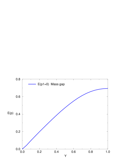
Figure 1: Energy function at $p_{1}=0$, which gives the mass gap for $y\leq 1$, $m_{0}=0.5$.

For $y\geq 1$, one real solution $X$ exists for the momentum in the range $p_{1}\in[p^{c},\pi]$. In figure 2, $E(\pi)$ is shown as a function of $1/y$. Furthermore, there is a negative real solution such that $X\leq-1$ for each $p_{1}\in[0,\pi]$, which corresponds to the time doubler. In this case, we define the energy function as $E(p_{1})\equiv\cosh^{-1}(-X)$. For $p_{1}=0$ and $p_{1}=\pi$, they are shown also in figure 2. The momentum which gives the minimum of $E(p_{1})$ shifts as $y$ varies. For $m_{0}=0.5$, it shifts from $p^{c}$ to $\pi$ as $y$ increases. Then the mass gap merges finally to $E(\pi)$. It is shown also in figure 2.

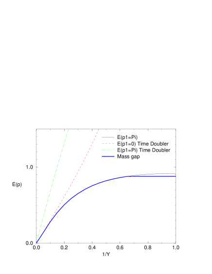
Figure 2: Energy functions of particle at $p_{1}=\pi$ and time-doublers at $p_{1}=0,\pi$ for $y\geq 1$, $m_{0}=0.5$. The mass gap is also shown.

Consistently to the previous discussion about the limits $y=0$ or $y=\infty$, the mass gap of $S_{-}^{v}(n-m;Y)$ becomes small and finally vanishes as the Yukawa coupling becomes close to those limits.

What actually happens in the limits $y=0$ and $y=\infty$ is worth noting. As clearly seen in Eq. (6.70), the wavefunction renormalization constant of one of the chiral components of the massive correlation functions vanishes and that component ceases to propagate at the same time the mass gap vanishes. In this way, at $y=0$ and $y=\infty$, there emerge the massless fermions with the chiralities which match vector-likely with the chirality of the massless Weyl fermion appearing in the overlap correlation function. That vanishing component is naturally understood to live in the opposite side of the waveguide boundary. At finite $y$, this is the chiral partner to form massive states. It has the same transformation property under the chiral $SU(2)$ and there is no symmetry which forbids the massive states.

Since the mass gap remains finite for a nonzero finite $y$, by tuning $\lambda$ close to its critical point, we can always find the region where the perturbation expansion by $\lambda$, Eq. (6.3.2), is a good approximation to the boundary correlation functions. The combolutions of $S_{-}^{v}(n-m;Y)$ with the correlation function of the gauge freedom in there also has the finite correlation lengths. Therefore even inside of the symmetric phase off the critical point, there emerges no massless particle in the boundary correlation functions. Again, there is no symmetry against this fact.

6.4 Expansion in $y$ or $1/y$

Finally, we clarify the structure of the expansions in terms of $y$ and $1/y$. First we examine at the criticality. As we can see in Eq. (6.70), the expansion in terms of $y$ actually means the expansion in terms of the factor

$$y^{2}\frac{\lambda_{-}+m_{0}-B(p)}{\lambda_{-}-m_{0}+B(p)}.$$ (6.84)

However, it is never a small number for $p_{\mu}\simeq(0,0)$, the expansion breaks down for this region. And in this very region, the massless pole would appear in the limit $y=0$. In the case of the expansion in terms of $1/y$, the factor turns out to be

$$\frac{1}{y^{2}}\frac{\lambda_{-}-m_{0}+B(p)}{\lambda_{-}+m_{0}-B(p)}.$$ (6.85)

It is never a small number for $p_{\mu}\simeq(\pi,0),(0,\pi),(\pi,\pi)$. In these regions, the massless poles would appear in the limit $y=\infty$.

For a generic $\lambda$, as we can see in Eq. (6.3.1), the expansion in terms of $y$ means the expansion in terms of the operator in momentum space:

$$\sum_{r,l,p_{t}}y^{2}\frac{1}{C^{\dagger}(p_{s})}\,e^{-ip_{s}r}\left(g_{r}{}_{s}^{t}\right)e^{ip_{t}r}\frac{\left(B(p_{t})-m_{0}-\lambda_{-}(p_{t})\right)}{C(p_{t})}\times$$

$$\quad\qquad\qquad e^{-ip_{t}l}\left(g_{l}^{\dagger}{}_{t}^{i}\right)e^{iql}\left(B(p)-m_{0}-\lambda_{-}(p)\right).$$ (6.86)

However, this operator is not bounded. For a generic configuration of the gauge freedom, it diverges at $p_{s\mu}=(0,0)$. Similarly, as we can see in Eq. (6.3.1), the expansion in terms of $1/y$ means the expansion in terms of the operator in momentum space:

$$\sum_{r,l,p_{t}}\frac{1}{y^{2}}\frac{1}{\left(B(p_{s})-m_{0}-\lambda_{-}(p_{s})\right)}e^{-ip_{s}r}\left(g_{r}{}_{s}^{t}\right)e^{ip_{t}r}\times$$

$$\quad\qquad\frac{C(p_{t})}{\left(B(p_{t})-m_{0}-\lambda_{-}(p_{t})\right)}e^{-ip_{t}l}\left(g_{l}^{\dagger}{}_{t}^{i}\right)e^{ipl}C^{\dagger}(p).$$ (6.87)

This operator is also not bounded. For it diverges at $p_{s\mu}=(\pi,0)$, $(0,\pi)$ and $(\pi,\pi)$.

Therefore, the expansions in terms of $y$ and $1/y$ break down in the very momentum regions where the massless poles would appear in the limits $y=0$ and $y=\infty$. This seems simply because the correlation function actually has a mass gap and the expansion in terms of $y$ or $1/y$ means the expansion in terms of the mass gap. Such expansion is valid only for momenta larger than the mass. Therefore, we find it hard to claim by these expansions that the massless poles at $y=0$ and $y=\infty$ persist for nonzero finite $y$.

7 Summary and Discussion

In summary, we have argued that the two requirements for the pure gauge limit can be fulfilled in the vacuum overlap formulation of a two-dimensional nonabelian chiral gauge theory. These requirements are stated as

1. Mass for the gauge freedom large compared to the physical scale.

2. No physically meaningful light spectrum in boundary correlation functions.

In a two-dimensional $SU(2)$ nonablelian chiral gauge theory, it is naturally expected that the gauge freedom acquires mass dynamically, because of its two-dimensional and nonabelian nature. To make it explicit, we have introduced an asymptotically free self-coupling for the gauge freedom by hand at first. We have examined the boundary correlation functions with the help of the asymptotic freedom and have found that any other light particle does not emerge there. Then we have discussed how far the mass of the gauge freedom can be lifted without affecting the spectrum in the boundary correlation functions. In this respect, we have pointed out two facts. There is no symmetry against the spectrum mass gap of the boundary correlation functions. The IR fixed point due to the Wess-Zumino term is absent in the anomaly free theory.

In fact, we have examined several kinds of the boundary correlation functions. They all have the two-component structure like the correlation function of the two-dimensional Dirac fermion. They are all invariant under the chiral $SU(2)$ global symmetry. There is no symmetry against the mass gap in the spectrum of these correlation functions. What we have found is that it is hard to find the massless fermion in the correlation function from which the gauge degree of freedom does not decouple by some special reasons. The gauge freedom does not decouple in general from the boundary correlation functions. Only when $y=0$ and $y=\infty$, that is, when some special boundary conditions are imposed, it happens and the massless Weyl fermion can emerge there. Otherwise, they consist of vector-like massive states. This observation reminds us about the statement of the Nielsen-Ninomiya theorem extended to the case of interacting theory by Shamir[27], although it might not apply directly to these correlation functions of nonlocal construction of the vacuum overlap.

In clear contrast, the decoupling happens in the overlap correlation functions as shown in [15]. There the correct number of free Weyl fermions emerge. The global symmetry of the overlap correlation functions naturally fits the representation of the Weyl fermions in the target theory. The appearance of poles of species doublers are suppressed by the appearance of zeros at the vanishing momenta for doublers. This has been pointed out to be a possible way out of the Nielsen-Ninomiya theorem[26, 27]. Therefore, this decoupling of the gauge freedom can be regarded as a remarkable property of the definition of the fermion correlation function in the vacuum overlap formulation. It is quite parallel to the situation of the pure gauge limit of the lattice QCD, although the mechanism to suppress the species doublers are very different.

As for the zeros to suppress the species doublers, however, the examples are known in which they cause ghost states which contribute to the vacuum polarization with wrong signature and lead to the wrong normalization[28, 29]. In the case of the vacuum overlap formulation, it has been shown that the perturbative calculation gives the correct normalization of the vacuum polarization[30, 31, 32]. This result is naturally understood from the point of view of the infinite number of the Pauli-Villars fields[33]. It is still desirable to clarify this point in relation to the Ward identity[29].

The free Weyl fermions which emerge in the pure gauge limit do not carry the color indices and does not transform under the global gauge transformation. They are so-called “neutral” fermions in the context of the Wilson-Yukawa model. In this context, the coupling of these “neutral” fermions to the vector bosons, which is also gauge singlet, have been discussed and its triviality was argued[35]. This is one of the reasons why the Wilson-Yukawa formulation is not considered to be able to describe the chiral gauge theory. This argument, however, highly depends on the dimensions and the dynamical nature of the gauge freedom. For example, in two-dimensions, the field variable $g_{n}$ of the gauge freedom has dimension zero if it has the self-coupling term which we considered. In this case, this argument does not lead to the triviality[36]. In four dimensions, if we would consider the higher-derivative coupling for the gauge freedom as introduced in [37], the dimension could differ from unity and the argument does not seem to lead straightforwardly to the triviality. Moreover, there is a general question about the physical relevance of this kind of coupling. Therefore we will leave this issue for future study and will discuss in more detail elsewhere.

We should also mention about the mean field approximation in the context of the vacuum overlap formulation. This approximation replaces the configuration of the gauge freedom by a constant field,

$$g_{n}{}_{i}^{j}=v\delta_{i}^{j},\quad g^{\dagger}_{n}{}_{i}^{j}=v\delta_{i}^{j}.$$ (7.1)

If we do this replacement rather naively in the vacuum overlap formulation, then it turns out that the (null) Wess-Zumino action vanishes and there remains no dependence on $v$ in the fermion sector. Then we cannot get any information about the anomaly. This is why we did not discuss with this approximation.

In the two-dimensional $U(1)$ case, however, the Wess-Zumino term does not exist. Reflecting this fact, the gauge dependence drops out from the fermion determinant in the vacuum overlap formulation[15]. The gauge freedom still couples to the boundary correlation functions. If we examine them by the mean field approximation, we find that the dependence on $v$ also drops out, except for the overall normalizations. See Eqs. (6.3), (6.3), (6.3) and also Eq. (2.3.1). This result means that the mass gap in the boundary correlation function does not depend on the vacuum expectation value. The proportionality relation between the fermion mass and the vacuum expectation value, $m=y\,v$, does not hold even in the broken phase. This might help us to understand what happens in the two-dimensional $U(1)$ theory. However, there is still a serious question about this procedure, because the dependence of the boundary correlation functions on the field variable of the gauge freedom is nonlocal.

Appendix

In the following appendixes, we describe in some detail the evaluations of the formula discussed in the main text. In equations, we implicitly mean sum or integration over the repeated indices or momentum variables. For the momentum integration, the measure is taken as $\frac{d^{2}p}{(2\pi)^{2}}$. We follow closely the second-quantized formulation given in [31].

Appendix A Eigenvectors of free Hamiltonians

In this appendix, we give explicit formula of the eigenvectors of the free Hamiltonians of the three-dimensional Wilson fermions with negative and positive masses. The free Hamiltonians are defined by

$$H_{-nmi}^{\phantom{+nm}j}=\int\frac{d^{2}p}{(2\pi)^{2}}\,e^{ip(n-m)}\left(\begin{array}[]{cc}B(p)-m_{0}&i\sigma_{\mu}\sin p_{\mu}\\ -i\sigma_{\mu}^{\ast}\sin p_{\mu}&-B(p)+m_{0}\end{array}\right)\delta_{i}^{j},$$ (A.1)

$$H_{+nmi}^{\phantom{-nm}j}=\int\frac{d^{2}p}{(2\pi)^{2}}\,e^{ip(n-m)}\left(\begin{array}[]{cc}B(p)+m_{0}&i\sigma_{\mu}\sin p_{\mu}\\ -i\sigma_{\mu}^{\ast}\sin p_{\mu}&-B(p)-m_{0}\end{array}\right)\delta_{i}^{j},$$ (A.2)

where

$$C(p)\equiv i\sigma_{\mu}\sin p_{\mu},\quad B(p)\equiv\sum_{\mu}(1-\cos p_{\mu}).$$ (A.3)

The eigenvectors are obtained as follows:

$$u_{-}(p){}_{i}^{k} = \delta_{i}^{k}\left(\begin{array}[]{c}C(p)\\ -B(p)+m_{0}+\lambda_{-}\end{array}\right)\frac{1}{\sqrt{2\lambda_{-}(\lambda_{-}+m_{0}-B(p))}},$$ (A.6)

$$v_{-}(p){}_{i}^{k} = \delta_{i}^{k}\left(\begin{array}[]{c}B(p)-m_{0}-\lambda_{-}\\ C^{\dagger}(p)\end{array}\right)\frac{1}{\sqrt{2\lambda_{-}(\lambda_{-}+m_{0}-B(p))}},$$ (A.9)

$$u_{+}(p){}_{i}^{k} = \delta_{i}^{k}\left(\begin{array}[]{c}B(p)+m_{0}+\lambda_{+}\\ C^{\dagger}(p)\end{array}\right)\frac{1}{\sqrt{2\lambda_{+}(\lambda_{+}+m_{0}+B(p))}},$$ (A.12)

$$v_{+}(p){}_{i}^{k} = \delta_{i}^{k}\left(\begin{array}[]{c}C(p)\\ -B(p)-m_{0}-\lambda_{+}\end{array}\right)\frac{1}{\sqrt{2\lambda_{+}(\lambda_{+}+m_{0}+B(p))}},$$ (A.15)

where

$$\lambda_{-}\equiv\sqrt{C(p)C^{\dagger}(p)+(B(p)-m_{0})^{2}},$$ (A.16)

$$\lambda_{+}\equiv\sqrt{C(p)C^{\dagger}(p)+(B(p)+m_{0})^{2}}.$$ (A.17)

Appendix B Vacua of the second-quantized Hamiltonians

In this appendix, we give the vacuum of the second-quantized Hamiltonian theory of the free three-dimensional Wilson fermion with negative and positive masses. The defining creation and annihilation operators satisfy the following commutation relations.

$$\left\{\hat{a}_{ni},\hat{a}^{\dagger}_{m}{}^{j}\right\} = \delta_{nm}\delta_{ij},$$ (B.1)

$$\left\{\hat{a}_{ni},\hat{a}_{mj}\right\} = 0,$$ (B.2)

$$\left\{\hat{a}^{\dagger}_{n}{}^{i},\hat{a}^{\dagger}_{m}{}^{j}\right\} = 0.$$ (B.3)

The Fock space is constructed on the auxiliary vacuum $|0\rangle$ defined by

$$\hat{a}_{n}{}_{i}|0\rangle=0.$$ (B.5)

The second quantized Hamiltonian $\hat{H}_{+}$ is diagonalized by the creation and annihilation operators defined as follows:

$$\hat{b}_{+}(p){}_{k} = u^{\dagger}_{+}(p){}_{k}^{i}e^{-ipm}\hat{a}_{m}{}_{i},$$ (B.6)

$$\hat{b}_{+}^{\dagger}(p){}^{k} = \hat{a}_{n}^{\dagger}{}^{i}e^{ipn}u_{+}(p){}_{i}^{k},$$ (B.7)

$$\hat{d}_{+}(p){}^{k} = \hat{a}_{n}^{\dagger}{}^{i}e^{ipn}v_{+}(p){}_{i}^{k},$$ (B.8)

$$\hat{d}_{+}^{\dagger}(p){}_{k} = v^{\dagger}_{+}(p){}^{i}_{k}e^{-ipm}\hat{a}_{m}{}_{i},$$ (B.9)

$$\hat{a}_{n}^{\dagger}{}^{i}H_{+nm}{}_{i}^{j}\hat{a}_{m}{}_{j} = \int\frac{d^{2}p}{(2\pi)^{2}}\sum_{k}\,\left[\left(\hat{a}_{n}^{\dagger}{}^{i}e^{ipn}u_{+}(p){}_{i}^{k}\right)\lambda_{+}(p)\left(u^{\dagger}_{+}(p){}^{j}_{k}e^{-ipm}\hat{a}_{m}{}_{j}\right)\right.$$

$$\qquad\qquad\qquad\left.-\left(\hat{a}_{n}^{\dagger}{}^{i}e^{ipn}v_{+}(p){}_{i}^{k}\right)\lambda_{+}(p)\left(v^{\dagger}_{+}(p){}^{j}_{k}e^{-ipm}\hat{a}_{m}{}_{j}\right)\right]$$

$$= \int\frac{d^{2}p}{(2\pi)^{2}}\sum_{k}\,\left[\hat{b}_{+}^{\dagger}(p){}^{k}\lambda_{+}(p)\hat{b}_{+}(p){}_{k}-\hat{d}_{+}(p){}^{k}\lambda_{+}(p)\hat{d}_{+}^{\dagger}(p){}_{k}\right].$$

Similarly, the second quantized Hamiltonian $\hat{H}_{-}$ is diagonalized by the creation and annihilation operators defined as follows:

$$\hat{b}_{-}(p){}_{k} = u^{\dagger}_{-}(p){}_{k}^{i}e^{-ipm}\hat{a}_{m}{}_{i},$$ (B.11)

$$\hat{b}_{-}^{\dagger}(p){}^{k} = \hat{a}_{n}^{\dagger}{}^{i}e^{ipn}u_{-}(p){}_{i}^{k},$$ (B.12)

$$\hat{d}_{-}(p){}^{k} = \hat{a}_{n}^{\dagger}{}^{i}e^{ipn}v_{-}(p){}_{i}^{k},$$ (B.13)

$$\hat{d}_{-}^{\dagger}(p){}_{k} = v^{\dagger}_{-}(p){}^{i}_{k}e^{-ipm}\hat{a}_{m}{}_{i},$$ (B.14)

$$\hat{a}_{n}^{\dagger}{}^{i}H_{-nm}{}_{i}^{j}\hat{a}_{m}{}_{j} = \int\frac{d^{2}p}{(2\pi)^{2}}\sum_{k}\,\left[\left(\hat{a}_{n}^{\dagger}{}^{i}e^{ipn}u_{-}(p){}_{i}^{k}\right)\lambda_{-}(p)\left(u^{\dagger}_{-}(p){}^{j}_{k}e^{-ipm}\hat{a}_{m}{}_{j}\right)\right.$$

$$\qquad\qquad\qquad\left.-\left(\hat{a}_{n}^{\dagger}{}^{i}e^{ipn}v_{-}(p){}_{i}^{k}\right)\lambda_{-}(p)\left(v^{\dagger}_{-}(p){}^{j}_{k}e^{-ipm}\hat{a}_{m}{}_{j}\right)\right]$$

$$= \int\frac{d^{2}p}{(2\pi)^{2}}\sum_{k}\,\left[\hat{b}_{-}^{\dagger}(p){}^{k}\lambda_{-}(p)\hat{b}_{-}(p){}_{k}-\hat{d}_{-}(p){}^{k}\lambda_{-}(p)\hat{d}_{-}^{\dagger}(p){}_{k}\right].$$

These creation and annihilation operators satisfy the following commutation relations.

$$\left\{\hat{b}_{+}(p){}_{k},\hat{b}_{+}^{\dagger}(q){}^{l}\right\} = (2\pi)^{2}\delta^{2}(p-q)\delta_{k}^{l},$$ (B.16)

$$\left\{\hat{d}_{+}(p){}^{k},\hat{d}_{+}^{\dagger}(q){}_{l}\right\} = (2\pi)^{2}\delta^{2}(p-q)\delta^{k}_{l},$$ (B.17)

$$\left\{\hat{b}_{+}(p){}_{k},\hat{d}_{+}(q){}^{l}\right\} = 0,$$ (B.18)

$$\left\{\hat{b}_{+}^{\dagger}(p){}^{k},\hat{d}_{+}^{\dagger}(q){}_{l}\right\} = 0.$$ (B.19)

$$\left\{\hat{b}_{-}(p){}_{k},\hat{b}_{-}^{\dagger}(q){}^{l}\right\} = (2\pi)^{2}\delta^{2}(p-q)\delta_{k}^{l},$$ (B.20)

$$\left\{\hat{d}_{-}(p){}^{k},\hat{d}_{-}^{\dagger}(q){}_{l}\right\} = (2\pi)^{2}\delta^{2}(p-q)\delta^{k}_{l},$$ (B.21)

$$\left\{\hat{b}_{-}(p){}_{k},\hat{d}_{-}(q){}^{l}\right\} = 0,$$ (B.22)

$$\left\{\hat{b}_{-}^{\dagger}(p){}^{k},\hat{d}_{-}^{\dagger}(q){}_{l}\right\} = 0.$$ (B.23)

$$\left\{\hat{b}_{-}(p){}_{k},\hat{b}_{+}^{\dagger}(q){}^{l}\right\} = (2\pi)^{2}\delta^{2}(p-q)u^{\dagger}_{-}(p)u_{+}(p)\delta_{k}^{l},$$ (B.24)

$$\left\{\hat{b}^{\dagger}_{-}(p){}^{k},\hat{b}_{+}(q){}_{l}\right\} = (2\pi)^{2}\delta^{2}(p-q)u^{\dagger}_{+}(p)u_{-}(p)\delta^{k}_{l},$$ (B.25)

$$\left\{\hat{d}_{-}(p){}^{k},\hat{d}_{+}^{\dagger}(q){}_{l}\right\} = (2\pi)^{2}\delta^{2}(p-q)v^{\dagger}_{+}(p)v_{-}(p)\delta^{k}_{l},$$ (B.26)

$$\left\{\hat{d}^{\dagger}_{-}(p){}_{k},\hat{d}_{+}(q){}^{l}\right\} = (2\pi)^{2}\delta^{2}(p-q)v^{\dagger}_{-}(p)v_{+}(p)\delta_{k}^{l},$$ (B.27)

$$\left\{\hat{b}_{-}(p){}_{k},\hat{d}_{+}(q){}^{l}\right\} = (2\pi)^{2}\delta^{2}(p-q)u^{\dagger}_{-}(p)v_{+}(p)\delta_{k}^{l},$$ (B.28)

$$\left\{\hat{b}_{-}^{\dagger}(p){}^{k},\hat{d}_{+}^{\dagger}(q){}_{l}\right\} = (2\pi)^{2}\delta^{2}(p-q)v^{\dagger}_{+}(p)u_{-}(p)\delta^{k}_{l},$$ (B.29)

$$\left\{\hat{b}_{+}(p){}_{k},\hat{d}_{-}(q){}^{l}\right\} = (2\pi)^{2}\delta^{2}(p-q)u^{\dagger}_{+}(p)v_{-}(p)\delta_{k}^{l},$$ (B.30)

$$\left\{\hat{b}_{+}^{\dagger}(p){}^{k},\hat{d}_{-}^{\dagger}(q){}_{l}\right\} = (2\pi)^{2}\delta^{2}(p-q)v^{\dagger}_{-}(p)u_{+}(p)\delta^{k}_{l}.$$ (B.31)

Vacua of the second-quantized Hamiltonians are given by

$$|+\rangle=\prod_{p,k}\hat{d}_{+}(p){}^{k}|0\rangle,$$ (B.32)

$$|-\rangle=\prod_{p,k}\hat{d}_{-}(p){}^{k}|0\rangle.$$ (B.33)

The defining creation and annihilation operators are expanded by the creation and annihilation operators in the diagonalized bases as follows:

$$\hat{a}_{n}{}_{i} = \int\frac{d^{2}p}{(2\pi)^{2}}e^{ipn}\left[u_{+}(p)\hat{b}_{+}(p){}_{i}+v_{+}(p)\hat{d}^{\dagger}_{+}(p){}_{i}\right]$$ (B.34)

$$= \int\frac{d^{2}p}{(2\pi)^{2}}e^{ipn}\left[u_{-}(p)\hat{b}_{-}(p){}_{i}+v_{-}(p)\hat{d}^{\dagger}_{-}(p){}_{i}\right],$$ (B.35)

$$\hat{a}^{\dagger}_{n}{}^{i} = \int\frac{d^{2}p}{(2\pi)^{2}}e^{-ipn}\left[u^{\dagger}_{+}(p)\hat{b}^{\dagger}_{+}(p){}^{i}+v^{\dagger}_{+}(p)\hat{d}_{+}(p){}^{i}\right]$$ (B.36)

$$= \int\frac{d^{2}p}{(2\pi)^{2}}e^{-ipn}\left[u^{\dagger}_{-}(p)\hat{b}^{\dagger}_{-}(p){}^{i}+v^{\dagger}_{-}(p)\hat{d}_{-}(p){}^{i}\right].$$ (B.37)

Appendix C Vacua in pure gauge limit

In this appendix, we give the vacuum of the second-quantized Hamiltonian theory of the three-dimensional Wilson fermion with negative mass in the pure gauge limit. The positive mass case can be formulated in a similar manner. In the pure gauge limit, the interacting second-quantized Hamiltonian with the negative mass can be written as follows:

$$\hat{H}_{+}\left[g_{n}g^{\dagger}_{n+\hat{\mu}}\right]=\hat{G}\hat{H}_{+}\hat{G}^{\dagger},\quad(\beta=0),$$ (C.1)

where $\hat{G}$ is the operator of gauge transformation defined by

$$\hat{G}=\exp\left(\sum_{n}\hat{a}_{n}^{\dagger i}\{\log g_{n}\}_{i}{}^{j}\hat{a}_{nj}\right).$$ (C.2)

Accordingly, the vacuum in the pure gauge limit can be expressed as

$$\hat{G}|+\rangle.$$ (C.3)

The Hamiltonian in the pure gauge limit can be diagonalized by the following creation and annihilation operators.

$$\hat{G}|+\rangle=\prod_{p,k}\hat{d}{}^{G}_{+}(p){}^{k}|0\rangle.$$ (C.4)

$$\hat{b}^{G}_{+}(p){}_{k} = u^{\dagger}_{+}(p){}_{k}^{i}e^{-ipm}\left(g_{m}^{\dagger}{}_{i}^{j}\right)\hat{a}_{m}{}_{j}.$$ (C.5)

$$\hat{b}_{+}^{G\dagger}(p){}^{k} = \hat{a}_{n}^{\dagger}{}^{i}\left(g_{n}{}_{i}^{j}\right)e^{ipn}u_{+}(p){}_{j}^{k}.$$ (C.6)

$$\hat{d}^{G}_{+}(p){}^{k} = \hat{a}_{n}^{\dagger}{}^{i}\left(g_{n}{}_{i}^{j}\right)e^{ipn}v_{+}(p){}_{j}^{k}.$$ (C.7)

$$\hat{d}_{+}^{G\dagger}(p){}_{k} = v^{\dagger}_{+}(p){}^{i}_{k}e^{-ipm}\left(g_{m}^{\dagger}{}_{i}^{j}\right)\hat{a}_{m}{}_{j}.$$ (C.8)

They satisfy the following commutation relations.

$$\left\{\hat{b}^{G}_{+}(p){}_{k},\hat{b}_{+}^{G\dagger}(q){}^{l}\right\} = (2\pi)^{2}\delta^{2}(p-q)\delta_{k}^{l}.$$ (C.9)

$$\left\{\hat{d}^{G}_{+}(p){}^{k},\hat{d}_{+}^{G\dagger}(q){}_{l}\right\} = (2\pi)^{2}\delta^{2}(p-q)\delta^{k}_{l}.$$ (C.10)

$$\left\{\hat{b}^{G}_{+}(p){}_{k},\hat{d}^{G}_{+}(q){}^{l}\right\} = 0.$$ (C.11)

$$\left\{\hat{b}_{+}^{G\dagger}(p){}^{k},\hat{d}_{+}^{G\dagger}(q){}_{l}\right\} = 0.$$ (C.12)

$$\left\{\hat{b}_{+}(p){}_{k},\hat{b}_{+}^{G\dagger}(q){}^{l}\right\} = u^{\dagger}_{+}(p){}_{k}^{i}e^{-ipm}\left(g_{m}{}_{i}^{j}\right)e^{iqm}u_{+}(q){}_{j}^{l}.$$ (C.13)

$$\left\{\hat{d}_{+}(p){}^{k},\hat{d}_{+}^{G\dagger}(q){}_{l}\right\} = v^{\dagger}_{+}(q){}^{i}_{l}e^{-iqm}\left(g_{m}^{\dagger}{}_{i}^{j}\right)e^{ipm}v_{+}(p){}_{j}^{k}.$$ (C.14)

$$\left\{\hat{b}_{+}(p){}_{k},\hat{d}^{G}_{+}(q){}^{l}\right\} = u^{\dagger}_{+}(p){}_{k}^{i}e^{-ipm}\left(g_{m}{}_{i}^{j}\right)e^{iqm}v_{+}(q){}_{j}^{l}.$$ (C.15)

$$\left\{\hat{b}^{G}_{+}(p){}_{k},\hat{d}_{+}(q){}^{l}\right\} = u^{\dagger}_{+}(p){}_{k}^{i}e^{-ipm}\left(g_{m}^{\dagger}{}_{i}^{j}\right)e^{iqm}v_{+}(q){}_{j}^{l}.$$ (C.16)

$$\left\{\hat{b}_{+}^{\dagger}(p){}^{k},\hat{d}_{+}^{G\dagger}(q){}_{l}\right\} = v^{\dagger}_{+}(q){}^{i}_{l}e^{-iqm}\left(g_{m}^{\dagger}{}_{i}^{j}\right)e^{ipm}u_{+}(p){}_{j}^{k}.$$ (C.17)

$$\left\{\hat{b}_{+}^{G\dagger}(p){}^{k},\hat{d}_{+}^{\dagger}(q){}_{l}\right\} = v^{\dagger}_{+}(q){}^{i}_{l}e^{-ipm}\left(g_{m}{}_{i}^{j}\right)e^{ipm}u_{+}(p){}_{j}^{k}.$$ (C.18)

In this diagonalizing basis in the pure gauge limit, the defining creation and annihilation operators are expanded as

$$\hat{a}_{n}{}_{i} = \int\frac{d^{2}p}{(2\pi)^{2}}\left(g_{n}{}_{i}^{k}\right)e^{ipn}\left[u_{+}(p)\hat{b}^{G}_{+}(p){}_{k}+v_{+}(p)\hat{d}^{G\dagger}_{+}(p){}_{k}\right],$$ (C.19)

$$\hat{a}^{\dagger}_{n}{}^{i} = \int\frac{d^{2}p}{(2\pi)^{2}}\left[\hat{b}^{G\dagger}_{+}(p){}^{k}u^{\dagger}_{+}(p)+\hat{d}^{G}_{+}(p){}^{k}v^{\dagger}_{+}(p)\right]e^{-ipn}\left(g^{\dagger}_{n}{}_{k}^{i}\right).$$ (C.20)

A similar formulation is possible for the case of the Hamiltonian with positive mass.

Appendix D Action of Yukawa Coupling Operator

In this appendix, we give the definition of the operator of the boundary Yukawa coupling and its action. The Yukawa coupling at the waveguide boundary[11] can be expressed by the following operator[18] inserted in the overlaps which implements the Wigner-Brillouin phase convention.

$$\hat{Y} = \exp\left(\sum_{n,i}\ln y\,(\hat{a}_{n1}^{\dagger}{}^{i}\hat{a}_{n1}{}_{i}-\hat{a}_{n2}^{\dagger}{}^{i}\hat{a}_{n2}{}_{i})\right)$$ (D.1)

$$= \prod_{ni}\left(\hat{a}_{n1}{}_{i}\hat{a}_{n1}^{\dagger}{}^{i}+y\hat{a}_{n1}^{\dagger}{}^{i}\hat{a}_{n1}{}_{i}\right)\left(\hat{a}_{n2}{}_{i}\hat{a}_{n2}^{\dagger}{}^{i}+\frac{1}{y}\hat{a}_{n2}^{\dagger}{}^{i}\hat{a}_{n2}{}_{i}\right).$$

This Yukawa coupling operator acts on the vacua in the following manner:

$$\hat{Y}|+\rangle = \prod_{p,k}\left(\hat{a}_{n}^{\dagger}{}^{i}e^{ipn}Yv_{+}(p){}_{i}^{k}\right)|0\rangle$$ (D.2)

$$= \prod_{p,k}\left(\hat{b}^{\dagger}_{+}(p){}^{k}u^{\dagger}_{+}(p)Yv_{+}(p)+\hat{d}_{+}(p){}^{k}v^{\dagger}_{+}(p)Yv_{+}(p)\right)|0\rangle,$$

$$\hat{Y}|-\rangle = \prod_{p,k}\left(\hat{a}_{n}^{\dagger}{}^{i}e^{ipn}Yv_{-}(p){}_{i}^{k}\right)|0\rangle$$ (D.3)

$$= \prod_{p,k}\left(\hat{b}^{\dagger}_{-}(p){}^{k}u^{\dagger}_{-}(p)Yv_{-}(p)+\hat{d}_{-}(p){}^{k}v^{\dagger}_{-}(p)Yv_{-}(p)\right)|0\rangle,$$

where $Y$ is the matrix in the spinor space given by

$$Y=\left(\begin{array}[]{cc}y&0\\ 0&\frac{1}{y}\end{array}\right)=yP_{R}+\frac{1}{y}P_{L}.$$ (D.4)

Appendix E Calculation of the null Wess-Zumino Action

In this appendix, we describe the perturbative calculation of the null Wess-Zumino action in detail. The defining overlaps of the representation $r$ which implement the Wigner-Brillouin phase convention can be written explicitly with the eigenvectors as follows:

$$\langle-|\hat{G}^{\dagger}\hat{Y}|-\rangle_{r} = \det_{(p,i)(q,j)}\left[\sum_{m}v^{\dagger}_{-}(p)e^{-ipm}\left(g_{m}^{\dagger}{}_{i}^{j}\right)e^{iqm}Yv_{-}(q)\right],$$ (E.1)

$$\langle+|\hat{Y}\hat{G}|+\rangle_{r} = \det_{(p,i)(q,j)}\left[\sum_{m}v^{\dagger}_{+}(p)Ye^{-ipm}\left(g_{m}{}_{i}^{j}\right)e^{iqm}v_{+}(q)\right].$$ (E.2)

Then the explicit formula of the contribution from the fermion in the representation $r$ to the null Wess-Zumino action is given as

$$i\Delta\Gamma_{WZ}[g;Y]_{r} = i{\rm Im}{\rm Tr}\,{\rm Ln}\left[\sum_{m}v^{\dagger}_{-}(p)e^{-ipm}\left(g_{m}^{\dagger}{}_{i}^{j}\right)e^{iqm}Yv_{-}(q)\right]$$

$$+ i{\rm Im}{\rm Tr}\,{\rm Ln}\left[\sum_{m}v^{\dagger}_{+}(p)Ye^{-ipm}\left(g_{m}{}_{i}^{j}\right)e^{iqm}v_{+}(q)\right].$$

In terms of the fluctuation of the gauge freedom,

$$g_{m}^{\dagger}{}_{i}^{j}-{\mathchoice{\rm 1\mskip-4.0mul}{\rm 1\mskip-4.0mul}{\rm 1\mskip-4.5mul}{\rm 1\mskip-5.0mul}}{}_{i}^{j}=-i\lambda\pi{}_{i}^{j}+(-i)^{2}\frac{1}{2!}\lambda^{2}\pi^{2}{}_{i}^{j}+(-i)^{3}\frac{1}{3!}\lambda^{3}\pi^{3}{}_{i}^{j}+\cdots,$$ (E.4)

$$\pi{}_{i}^{j}\equiv\pi^{a}T^{a}{}_{i}^{k}.$$ (E.5)

the defining overlap with negative mass can be expanded as follows:

$${\rm Tr}\,{\rm Ln}\left[\sum_{m}v^{\dagger}_{-}(p)e^{-ipm}\left(g_{m}^{\dagger}{}_{i}^{j}\right)e^{iqm}Yv_{-}(q)\right]$$

$$={\rm Tr}\,{\rm Ln}\left[v^{\dagger}_{-}(p)Yv_{-}(p)(2\pi)^{2}\delta^{2}(p-q)\left({\mathchoice{\rm 1\mskip-4.0mul}{\rm 1\mskip-4.0mul}{\rm 1\mskip-4.5mul}{\rm 1\mskip-5.0mul}}{}_{i}^{j}\right)\right.$$

$$\qquad\qquad\left.+\sum_{m}v^{\dagger}_{-}(p)e^{-ipm}\left(g_{m}^{\dagger}{}_{i}^{j}-{\mathchoice{\rm 1\mskip-4.0mul}{\rm 1\mskip-4.0mul}{\rm 1\mskip-4.5mul}{\rm 1\mskip-5.0mul}}{}_{i}^{j}\right)e^{iqm}Yv_{-}(q)\right]$$

$$={\rm Tr}\,{\rm Ln}\left[v^{\dagger}_{-}(p)Yv_{-}(p)(2\pi)^{2}\delta^{2}(p-q)\left({\mathchoice{\rm 1\mskip-4.0mul}{\rm 1\mskip-4.0mul}{\rm 1\mskip-4.5mul}{\rm 1\mskip-5.0mul}}{}_{i}^{j}\right)\right]$$

$$+{\rm Tr}\,{\rm Ln}\left[(2\pi)^{2}\delta^{2}(p-q)\left({\mathchoice{\rm 1\mskip-4.0mul}{\rm 1\mskip-4.0mul}{\rm 1\mskip-4.5mul}{\rm 1\mskip-5.0mul}}{}_{i}^{j}\right)\right.$$

$$\qquad\qquad\left.+\frac{1}{v^{\dagger}_{-}(p)Yv_{-}(p)}\sum_{m}v^{\dagger}_{-}(p)e^{-ipm}\left(g_{m}^{\dagger}{}_{i}^{j}-{\mathchoice{\rm 1\mskip-4.0mul}{\rm 1\mskip-4.0mul}{\rm 1\mskip-4.5mul}{\rm 1\mskip-5.0mul}}{}_{i}^{j}\right)e^{iqm}Yv_{-}(q)\right]$$

$$=\ln\left(\langle-|\hat{Y}|-\rangle\right)$$

$$+{\rm Tr}\,\sum_{l=1}^{\infty}\frac{(-1)^{l-1}}{l}\left[\sum_{m}e^{-ipm}\left(g_{m}^{\dagger}{}_{i}^{j}-{\mathchoice{\rm 1\mskip-4.0mul}{\rm 1\mskip-4.0mul}{\rm 1\mskip-4.5mul}{\rm 1\mskip-5.0mul}}{}_{i}^{j}\right)e^{iqm}S^{v}_{-}(q;Y)\right]^{l},$$ (E.6)

where

$$S^{v}_{-}(p;Y)\equiv\frac{1}{v^{\dagger}_{-}(p)Yv_{-}(p)}Yv_{-}(p)v^{\dagger}_{-}(p).$$ (E.7)

In the first order term, $l=1$:

$${\rm Tr}\,\left[\sum_{m}e^{-ipm}\left(g_{m}^{\dagger}{}_{i}^{j}-{\mathchoice{\rm 1\mskip-4.0mul}{\rm 1\mskip-4.0mul}{\rm 1\mskip-4.5mul}{\rm 1\mskip-5.0mul}}{}_{i}^{j}\right)e^{iqm}S_{-}(q;Y)\right],$$ (E.8)

${\cal O}(\pi)$ vanishes because of ${\rm Tr}(T^{a})=0$. ${\cal O}(\pi^{2})$ is irrelevant because it is real. ${\cal O}(\pi^{3})$ vanishes because of bose symmetry with respect to the three group indices in ${\rm Tr}(T^{a}T^{b}T^{c})$.

In the second order term, $l=2$:

$$-\frac{1}{2}{\rm Tr}\,\left[\sum_{m}e^{-ipm}\left(g_{m}^{\dagger}{}_{i}^{j}-{\mathchoice{\rm 1\mskip-4.0mul}{\rm 1\mskip-4.0mul}{\rm 1\mskip-4.5mul}{\rm 1\mskip-5.0mul}}{}_{i}^{j}\right)e^{iqm}S_{-}(q;Y)\right]^{2},$$ (E.9)

${\cal O}(\pi^{2})$ is irrelevant because it is real. ${\cal O}(\pi^{3})$ vanishes because of bose symmetry with respect to two of the three group indices in ${\rm Tr}(T^{a}T^{b}T^{c})$.

The third order term, $l=3$:

$$\frac{1}{3}{\rm Tr}\,\left[\sum_{m}e^{-ipm}\left(g_{m}^{\dagger}{}_{i}^{j}-{\mathchoice{\rm 1\mskip-4.0mul}{\rm 1\mskip-4.0mul}{\rm 1\mskip-4.5mul}{\rm 1\mskip-5.0mul}}{}_{i}^{j}\right)e^{iqm}S_{-}(q;Y)\right]^{3}$$ (E.10)

has a nontrivial ${\cal O}(\pi^{3})$ contribution to the null Wess-Zumino action, which is evaluated as follows:

$$i\Delta\Gamma_{WZ}[\pi;Y]_{r-}$$

$$=i\frac{1}{3}\lambda^{3}\int\frac{d^{2}p_{1}}{(2\pi)^{2}}\frac{d^{2}p_{2}}{(2\pi)^{2}}\frac{d^{2}p_{3}}{(2\pi)^{2}}(2\pi)^{2}\delta^{2}(p_{1}+p_{2}+p_{3})i\epsilon^{abc}\left(\pi^{a}(p_{1})\pi^{b}(p_{2})\pi^{c}(p_{3})\right)\times$$

$$\qquad\qquad A_{r}\int\frac{d^{2}q}{(2\pi)^{2}}{\rm Tr}\left[S^{v}_{-}(q+p_{1};Y)S^{v}_{-}(q;Y)S^{v}_{-}(q-p_{2};Y)\right]+\cdots,$$ (E.11)

where

$${\rm Tr}\left(T^{a}T^{b}T^{c}\right)_{r}=i\epsilon^{abc}A_{r}.$$ (E.12)

For the anomaly free theory in consideration,

$$\sum_{r}A_{r}=4\times\frac{1}{4}-1=0.$$ (E.13)

The contribution of the defining overlap with positive mass can be also evaluated in a similar manner. Then the induced null Wess-Zumino action vanishes completely up to ${\cal O}(\pi^{3})$. Note that this is true before the expansion with respect to external momenta.

The contribution of each fermion to the null Wess-Zumino action should contain the Wess-Zumino term:

$$\int\frac{d^{2}q}{(2\pi)^{2}}{\rm Tr}\left[S_{-}(q+p_{1};Y)S_{-}(q;Y)S_{-}(q-p_{2};Y)\right] = -\epsilon_{\mu\nu}p_{1\mu}p_{2\nu}c_{WZ}[Y]_{-}+\cdots.$$

The coefficient $c_{WZ}[Y]_{-}$ is given by the following integral:

$$c_{WZ}[Y]_{-} \equiv \frac{1}{2!}\epsilon_{\mu\nu}\int\frac{d^{2}q}{(2\pi)^{2}}{\rm Tr}\left[\partial_{\mu}S^{v}_{-}(q;Y)S^{v}_{-}(q;Y)\partial_{\nu}S^{v}_{-}(q;Y)\right].$$

In order to evaluate this coefficient, let us introduce the following wave function:

$$v_{-}(p;Y)\equiv Y^{1/2}v_{-}(p)=\left(\begin{array}[]{c}y^{1/2}\left(B(p)-m_{0}-\lambda_{-}\right)\\ y^{-1/2}(-i)\sigma^{\ast}_{\mu}C_{\mu}(p)\end{array}\right),$$ (E.16)

where $\sigma_{\mu}=(i,1)$. Using this wave function, the above tree-point vertex can be rewritten as

$${\rm Tr}\left[S_{-}(q+p_{1};Y)S_{-}(q;Y)S_{-}(q-p_{2};Y)\right]$$

$$= \frac{v^{\dagger}_{-}(q+p_{1};Y)v_{-}(q;Y)\,v^{\dagger}_{-}(q;Y)v_{-}(q-p_{2};Y)\,v^{\dagger}_{-}(q-p_{2};Y)v_{-}(q+p_{1};Y)}{v^{\dagger}_{-}(q+p_{1};Y)v_{-}(q+p_{1};Y)\,v^{\dagger}_{-}(q;Y)v_{-}(q;Y)\,v^{\dagger}_{-}(q-p_{2};Y)v_{-}(q-p_{2};Y)}.$$

Then $c_{WZ}[Y]_{-}$ is calculated as

$$c_{WZ}[Y]_{-}$$

$$=\frac{1}{2!}\epsilon_{\mu\nu}\int\frac{d^{2}q}{(2\pi)^{2}}{\rm Tr}\left[\partial_{\mu}S_{-}(q;Y)S_{-}(q;Y)\partial_{\nu}S_{-}(q;Y)\right]$$

$$=\frac{1}{2!}\epsilon_{\mu\nu}\int\frac{d^{2}q}{(2\pi)^{2}}\left\{\frac{\partial_{\nu}v^{\dagger}_{-}(q;Y)\cdot\partial_{\mu}v_{-}(q;Y)}{\left(v^{\dagger}_{-}(q;Y)v_{-}(q;Y)\right)}\right.$$

$$\left.\qquad\qquad\qquad\qquad-\frac{\partial_{\nu}v^{\dagger}_{-}(q;Y)\cdot v_{-}(q;Y)v^{\dagger}_{-}(q;Y)\cdot\partial_{\mu}v_{-}(q;Y)}{\left(v^{\dagger}_{-}(q;Y)v_{-}(q;Y)\right)^{2}}\right\}$$

$$=(-i)\int\frac{d^{2}q}{(2\pi)^{2}}\frac{\left\{(m_{0}-B)\partial_{\mu}C_{\mu}\partial_{\nu}C_{\nu}+\partial_{\mu}C_{\mu}C_{\nu}\partial_{\nu}B+\partial_{\nu}C_{\nu}C_{\mu}\partial_{\mu}B\right\}}{\lambda_{-}\left[y(\lambda_{-}+m_{0}-B)+\frac{1}{y}(\lambda_{-}-m_{0}+B)\right]^{2}}.$$

Furthermore we can show the following relation by the straightforward calculation.

$$c_{WZ}[Y]_{-} = (-i)\frac{1}{2}\int\frac{d^{2}q}{(2\pi)^{2}}\int_{-\infty}^{\infty}\frac{d\omega}{(2\pi)}$$

$$\quad\frac{1}{2!}\epsilon_{\mu\nu}{\rm Tr}\left\{S_{3}(q,\omega;Y)\partial_{\mu}S_{3}^{-1}(q,\omega;Y)\times\right.$$

$$\left.\qquad\qquad S_{3}(q,\omega;Y)\partial_{\nu}S_{3}^{-1}(q,\omega;Y)S_{3}(q,\omega;Y)\partial_{\omega}S_{3}^{-1}(q,\omega;Y)\right\},$$

where

$$S_{3}(p,\omega;Y)$$

$$=\frac{\left\{-i\gamma_{5}\omega-i\gamma_{\mu}C_{\mu}(p)+\frac{1}{2}\left[y(B-m_{0}-\lambda_{-})+\frac{1}{y}(B-m_{0}+\lambda_{-})\right]\right\}}{\omega^{2}+\lambda^{\prime 2}_{-}}.$$

Then, following the method of calculation in [23], we obtain

$$c_{WZ}[Y]_{-}$$

$$=(-i)\frac{1}{2}\frac{1}{4\pi}\sum_{k=0}^{2}(-1)^{k}\left(\begin{array}[]{c}2\\ k\end{array}\right)\frac{m_{k}}{|m_{k}|}\qquad m_{k}=\left\{\begin{array}[]{c}-ym_{0}\quad(k=0)\\ \frac{1}{y}(2k-m_{0})\quad(k\not=0)\end{array}\right.$$ (E.25)

$$=(-i)\frac{1}{4\pi}.$$ (E.26)

By the similar calculation, we find that $c_{WZ}[Y]_{+}$ vanishes. Thus we obtain the correct value of the Wess-Zumino term as far as $y$ is nonzero finite.

In order to deduce the above form of the propagator, Eq. (E), we note the fact that the wavefunction $v_{-}(p;Y)$ can be an eigenvector of a certain Hamiltonian which is generalized to include the boundary Yukawa coupling:

$$v_{-}(p;Y)v^{\dagger}_{-}(p;Y)$$

$$=\frac{1}{y(\lambda_{-}+m_{0}-B)+\frac{1}{y}(\lambda_{-}-m_{0}+B)}\left(\begin{array}[]{cc}y(\lambda_{-}+m_{0}-B)&-C\\ -C^{\dagger}&\frac{1}{y}(\lambda_{-}-m_{0}+B)\end{array}\right)$$ (E.29)

$$\equiv\frac{1}{2}-\frac{1}{2}\frac{H^{\prime}_{-}}{\lambda^{\prime}_{-}}.$$ (E.30)

Then the Hamiltonian and the eigenvalue can be determined up to the overall factor.

$$H^{\prime}_{-}(p;Y)\equiv\gamma_{5}\left\{i\gamma_{\mu}C_{\mu}(p)+\frac{1}{2}\left[y(B-m_{0}-\lambda_{-})+\frac{1}{y}(B-m_{0}+\lambda_{-})\right]\right\},$$

(E.31)

$$\lambda^{\prime}_{-}\equiv\frac{1}{2}\left[y(\lambda_{-}+m_{0}-B)+\frac{1}{y}(\lambda_{-}-m_{0}+B)\right].$$ (E.32)

A Dirac operator can be constructed from this Hamiltonian,

$$D_{3}(p,\omega;Y) \equiv i\gamma_{5}\omega+\gamma_{5}H^{\prime}_{-}(p;Y)$$

$$=i\gamma_{5}\omega+i\gamma_{\mu}C_{\mu}(p)+\frac{1}{2}\left[y(B-m_{0}-\lambda_{-})+\frac{1}{y}(B-m_{0}+\lambda_{-})\right].$$

This Dirac operator satisfies the following relation,

$$D_{3}(p,\omega;Y)D^{\dagger}_{3}(p,\omega;Y)$$

$$=\omega^{2}+C_{\mu}^{2}(p)+\frac{1}{4}\left[y(B-m_{0}-\lambda_{-})+\frac{1}{y}(B-m_{0}+\lambda_{-})\right]^{2}$$

$$=\omega^{2}+(\lambda_{-}+m_{0}-B)(\lambda_{-}-m_{0}+B)$$

$$+\frac{1}{4}\left[y^{2}(B-m_{0}-\lambda_{-})^{2}+\frac{1}{y^{2}}(B-m_{0}+\lambda_{-})^{2}-2(B-m_{0}-\lambda_{-})(B-m_{0}+\lambda_{-})\right]$$

$$=\omega^{2}+\frac{1}{4}\left[y^{2}(B-m_{0}-\lambda_{-})^{2}+\frac{1}{y^{2}}(B-m_{0}+\lambda_{-})^{2}+2(B-m_{0}-\lambda_{-})(B-m_{0}+\lambda_{-})\right]$$

$$=\omega^{2}+\lambda^{\prime 2}_{-}.$$ (E.34)

Then we can see that the inverse of the Dirac operator gives the propagator, Eq. (E).

Appendix F Calculation of Boundary Correlation Functions

In this appendix, we describe in detail the calculation of the boundary correlation functions with the boundary Yukawa coupling. The overlaps which implement the Wigner-Brillouin phase convention are evaluated as

$$\langle-|\hat{G}^{\dagger}\hat{Y}|-\rangle = \langle 0|\prod_{p,i}d^{G\dagger}_{-}(p){}_{i}\hat{Y}\prod_{q,j}d_{-}(q){}^{j}|0\rangle$$ (F.1)

$$= \langle 0|\prod_{p,i}d^{G\dagger}_{-}(p){}_{i}\prod_{q,j}\left(\hat{b}^{\dagger}_{-}(q){}^{j}u^{\dagger}_{-}(q)Yv_{-}(q)+\hat{d}_{-}(q){}^{j}v^{\dagger}_{-}(q)Yv_{-}(q)\right)|0\rangle$$

$$= \det_{(p,i)(q,j)}\left[\sum_{m,k}v^{\dagger}_{-}(p)e^{-ipm}\left(g_{m}^{\dagger}{}_{i}^{j}\right)e^{iqm}Yv_{-}(q)\right].$$

$$\langle+|\hat{Y}\hat{G}|+\rangle = \langle 0|\prod_{p,i}d^{\dagger}_{+}(p){}_{i}\hat{Y}\prod_{q,j}d^{G}_{+}(q){}^{j}|0\rangle$$ (F.2)

$$= \langle 0|\prod_{q,j}\left(\hat{b}_{+}(q){}_{i}v^{\dagger}_{+}(q)Yu_{+}(q)+\hat{d}^{\dagger}_{+}(q){}_{i}v^{\dagger}_{+}(q)Yv_{+}(q)\right)\prod_{p,j}d^{G}_{+}(p){}^{j}|0\rangle$$

$$= \det_{(p,i)(q,j)}\left[\sum_{m,k}v^{\dagger}_{+}(p)Ye^{-ipm}\left(g_{m}{}_{i}^{j}\right)e^{iqm}v_{+}(q)\right].$$

Then the calculation of the boundary correlation function proceeds as follows:

$$\frac{\langle-|\hat{G}^{\dagger}\hat{a}_{n}{}_{i}\hat{a}^{\dagger}_{m}{}^{j}\hat{Y}|-\rangle_{r}}{\langle-|\hat{G}^{\dagger}\hat{Y}|-\rangle_{r}}$$ (F.3)

$$= \langle 0|\prod_{p,k}\hat{d}^{G\dagger}_{-}(p){}_{k}\int\frac{d^{2}p}{(2\pi)^{2}}\left(g_{n}{}_{i}^{o}\right)e^{ipn}\left[u_{-}(p)\hat{b}^{G}_{-}(p){}_{o}+v_{-}(p)\hat{d}^{G\dagger}_{-}(p){}_{o}\right]\times$$

$$\int\frac{d^{2}q}{(2\pi)^{2}}\left[u^{\dagger}_{-}(q)\hat{b}^{\dagger}_{-}(q){}^{j}+v^{\dagger}_{-}(q)\hat{d}_{-}(q){}^{j}\right]e^{-iqm}\times$$

$$\prod_{q,l}\left(\hat{b}^{\dagger}_{-}(q){}^{l}u^{\dagger}_{-}(q)Yv_{-}(q)+\hat{d}_{-}(q){}^{l}v^{\dagger}_{-}(q)Yv_{-}(q)\right)|0\rangle/\langle-|\hat{G}^{\dagger}\hat{Y}|-\rangle_{r}$$

$$= \int\frac{d^{2}p}{(2\pi)^{2}}\left(g_{n}{}_{i}^{o}\right)e^{ipn}\int\frac{d^{2}q}{(2\pi)^{2}}e^{-iqm}\times$$

$$\langle 0|\prod_{p,k}\hat{d}^{G\dagger}_{-}(p){}_{k}\left[u_{-}(p)\hat{b}^{G}_{-}(p){}_{o}\right]\left[u^{\dagger}_{-}(q)\hat{b}^{\dagger}_{-}(q){}^{j}+v^{\dagger}_{-}(q)\hat{d}_{-}(q){}^{j}\right]\times$$

$$\qquad\prod_{q,l}\left(\hat{b}^{\dagger}_{-}(q){}^{l}u^{\dagger}_{-}(q)Yv_{-}(q)+\hat{d}_{-}(q){}^{l}v^{\dagger}_{-}(q)Yv_{-}(q)\right)|0\rangle/\langle-|\hat{G}^{\dagger}\hat{Y}|-\rangle_{r}$$

$$= \int\frac{d^{2}p}{(2\pi)^{2}}\left(g_{n}{}_{i}^{o}\right)e^{ipn}\int\frac{d^{2}q}{(2\pi)^{2}}e^{-iqm}\times$$

$$\left[u_{-}(p)\left(u^{\dagger}_{-}(p)e^{-ipr}\left(g^{\dagger}_{r}{}_{o}^{j}\right)e^{iqr}u_{-}(q)\right)u^{\dagger}_{-}(q)\right.$$

$$+u_{-}(p)\left(u^{\dagger}_{-}(p)e^{-ipr}\left(g_{r}^{\dagger}{}_{o}^{j}\right)e^{iqr}v_{-}(q)\right)v^{\dagger}_{-}(q)$$

$$-u_{-}(p)u^{\dagger}_{-}(q)\langle 0|\prod_{p,k}\hat{d}^{G\dagger}_{-}(p){}_{k}\hat{b}^{\dagger}_{-}(q){}^{j}\hat{b}^{G}_{-}(p){}_{o}\times$$

$$\prod_{q,l}\left(\hat{b}^{\dagger}_{-}(q){}^{l}u^{\dagger}_{-}(q)Yv_{-}(q)+\hat{d}_{-}(q){}^{l}v^{\dagger}_{-}(q)Yv_{-}(q)\right)|0\rangle/\langle-|\hat{G}^{\dagger}\hat{Y}|-\rangle_{r}$$

$$-u_{-}(p)v^{\dagger}_{-}(q)\langle 0|\prod_{p,k}\hat{d}^{G\dagger}_{-}(p){}_{k}\hat{d}_{-}(q){}^{j}\hat{b}^{G}_{-}(p){}_{o}\times$$

$$\left.\prod_{q,l}\left(\hat{b}^{\dagger}_{-}(q){}^{l}u^{\dagger}_{-}(q)Yv_{-}(q)+\hat{d}_{-}(q){}^{l}v^{\dagger}_{-}(q)Yv_{-}(q)\right)|0\rangle/\langle-|\hat{G}^{\dagger}\hat{Y}|-\rangle_{r}\right]$$

$$= \int\frac{d^{2}p}{(2\pi)^{2}}\left(g_{n}{}_{i}^{o}\right)e^{ipn}\int\frac{d^{2}q}{(2\pi)^{2}}e^{-iqm}\times$$

$$\left[u_{-}(p)u^{\dagger}_{-}(p)e^{-ipr}\left(g^{\dagger}_{r}{}_{o}^{j}\right)e^{iqr}\right.$$

$$-u_{-}(p)\left(u^{\dagger}_{-}(p)e^{-ipr}\left(g_{r}^{\dagger}{}_{o}^{t}\right)e^{ip_{t}m}Yv_{-}(p_{t})\right)\times$$

$$\left.\left[v^{\dagger}_{-}(p_{s})e^{-ip_{s}r}\left(g_{r}^{\dagger}{}_{s}^{t}\right)e^{ip_{t}r}Yv_{-}(p_{t})\right]^{-1}_{(p_{t},t)(p_{s},s)}v^{\dagger}_{-}(p_{s})e^{-ip_{s}r}\left(g_{r}^{\dagger}{}_{s}^{j}\right)e^{iqr}\right]$$

$$= \int\frac{d^{2}p}{(2\pi)^{2}}\left(g_{n}{}_{i}^{o}\right)e^{ipn}\int\frac{d^{2}q}{(2\pi)^{2}}e^{-iqm}\times$$

$$\left[e^{-ipr}\left(g^{\dagger}_{r}{}_{o}^{j}\right)e^{iqr}\right.$$

$$-e^{-ipr}\left(g_{r}^{\dagger}{}_{o}^{t}\right)e^{ip_{t}m}Yv_{-}(p_{t})\times$$

$$\left.\left[v^{\dagger}_{-}(p_{s})e^{-ip_{s}r}\left(g_{r}^{\dagger}{}_{s}^{t}\right)e^{ip_{t}r}Yv_{-}(p_{t})\right]^{-1}_{(p_{t},t)(p_{s},s)}v^{\dagger}_{-}(p_{s})e^{-ip_{s}r}\left(g_{r}^{\dagger}{}_{s}^{j}\right)e^{iqr}\right]$$

$$= \delta_{nm}\delta_{i}^{j}-S^{v}_{-}[g](n,m;Y){}_{i}^{s}\left(g_{m}^{\dagger}{}_{s}^{j}\right),$$

where

$$S_{-}^{v}[g](n,m;Y){}_{i}^{j} \equiv \int\frac{d^{2}p}{(2\pi)^{2}}\frac{d^{2}q}{(2\pi)^{2}}\times$$

$$e^{ipn}Yv_{-}(p)\left[v^{\dagger}_{-}(q)e^{-iqr}\left(g_{r}^{\dagger}{}_{j}^{i}\right)e^{ipr}Yv_{-}(p)\right]^{-1}_{(p,i)(q,j)}v^{\dagger}_{-}(q)e^{-iqm}.$$

Similarly, we obtain

$$\frac{\langle-|\hat{a}_{n}{}_{i}\hat{a}^{\dagger}_{m}{}^{j}\hat{G}^{\dagger}\hat{Y}|-\rangle_{r}}{\langle-|\hat{G}^{\dagger}\hat{Y}|-\rangle_{r}}=\delta_{nm}\delta_{i}^{j}-\left(g_{n}{}_{i}^{s}\right)S^{v}_{-}[g](n,m;Y){}_{s}^{j},$$ (F.5)

$$\frac{\langle-|\hat{Y}\hat{G}^{\dagger}\hat{a}_{n}{}_{i}\hat{a}^{\dagger}_{m}{}^{j}|-\rangle_{r}}{\langle-|\hat{G}^{\dagger}\hat{Y}|-\rangle_{r}}=\delta_{nm}\delta_{i}^{j}-Y^{-1}S^{v}_{-}[g](n,m;Y){}_{i}^{s}Y\left(g_{m}^{\dagger}{}_{s}^{j}\right),$$ (F.6)

$$\frac{\langle-|\hat{Y}\hat{a}_{n}{}_{i}\hat{a}^{\dagger}_{m}{}^{j}\hat{G}^{\dagger}|-\rangle_{r}}{\langle-|\hat{G}^{\dagger}\hat{Y}|-\rangle_{r}}=\delta_{nm}\delta_{i}^{j}-\left(g_{n}{}_{i}^{s}\right)Y^{-1}S^{v}_{-}[g](n,m;Y){}_{s}^{j}Y.$$ (F.7)

Therefore we finally have

$$\langle\phi_{n}{}_{i}\phi^{\dagger}_{m}{}^{i}\rangle_{-r}^{IN} = \frac{1}{Z}\int d\mu[g;K,Y]\left[\frac{1}{2}\delta_{nm}\delta_{i}^{i}-S_{-}^{v}[g](n,m;Y){}_{i}^{o}\left(g^{\dagger}_{m}{}_{o}^{i}\right)\right],$$ (F.8)

$$\langle\varphi_{n}{}_{i}\varphi^{\dagger}_{m}{}^{i}\rangle_{-r}^{IN} = \frac{1}{Z}\int d\mu[g;K,Y]\left[\frac{1}{2}\delta_{nm}\delta_{i}^{i}-\left(g^{\dagger}_{m}{}_{i}^{o}\right)S_{-}^{v}[g](n,m;Y){}_{o}^{i}\right],$$ (F.9)

$$\langle\phi_{n}{}_{i}\phi^{\dagger}_{m}{}^{i}\rangle_{-r}^{OUT} = \frac{1}{Z}\int d\mu[g;K,Y]\left[\frac{1}{2}\delta_{nm}\delta_{i}^{i}-Y^{-1}S_{-}^{v}[g](n,m;Y){}_{i}^{o}Y\left(g^{\dagger}_{m}{}_{o}^{i}\right)\right],$$

$$\langle\varphi_{n}{}_{i}\varphi^{\dagger}_{m}{}^{i}\rangle_{-r}^{OUT} = \frac{1}{Z}\int d\mu[g;K,Y]\left[\frac{1}{2}\delta_{nm}\delta_{i}^{i}-\left(g^{\dagger}_{m}{}_{i}^{o}\right)Y^{-1}S_{-}^{v}[g](n,m;Y){}_{o}^{i}Y\right].$$

Appendix G Expansion of $S_{-}^{v}[g](n,m;Y){}_{i}^{j}$ in $\lambda$

In this appendix, $S_{-}^{v}[g;Y](n;m){}_{i}^{j}$ defined by Eq. (F) is evaluated in the expansion of $\lambda$ for the gauge freedom configuration:

$$g_{m}^{\dagger}{}_{i}^{j}={\mathchoice{\rm 1\mskip-4.0mul}{\rm 1\mskip-4.0mul}{\rm 1\mskip-4.5mul}{\rm 1\mskip-5.0mul}}{}_{i}^{j}-i\lambda\pi{}_{i}^{j}+(-i)^{2}\frac{1}{2!}\lambda^{2}\pi^{2}{}_{i}^{j}+(-i)^{3}\frac{1}{3!}\lambda^{3}\pi^{3}{}_{i}^{j}+\cdots.$$ (G.1)

The matrix to be inverted in Eq. (F) can be expanded in $\lambda$ as

$$\left[v^{\dagger}_{-}(p_{s})e^{-ip_{s}r}\left(g_{r}^{\dagger}{}_{j}^{t}\right)e^{ip_{t}r}Yv_{-}(p_{t})\right]$$

$$=\left[v^{\dagger}_{-}(p_{s})Yv_{-}(p_{s})\right](2\pi)^{2}\delta^{2}(p_{s}-p_{t})\left({\mathchoice{\rm 1\mskip-4.0mul}{\rm 1\mskip-4.0mul}{\rm 1\mskip-4.5mul}{\rm 1\mskip-5.0mul}}{}_{j}^{t}\right)$$

$$+\left[v^{\dagger}_{-}(p_{s})e^{-ip_{s}r}\left((-i\lambda)\pi_{r}{}_{j}^{t}\right)e^{ip_{t}r}Yv_{-}(p_{t})\right]$$

$$+\left[v^{\dagger}_{-}(p_{s})e^{-ip_{s}r}\left(\frac{(-i\lambda)^{2}}{2!}\pi_{r}^{2}{}_{j}^{t}\right)e^{ip_{t}r}Yv_{-}(p_{t})\right]+{\cal O}(\lambda^{3}).$$

Then its inverse reads

$$\left[v^{\dagger}_{-}(p_{s})e^{-ip_{s}r}\left(g_{r}^{\dagger}{}_{j}^{t}\right)e^{ip_{t}r}Yv_{-}(p_{t})\right]^{-1}_{(p_{t},t)(p_{s},j)}$$

$$=\frac{1}{\left[v^{\dagger}_{-}(p_{t})Yv_{-}(p_{t})\right]}(2\pi)^{2}\delta^{2}(p_{t}-p_{s})\left({\mathchoice{\rm 1\mskip-4.0mul}{\rm 1\mskip-4.0mul}{\rm 1\mskip-4.5mul}{\rm 1\mskip-5.0mul}}{}_{t}^{j}\right)$$

$$-\frac{1}{\left[v^{\dagger}_{-}(p_{t})Yv_{-}(p_{t})\right]}\left[v^{\dagger}_{-}(p_{t})e^{-ip_{t}r}\left((-i\lambda)\pi_{r}{}_{t}^{j}\right)e^{ip_{s}r}Yv_{-}(p_{s})\right]\frac{1}{\left[v^{\dagger}_{-}(p_{s})Yv_{-}(p_{s})\right]}$$

$$-\frac{1}{\left[v^{\dagger}_{-}(p_{t})Yv_{-}(p_{t})\right]}\left[v^{\dagger}_{-}(p_{t})e^{-ip_{t}r}\left(\frac{(-i\lambda)^{2}}{2!}\pi_{r}^{2}{}_{t}^{j}\right)e^{ip_{s}r}Yv_{-}(p_{s})\right]\frac{1}{\left[v^{\dagger}_{-}(p_{s})Yv_{-}(p_{s})\right]}$$

$$+\frac{1}{\left[v^{\dagger}_{-}(p_{t})Yv_{-}(p_{t})\right]}\left[v^{\dagger}_{-}(p_{t})e^{-ip_{t}r}\left((-i\lambda)\pi_{r}{}_{t}^{u}\right)e^{ip_{u}r}Yv_{-}(p_{u})\right]\times$$

$$\quad\frac{1}{\left[v^{\dagger}_{-}(p_{u})Yv_{-}(p_{u})\right]}\left[v^{\dagger}_{-}(p_{u})e^{-ip_{u}r}\left((-i\lambda)\pi_{r}{}_{u}^{j}\right)e^{ip_{s}r}Yv_{-}(p_{s})\right]\frac{1}{\left[v^{\dagger}_{-}(p_{s})Yv_{-}(p_{s})\right]}$$

$$+{\cal O}(\lambda^{3}).$$

Therefore we obtain the following expression

$$S_{-}^{v}[g](n,m;Y){}_{i}^{j} = S_{-}^{v}(n-m;Y)\delta_{i}^{j}$$ (G.4)

$$- \sum_{r}S_{-}^{v}(n-r;Y)\left((-i\lambda)\pi_{r}{}_{i}^{j}\right)S_{-}^{v}(r-m;Y)$$

$$- \sum_{r}S_{-}^{v}(n-r;Y)\left(\frac{(-i\lambda)^{2}}{2!}\pi_{r}^{2}{}_{t}^{j}\right)S_{-}^{v}(r-m;Y)$$

$$+ \sum_{rl}S_{-}^{v}(n-r;Y)\left((-i\lambda)\pi_{r}{}_{i}^{o}\right)S_{-}^{v}(r-l;Y)\left((-i\lambda)\pi_{r}{}_{o}^{j}\right)S_{-}^{v}(l-m;Y)$$

$$+ {\cal O}(\lambda^{3}).$$

Appendix H $S_{-}^{v}[g;Y](n;m){}_{i}^{j}$ in the limits $y=0$ and $y=\infty$

In this appendix, $S_{-}^{v}[g;Y](n;m){}_{i}^{j}$ defined by Eq. (F) is evaluated in the limits $y=0$ and $y=\infty$.

The matrix to be inverted in the above formula can be written explicitly as

$$\left[v^{\dagger}_{-}(q)e^{-iqr}\left(g_{r}^{\dagger}{}_{j}^{i}\right)e^{ipr}Yv_{-}(p)\right]$$

$$=y\frac{\left(B(q)-m_{0}-\lambda_{-}(q)\right)}{\sqrt{2\lambda_{-}(q)(\lambda_{-}(q)+m_{0}-B(q))}}e^{-iqr}\left(g_{r}^{\dagger}{}_{j}^{i}\right)e^{ipr}\frac{\left(B(p)-m_{0}-\lambda_{-}(p)\right)}{\sqrt{2\lambda_{-}(p)(\lambda_{-}(p)+m_{0}-B(p))}}$$

$$+\frac{1}{y}\frac{C(q)}{\sqrt{2\lambda_{-}(q)(\lambda_{-}(q)+m_{0}-B(q))}}e^{-iqr}\left(g_{r}^{\dagger}{}_{j}^{i}\right)e^{ipr}\frac{C^{\dagger}(p)}{\sqrt{2\lambda_{-}(p)(\lambda_{-}(p)+m_{0}-B(p))}}.$$

If $y<<1$, we may rewrite the expression as

$$\left[v^{\dagger}_{-}(q)e^{-iqr}\left(g_{r}^{\dagger}{}_{j}^{i}\right)e^{ipr}Yv_{-}(p)\right]$$

$$=\frac{1}{\sqrt{2\lambda_{-}(q)(\lambda_{-}(q)+m_{0}-B(q))}\sqrt{2\lambda_{-}(p)(\lambda_{-}(p)+m_{0}-B(p))}}\times$$

$$\frac{1}{y}C(q)e^{-iqr}\left(g_{r}^{\dagger}{}_{j}^{s}\right)e^{ip_{s}r}C^{\dagger}(p_{s})\times$$

$$\left\{(2\pi)^{2}\delta(p_{s}-p)\delta_{s}^{i}\phantom{\frac{1}{C^{\dagger}(p_{s})}}\right.$$

$$+y^{2}\frac{1}{C^{\dagger}(p_{s})}e^{-ip_{s}r}\left(g_{r}{}_{s}^{t}\right)e^{ip_{t}r}\times$$

$$\left.\quad\frac{\left(B(p_{t})-m_{0}-\lambda_{-}(p_{t})\right)}{C(p_{t})}e^{-ip_{t}l}\left(g_{l}^{\dagger}{}_{t}^{i}\right)e^{ipl}\left(B(p)-m_{0}-\lambda_{-}(p)\right)\right\}.$$

The inverse of this matrix then reads

$$\left[v^{\dagger}_{-}(q)e^{-iqr}\left(g_{r}^{\dagger}{}_{j}^{i}\right)e^{ipr}Yv_{-}(p)\right]^{-1}(p,i)(q,j)$$

$$=\sqrt{2\lambda_{-}(p)(\lambda_{-}(p)+m_{0}-B(p))}\sqrt{2\lambda_{-}(q)(\lambda_{-}(q)+m_{0}-B(q))}\times$$

$$\left\{(2\pi)^{2}\delta(p_{s}-p)\delta_{s}^{i}\phantom{\frac{1}{C^{\dagger}(p_{s})}}\right.$$

$$\qquad+y^{2}\frac{1}{C^{\dagger}(p_{s})}\,e^{-ip_{s}r}\left(g_{r}{}_{s}^{t}\right)e^{ip_{t}r}\frac{\left(B(p_{t})-m_{0}-\lambda_{-}(p_{t})\right)}{C(p_{t})}\times$$

$$\left.\quad\qquad\qquad\phantom{\frac{1}{C^{\dagger}(p_{s})}}e^{-ip_{t}l}\left(g_{l}^{\dagger}{}_{t}^{i}\right)e^{ipl}\left(B(p)-m_{0}-\lambda_{-}(p)\right)\,\right\}^{-1}_{(p,i)(p_{s},s)}\times$$

$$y\frac{1}{C^{\dagger}(p_{s})}e^{-ip_{s}r}\left(g_{r}{}_{s}^{j}\right)e^{iqr}\frac{1}{C(q)}.$$ (H.3)

Then the expression ready for the expansion in $y$ is given by

$$S_{-}^{v}[g](n,m;Y){}_{i}^{j}$$

$$=\int\frac{d^{2}p}{(2\pi)^{2}}\frac{d^{2}q}{(2\pi)^{2}}\times$$

$$e^{ipn}\left(\begin{array}[]{c}y^{2}\left(B(p)-m_{0}-\lambda_{-}(p)\right)\\ C^{\dagger}(p)\end{array}\right)\left(\begin{array}[]{cc}B(q)-m_{0}-\lambda_{-}(q)&C(q)\end{array}\right)e^{-iqm}\times$$ (H.7)

$$\left\{(2\pi)^{2}\delta(p_{s}-p)\delta_{s}^{i}\phantom{\frac{1}{C^{\dagger}(p_{s})}}\right.$$

$$\quad+y^{2}\frac{1}{C^{\dagger}(p_{s})}\,e^{-ip_{s}r}\left(g_{r}{}_{s}^{t}\right)e^{ip_{t}r}\frac{\left(B(p_{t})-m_{0}-\lambda_{-}(p_{t})\right)}{C(p_{t})}\times$$

$$\left.\quad\qquad\qquad\phantom{\frac{1}{C^{\dagger}(p_{s})}}e^{-ip_{t}l}\left(g_{l}^{\dagger}{}_{t}^{i}\right)e^{iql}\left(B(p)-m_{0}-\lambda_{-}(p)\right)\,\right\}^{-1}_{(p,i)(p_{s},s)}\times$$

$$\quad\frac{1}{C^{\dagger}(p_{s})}e^{-ip_{s}r}\left(g_{r}{}_{s}^{j}\right)e^{iqr}\frac{1}{C(q)}.$$ (H.8)

On the other hand, if $y>>1$, we may rewrite the expression as

$$\left[v^{\dagger}_{-}(q)e^{-iqr}\left(g_{r}^{\dagger}{}_{j}^{i}\right)e^{ipr}Yv_{-}(p)\right]$$

$$=\frac{1}{\sqrt{2\lambda_{-}(q)(\lambda_{-}(q)+m_{0}-B(q))}\sqrt{2\lambda_{-}(p)(\lambda_{-}(p)+m_{0}-B(p))}}\times$$

$$y\left(B(q)-m_{0}-\lambda_{-}(q)\right)e^{-iqr}\left(g_{r}^{\dagger}{}_{j}^{s}\right)e^{ipr}\left(B(p_{s})-m_{0}-\lambda_{-}(p_{s})\right)\times$$

$$\left\{(2\pi)^{2}\delta(p_{s}-p)\delta_{s}^{i}\phantom{\frac{1}{C^{\dagger}(p_{s})}}\right.$$

$$+\frac{1}{y^{2}}\frac{1}{\left(B(p_{s})-m_{0}-\lambda_{-}(p_{s})\right)}e^{-ip_{s}r}\left(g_{r}{}_{s}^{t}\right)e^{ip_{t}r}\times$$

$$\left.\qquad\qquad\qquad\frac{C(p_{t})}{\left(B(p_{t})-m_{0}-\lambda_{-}(p_{t})\right)}e^{-ip_{t}l}\left(g_{l}^{\dagger}{}_{t}^{i}\right)e^{ipl}C^{\dagger}(p)\right\}.$$

The inverse of this matrix then reads

$$\left[v^{\dagger}_{-}(q)e^{-iqr}\left(g_{r}^{\dagger}{}_{j}^{i}\right)e^{ipr}Yv_{-}(p)\right]^{-1}(p,i)(q,j)$$

$$=\sqrt{2\lambda_{-}(p)(\lambda_{-}(p)+m_{0}-B(p))}\sqrt{2\lambda_{-}(q)(\lambda_{-}(q)+m_{0}-B(q))}\times$$

$$\left\{(2\pi)^{2}\delta(p_{s}-p)\delta_{s}^{i}\phantom{\frac{1}{C^{\dagger}(p_{s})}}\right.$$

$$+\frac{1}{y^{2}}\frac{1}{\left(B(p_{s})-m_{0}-\lambda_{-}(p_{s})\right)}e^{-ip_{s}r}\left(g_{r}{}_{s}^{t}\right)e^{ip_{t}r}\times$$

$$\left.\qquad\frac{C(p_{t})}{\left(B(p_{t})-m_{0}-\lambda_{-}(p_{t})\right)}e^{-ip_{t}l}\left(g_{l}^{\dagger}{}_{t}^{i}\right)e^{ipl}C^{\dagger}(p)\right\}^{-1}_{(p,i)(p_{s},s)}\times$$

$$\frac{1}{y}\left(B(p_{s})-m_{0}-\lambda_{-}(p_{s})\right)e^{-ip_{s}r}\left(g_{r}^{\dagger}{}_{j}^{s}\right)e^{iqr}\left(B(q)-m_{0}-\lambda_{-}(q)\right).$$ (H.10)

Then the expression ready for the expansion in $1/y$ is given by

$$S_{-}^{v}[g](n,m;Y){}_{i}^{j}$$

$$=\int\frac{d^{2}p}{(2\pi)^{2}}\frac{d^{2}q}{(2\pi)^{2}}\times$$

$$e^{ipn}\left(\begin{array}[]{c}B(p)-m_{0}-\lambda_{-}(p)\\ \frac{1}{y^{2}}C^{\dagger}(p)\end{array}\right)\left(\begin{array}[]{cc}B(q)-m_{0}-\lambda_{-}(q)&C(q)\end{array}\right)e^{-iqm}\times$$ (H.14)

$$\left\{(2\pi)^{2}\delta(p_{s}-p)\delta_{s}^{i}\phantom{\frac{1}{C^{\dagger}(p_{s})}}\right.$$

$$+\frac{1}{y^{2}}\frac{1}{\left(B(p_{s})-m_{0}-\lambda_{-}(p_{s})\right)}e^{-ip_{s}r}\left(g_{r}{}_{s}^{t}\right)e^{ip_{t}r}\times$$

$$\left.\qquad\frac{C(p_{t})}{\left(B(p_{t})-m_{0}-\lambda_{-}(p_{t})\right)}e^{-ip_{t}l}\left(g_{l}^{\dagger}{}_{t}^{i}\right)e^{ipl}C^{\dagger}(p)\right\}^{-1}_{(p,i)(p_{s},s)}\times$$

$$\frac{1}{\left(B(p_{s})-m_{0}-\lambda_{-}(p_{s})\right)}e^{-ip_{s}r}\left(g_{r}{}_{j}^{s}\right)e^{iqr}\frac{1}{\left(B(q)-m_{0}-\lambda_{-}(q)\right)}.$$ (H.15)

References

- [1] J. Smit, Acta Physica Polonica B17 (1986) 531; P.D.V. Swift, Phys. Lett. 145B (1984) 256.
- [2] S. Aoki, Phys. Rev. Lett. 60 (1988) 2109; Phys. Rev. D38 (1988) 618; K. Funakubo and T. Kashiwa, 60 (1988) 2113.
- [3] M.F.L. Golterman, Nucl. Phys. B(Proc. Suppl.)20 (1991) and and references there in; M.F.L. Golterman and D.N. Petcher, Nucl. Phys. B(Proc. Suppl.)29C (1992) 60 .
- [4] E. Eichten and J. Preskill, Nucl. Phys. B268 (1986) 179.
- [5] M.F.L. Golterman, D.N. Petcher and E. Rivas, Nucl. Phys. B395 (1993) 596.
- [6] J. Smit, Nucl. Phys. B(Proc. Suppl.)4 (1988) 451; Nucl. Phys. B(Proc. Suppl.)26 (1992) 480; Nucl. Phys. B(Proc. Suppl.)29C (1992) 83;
- [7] W. Bock, J. Smit and J.C. Vink, Nucl. Phys. B414 (1994) 73; W. Bock, J. Smit and J.C. Vink, Nucl. Phys. B416 (1994) 645.
- [8] D.B. Kaplan, Phys. Lett. B288 (1992) 342.
- [9] K. Jansen, Phys. Lett. B288 (1992) 348;Phys. Rept. 273 (1996) 1; K. Jansen and M. Schmaltz, Phys. Lett. B296 (1992) 374; M. Golterman, K. Jansen and D. Kaplan, Phys. Lett. B301 (1993) 219; C.P. Korthals-Altes, S. Nicolis and J. Prades, Phys. Lett. B316 (1993) 339; A. Hulsebos, C.P. Korthals-Altes and S. Nicolis, Nucl. Phys. B450 (1995) 437; S. Aoki, and H. Hirose, Phys. Rev. D49 (1994) 3517; S. Chandrasekharan, Phys. Rev. D49 (1994) 1980; H. Aoki, S. Iso, J. Nishimura and M. Oshikawa, Mod. Phys. Lett. A9 (1994) 1755; J. Dister and S. Rey, Princeton preprint, hep-lat/9305026; S. Aoki, and H. Hirose, Phys.Rev. D54 (1996) 3471; S. Aoki and K. Nagai, Phys. Rev. D53(1996) 5058; Nucl.Phys. Proc.Suppl. 53 (1997) 635-637; UTHEP-349 (1996) hep-lat/9610033.
- [10] D.B. Kaplan, Nucl. Phys. B30(Proc. Suppl.) (1993) 597.
- [11] M. Golterman, K. Jansen, D. Petcher and J. Vink, Phys. Rev. D49 (1994) 1606; M.F.L. Golterman and Y. Shamir, Phys. Rev. D51 (1995) 3026.
- [12] M. Creutz and I. Horvath, Phys. Rev. D50 (1994) 2297.
- [13] M. Creutz, M. Tytgat, C. Rebbi, S.-S. Xue, hep-lat/9612017.
- [14] S. Aoki, K. Nagai and S.V. Zenkin, UTHEP-360, UT-CCP-P21 (1997), hep-lat/9705001.
- [15] R. Narayanan and H. Neuberger, Nucl. Phys. B412 (1994) 574; Phys. Rev. Lett. 71 (1993) 3251; Nucl. Phys. B(Proc. Suppl.)34 (1994) 95,587; Nucl. Phys. B443 (1995) 305.
- [16] M.F.L. Golterman and Y. Shamir, Phys. Lett. B353 (1995) 84; Erratum-ibid. B359 (1995) 422. R. Narayanan and H. Neuberger, Phys. Lett. B358 (1995) 303.
- [17] D. Foerster, H.B. Nielsen and M. Ninomiya, Phys. Lett. B94 (1980) 135.
- [18] V. Furman and Y. Shamir, Nucl. Phys. B439 (1995) 54.
- [19] M.F.L. Golterman and D. Petcher, Phys. Lett. B225 (1989) 159.
- [20] R. Narayanan and H. Neuberger, Phys.Lett. B393 (1997) 360.
- [21] S. Elitur, Nucl. Phys. B212 (1983) 501; F. David, Phys. Lett. 96B (1980) 371.
- [22] N.D. Mermin and H. Wagner, Phys. Rev. Lett. 17 (1966) 1133; S. Coleman, Commun. Math. Phys. 31 (1973) 259.
- [23] M. Golterman, K. Jansen and D. Kaplan, Phys. Lett. B301 (1993) 219.
- [24] Y. Kikukawa and S. Miyazaki, Prog. Theor. Phys. 96 (1996) 1189.
- [25] E. Witten, Commun. Math. Phys. 92 (1984) 455.
- [26] H.B. Nielsen and M. Ninomiya, Nucl. Phys. B185 (1981) 20; Errata Nucl. Phys. B195 (1982) 541; Nucl. Phys. B193 (1981) 173.
- [27] Y. Shamir, Phys. Rev. Lett. 77 (1993) 2691; Nucl. Phys. B(Proc. Suppl.)34 (1988) 590; hep-lat/9307002.
- [28] C. Rebbi, Phys. Lett. B186 (1987) 200.
- [29] M. Campostrini, G. Curci and A. Pelisseto, Phys. Lett. B193 (1987) 279; G.T. Bodwin and E.V. Kovacs, Phys. Lett. B193 (1987) 283.
- [30] S. Aoki and R.B. Levien, Phys. Rev. D51 (1995) 3790.
- [31] S. Randjbar-Daemi and J. Strathdee, Phys. Lett. B348 (1995) 543; Nucl. Phys. B443 (1995) 386.
- [32] Y. Kikukawa, Nucl. Phys. B(Proc. Suppl.)47 (1996) 599.
- [33] S.A. Frolov and A.A. Slavnov, Phys. Lett. B309 (1993) 344.
- [34] S. Elitur, Phys. Rev. D12 (1975) 3978.
- [35] M.F.L. Golterman, D.N. Petcher and J. Smit, Nucl. Phys. B370 (1992) 51.
- [36] W. Bock, A.K. De, E. Focht and J. Smit, Nucl. Phys. B401 (1993) 481.
- [37] Y. Shamir, TAUP-2306-95, Dec 1995; Y. Shamir, Nucl. Phys. B(Proc. Suppl.)53 (1997) 664; M.F.L. Golterman and Y. Shamir, TAUP-2361-96, Aug 1996, hep-lat/9608116.