Abstract

Motivated by the issue of whether it is possible to construct phenomenologically viable models where the electroweak symmetry breaking is triggered by new physics at a scale $\Lambda\gg 4\pi v$, where $v$ is the order parameter of the transition ($v\sim 250$ GeV) and $\Lambda$ is the scale of new physics, we have studied the phase diagram of the $U(2)\times U(2)$ model. This is the relevant low energy effective theory for a class of models which will be discussed below. We find that the phase transition in these models is first order in most of parameter space. The order parameter can not be made much smaller than the cut-off and, consequently a large hierarchy does not appear sustainable. In the relatively small region in the space of parameters where the phase transition is very weakly first order or second order the model effectively reduces to the $O(8)$ theory for which the triviality considerations should apply.

1 Introduction

In the minimal version of the Standard Model of electroweak interactions the same mechanism (a one-doublet complex scalar field) gives masses simultaneously to the $W$ and $Z$ gauge bosons and to the fermionic matter fields (other than the neutrino). This remains so in many extensions of the minimal Standard Model, such as those consisting of more scalar doublet fields or even fields in other representations of $SU(2)_{L}$.

On the contrary, the mechanism that gives masses to the $W$ and $Z$ bosons and to the matter fields remains somewhat distinct in models of dynamical symmetry breaking (such as technicolor theories [1]). In these models, there are interactions that become strong, typically at the scale $4\pi v$ ($v=250$ GeV), breaking the global $SU(2)_{L}\times SU(2)_{R}$ symmetry to its diagonal subgroup $SU(2)_{V}$ and producing Goldstone bosons which eventually become the longitudinal degrees of freedom of the $W^{\pm}$ and $Z$. Yet, to transmit this symmetry breaking to the ordinary matter fields one usually requires additional interactions, characterized by a different scale $M$. Generally, it is assumed that $M\gg 4\pi v$. It seems then natural to ask whether it is necessary to have these two very different scales and whether it would not have been possible to arrange things in such a way that the $SU(2)_{L}\times SU(2)_{R}\to SU(2)$ symmetry breaking takes place at a scale $\Lambda$, where $4\pi v\ll\Lambda$. Although the scale where the symmetry breaking takes place, $\Lambda$, and the scale characterizing the new physics, $M$, need not be exactly the same, we shall assume that $\Lambda\simeq M$ and refer only to $\Lambda$ hereafter.

Two phenomenologically viable paradigms of the above possibility are the strong-coupling extended technicolor (ETC) models [2], and the top-condensate (TopC) models [3], in which the underlying dynamics is, typically, a spontaneously broken gauge theory, characterized by a scale $\Lambda$, with $\Lambda\gg 1$ TeV. At sufficiently low energies, the dynamics can be modeled by four-fermi interactions (of either, technifermion doublets in ETC models, or the quarks of the third family in TopC models) which are attractive in the scalar channel. Then, it appears possible that, by tuning the corresponding coupling sufficiently close, but above a critical value, chiral symmetry breaking occurs, but the condensate itself is of the order of the weak scale $v$, much smaller than its natural value ${\cal O}(\Lambda)$. It has been pointed out in ref. [4], that a necessary condition for this to happen is that the low-energy effective theory, which retains the light degrees of freedom below the scale $\Lambda$, where chiral symmetry breaking occurs, possesses itself a second order phase transition. It is only then that there can consistently be a hierarchy between the order parameter $v$ and the scale $\Lambda$.

If the strongly interacting fermions at scale $\Lambda$ are electroweak doublets, then the chiral symmetry is $U(2)_{L}\times U(2)_{R}$ and the relevant lagrangian at that scale consists in a bunch of four-fermion interactions. The precise form of these four-fermi interactions will not concern us here. It has been argued, using analytical methods [5] as well as lattice simulations [6, 7], that four-fermion models are, at low energies, equivalent to an effective theory consisting in a scalar-fermion model with the appropriate symmetry, which in our case it will be $U(2)_{L}\times U(2)_{R}$.

Using an effective theory description also frees us from having to appeal to any particular model. Thus, the analysis may remain valid beyond the models we have just used to motivate the problem. In this effective theory we need to retain only the particles that remain light after chiral symmetry breaking. Thus, it must necessarily contain the Goldstone bosons emerging from the breaking of the global $U(2)_{L}\times U(2)_{R}$ symmetry. There may also be some light (compared to the scale $\Lambda$) scalars. If present, the $U(2)_{L}\times U(2)_{R}$ symmetry can be linearly realized. If not, the symmetry should be realized non-linearly. Of course the presence or not of such additional scalars depends only on the underlying additional sector (or, equivalently, on the four-fermion interactions it leads to). However, the linear and non-linear theories differ, for sufficiently large values of the scalar masses, by terms of ${\cal O}(\mu^{2}/16\pi^{2}v(\mu)^{2})$. In the coming paragraphs we just argue that $v$ is generally large. Hence, at low energies these terms are small and thus using a linear realization is really no restriction at all.

We shall thus assume that the low-energy theory is a general linear sigma model with $U(N)_{L}\times U(N)_{R}$ (which we later take $N=2$) symmetry, whose effective action, for general $N$, is given by

$$S(\phi) = \int d^{4}x(\frac{1}{2}{\rm Tr}(\partial_{\mu}\phi^{\dagger}\partial_{\mu}\phi)+\frac{1}{2}m^{2}{\rm Tr}(\phi^{\dagger}\phi)+\lambda_{1}({\rm Tr}\phi^{\dagger}\phi)^{2}+\lambda_{2}{\rm Tr}(\phi^{\dagger}\phi)^{2}),$$ (1)

where $\phi(x)$ is a complex $N\times N$ matrix, the order parameter of the high-energy phase transition. The action (1) is invariant under the global symmetry transformation $\phi\rightarrow L\phi R^{\dagger}$, where $L,R$ are $U(N)$ matrices. The electroweak interactions are obtained by gauging an $SU(2)\times U(1)$ subgroup of this global symmetry, which after the $U(N)_{L}\times U(N)_{R}$ symmetry breaking gives masses to the $W^{\pm}$ and $Z$. In some models additional fermions remain in the spectrum below $\Lambda$. We have not considered them and thus our results do not apply to such models.

This model, as will be discussed in detail below, possesses for $\lambda_{2}\neq 0$ a first order phase transition whose strength varies in the $(\lambda_{1},\lambda_{2})$ space. As one adjusts $m^{2}$ past a critical value ($m^{2}=0$ in mean field theory), the vacuum expectation value $v$ jumps discontinuously from zero in the unbroken phase to some finite nonzero value in the broken phase. If the couplings $(\lambda_{1},\lambda_{2})$, which are obtained by matching with the underlying strong dynamics at the cut-off $\Lambda$, belong to a region where the phase transition is weakly first order, then the vacuum expectation value (v.e.v.) $v$ can be small, $v/\Lambda\ll 1$, and the $U(2)_{L}\times U(2)_{R}$ model can still be a valid description of the low-energy dynamics. If, on the other hand, the couplings $(\lambda_{1},\lambda_{2})$ belong to a region where the transition is strongly first order, such a hierarchy is not possible and models leading to such $(\lambda_{1},\lambda_{2})$ values should be excluded.

It is our purpose in this paper to investigate in detail the phase structure of the above model, and to conclude whether large chiral hierarchies are sustainable in this context. A number of authors have previously considered this possibility. In [4] such a model was considered as a possible parametrization of the low-energy physics of top-condensate models or strongly coupled extended technicolor models. The authors concluded that, within the framework of a perturbative one-loop analysis, a large hierarchy is unlikely unless $\lambda_{2}$ is close to zero. Later, in [8], it was pointed out that a leading order $1/N_{c}$ analysis combined with two-loop beta functions can change the conclusions, and that consistent large hierarchies were not disallowed. Unfortunately, all these analysis rely on perturbation theory which is unreliable at strong coupling. To settle the issue we have performed Monte Carlo simulations in terms of the lattice regularized version of the action (1) above. A preliminary investigation along these lines was undertaken in ref. [9].

We confirm the first-order character of the transition for $\lambda_{2}\neq 0$. We have obtained a detailed picture of the behaviour of the order parameter for nonperturbative values of the sigma model couplings and semi-quantitative estimates of the correlation length. Where meaningful we compare our results to those obtained via the effective potential. We have found that a large hierarchy is untenable in most of parameter space. $v$ is typically several orders of magnitude too large.

To get the above results we have performed high-statistics runs using a hybrid algorithm (with and without Fourier acceleration) which, to our knowledge, had not been used before for this type of systems. We have also written a traditional Metropolis Monte Carlo code for comparison. Therefore we believe that our results are also of some interest to the lattice expert.

2 The $U(2)_{L}\times U(2)_{R}$ model

In the case $N=2$ the action (1) depends on eight degrees of freedom and the field $\phi$ can be conveniently parametrized by

$$\phi=\sum_{a=0}^{3}(\sigma^{a}+i\pi^{a})\frac{\tau^{a}}{\sqrt{2}}$$ (2)

where $\tau^{a}$ are the Pauli matrices for $a=1,2,3$, and the identity matrix for $a=0$. The action (1) is invariant under the rigid symmetry, $\phi\rightarrow L\phi R^{\dagger}$, where $L,R\in U(2)$. If we set $\lambda_{2}=0$, then the symmetry is enhanced to $O(8)$ ($O(2N^{2})$ for general $N$).

The pattern of symmetry breaking depends on the sign of the coupling $\lambda_{2}$. If $\lambda_{2}>0$ the vacuum expectation value (v.e.v.) can be rotated to $<\sigma_{0}>=v$, and the breaking occurs according to

$$U(2)_{L}\times U(2)_{R}\rightarrow U(2)_{V}$$ (3)

with $v^{2}=-m^{2}/(4\lambda_{1}+2\lambda_{2})$. The $\pi^{\alpha}$ are then the Goldstone bosons while the masses for the other states are

$$m_{\sigma_{0}}^{2}=4(2\lambda_{1}+\lambda_{2})v^{2}\;\;,\;\;\;\;m_{\sigma_{i}}=4\lambda_{2}v^{2},\;\;\;i=1,2,3.$$ (4)

If $\lambda_{2}<0$, the symmetry breaks along the $\tau^{0}+\tau^{3}$ direction,

$$U(2)_{L}\times U(2)_{R}\rightarrow U(1)^{3}$$ (5)

with $v^{2}=-m^{2}/2(\lambda_{1}+\lambda_{2})$, and the masses are

$$m_{\sigma_{0}}^{2}=m_{\pi_{0}}^{2}=-2\lambda_{2}v^{2}\;\;,\;\;\;\;m_{\sigma_{3}}=4(\lambda_{1}+\lambda_{2})v^{2}.$$ (6)

In this case though, the mean field solution is not a real minimum but a saddle point.

Although these are tree-level relations, they are preserved by quantum corrections in terms of renormalized parameters appropriately defined. In the physically interesting region, and barring any unexpected non-trivial fixed point, four dimensional scalar theories such as in (1) are believed to be infrared free and have Landau poles in the ultraviolet. Therefore if we wish to have large masses for all these scalar resonances we must set at least $\lambda_{2}(\Lambda)\gg 1$. (Recall that the bare coupling and the renormalized coupling at the cut-off scale are the same thing.). Let us keep in mind, though, that even after giving these scalars a large mass, some non-decoupling effects remain, as pertain to a spontaneously broken theory.

The electroweak interactions are included by identifying $SU(2)_{L}$ with $SU(2)_{W}$ and the $\tau_{3}$ component of $SU(2)_{R}$ with hypercharge. The symmetry of the model is expected to break according to $U(2)_{L}\times U(2)_{R}\to U(2)_{V}$, producing four Goldstone bosons, with the vacuum expectation value related to the weak scale via $M_{W}=gv/2$. Then three Goldstone bosons become the longitudinal components of the $W^{\pm}$ and $Z$ bosons, while the fourth one is expected to get a mass from the anomalous breaking of the axial $U(1)$. Physical fermions that do not feel the strong interactions and, hence do not participate in the symmetry breaking, should remain light due to their small Yukawa couplings, $y$ and, will be ignored henceforth. Similarly, we have neglected the effects of gauge couplings since they are small at scale $\Lambda$. We have also ignored the possible presence of custodially non-invariant interactions.

As discussed, a non-perturbative method, such as lattice techniques, is called for to determine the possibility of making $v$ of the order of weak scale. After introducing the lattice regulator, one expects that $\Lambda/v\sim\xi^{\beta}$, with $\beta$ the appropriate critical exponent, so a hierarchy will only be possible if the correlation length $\xi$ is big, or what is the same, the transition is second order or weakly first order.

High-energy physicists have not devoted to first order phase transitions nearly as much interest as in the case of continuous ones since there is no natural way to define a continuum limit, i.e. to shrink the lattice spacing to zero, because the correlation length never becomes infinite. However, this is not a problem from the point of view of an effective field theory because our continuum theory has most definitely an ultraviolet cut-off $\Lambda$, above which it is no longer valid. The lattice cut-off can then be identified with this continuum ultraviolet cut-off, i.e. $a=2\pi\Lambda^{-1}$. The relation between the lattice and the continuum cut-off can be unambiguously established, but since we will not work it out here all we can say is that the relation between the lattice cut-off and the physical scale $\Lambda$ can be defined up to terms of ${\cal O}(\Lambda^{-2})$ only. The physical parameter controlling the size of the corrections is naturally the correlation length of the system. If the correlation length is relatively large (in lattice units), corrections will be small, non-universal cut-off effects controlable, and the results meaningful. It turns out that in most of the interesting regions of parameter space, the transition is of first order, but with relatively large correlation lengths. We can thus deposit some confidence in our conclusions.

3 The Coleman-Weinberg mechanism

In this section, we analyze the phase transition within (renormalized) perturbation theory. Although this applies strictly only at weak coupling, that will provide a qualitative feeling about the transition. Moreover, it will be suggestive of the regions in coupling constant space where we should perform Monte Carlo simulations and provide a qualitative understanding of our results.

The model described by (1) is very similar to the Ginzburg-Landau phenomenological model of continuous transitions. However, theoretical considerations [10] and numerical work show that, whenever $\lambda_{2}\neq 0$, by tuning the parameter $m^{2}$ ($m^{2}<0$) the system undergoes a first-order transition, which particle physicists know as the Coleman-Weinberg mechanism [11]. Due to quantum fluctuations the system develops a vacuum expectation value at a finite value of the correlation length $\xi$.

The Coleman-Weinberg mechanism has been given a nice geometrical interpretation in a massless theory, due to Yamagishi [12], in terms of the $\beta$ functions, and its associated fixed points. The general solution of the renormalization group equation (in a dimensionless regulator, such as dimensional regularization) for the effective potential $V(\varphi)$

$$(\mu{\partial\over{\partial\mu}}+\beta_{1}{\partial\over{\partial\lambda_{1}}}+\beta_{2}{\partial\over{\partial\lambda_{2}}}+\gamma\varphi{\partial\over{\partial\varphi}})V(\varphi)=0$$ (7)

where $\varphi=({\rm Tr}\phi^{\dagger}\phi)^{1/2}$, when $\lambda_{2}>0$ is given by

$$V(\varphi)=\left(\lambda_{1}(t)+\frac{\lambda_{2}(t)}{2}\right)\varphi^{4}\times\exp\left(4\int_{0}^{t}dt{\gamma(t)\over{1-\gamma(t)}}\right)$$ (8)

where $t=\ln(\varphi/\mu)$. Then, the condition for the existence of a local extremum away from the origin $\langle\varphi\rangle=v\neq 0$ leads to

$$4(2\lambda_{1}(t)+\lambda_{2}(t))+2\beta_{1}+\beta_{2}=0$$ (9)

where $\beta_{i}=\partial\lambda_{i}/\partial t,i=1,2$ are the $\beta$-functions, with initial conditions $\lambda_{1}(0)=\lambda_{1},\lambda_{2}(0)=\lambda_{2}$. Eq. (9) is referred to as the “stability line”.

The corresponding RG equation for $\lambda_{2}<0$ is given by

$$V(\varphi)=(\lambda_{1}(t)+\lambda_{2}(t))\varphi^{4}\times\exp\left(4\int_{0}^{t}dt{\gamma(t)\over{1-\gamma(t)}}\right)$$ (10)

and the stability line is described by

$$4(\lambda_{1}(t)+\lambda_{2}(t))+\beta_{1}+\beta_{2}=0.$$ (11)

If there exists a certain value of $t$ where the conditions (9) or (11) are satisfied, in a region where $V^{\prime\prime}>0$ and $V<0$ at the minimum (see for the corresponding equations in terms of the appropriate $\beta$ functions in ref. [9]) then $\langle\varphi\rangle=v\neq 0$ and the transition is of first order.

The expressions for the $\beta$ functions can be found at one-loop level in [13, 4, 9] and are plotted as solid lines in fig. (1). The stability line is indicated as a dotted line. Then, starting from some value $(\lambda_{1},\lambda_{2})$ at the scale $\Lambda$ and following its RG trajectory, one flows in the infrared either towards the stability line or towards the infrared fixed point at the origin (if $\lambda_{2}=0$). If the RG trajectory crosses the stability line, then the transition must necessarily be of first order at that particular value of $(\lambda_{1},\lambda_{2})$ we started. Were it of second order, the correlation length would be divergent and it cannot possibly become finite again after a finite number of renormalization group blockings. For $|\lambda_{2}|$ small the couplings flow towards the region $\lambda_{1},\lambda_{2}\ll 1$ and even if they cross the stability, they do so after very many decades of running; the phase transition in this case is weakly first order, the more so as $|\lambda_{2}|\rightarrow 0$.

The corresponding $\beta$ functions at two-loop level can be found in ref. [14, 8], whose solutions are plotted (for zero Yukawa coupling) in fig. (1) with dashed lines. One finds out that the stability is improved by the two-loop corrections [8]. For a bare theory with $\lambda_{2}<0$ or one that is close to the stability line the flow is again to the left towards the stability line, however the flow is slower than at one-loop. Furthermore, there exists a region with $\lambda_{1},\lambda_{2}>0$ where the flow is reversed and it appears that it never crosses the stability line. However, this only hints upon the breakdown of perturbation theory and a nonperturbative analysis is called for.

Although strictly valid only with a dimensionless regulator, and hence definitively linked to perturbation theory, the conclusions of the above analysis are expected to remain approximately valid in the lattice regularization where all sorts of irrelevant operators appear in the effective potential. As long as the correlation length is large enough, the continuum physics can be used as a guidance. Checking to what extend these arguments are valid is one of the motivations of the present work.

It is also essential that no other fixed point unreachable in perturbation theory exists. Should one be present, the RG trajectories would be distorted and there could be regions where the transition is second order. We found no evidence of such a fixed point. Even with only the gaussian fixed point it would still be conceivable that there might exist a region of non-zero measure whose RG trajectories end in the gaussian fixed point at the origin. For these values the transition would be of second order. For small values of ($\lambda_{1},\lambda_{2}$) an effective potential calculation shows that this happens only if $\lambda_{2}=0$, so assuming that the RG trajectories follow a potential flow this possibility appears to be ruled out too.

The above picture suggests that, if the couplings of a given bare theory are located in the region limited by the stability line and the straight lines $2\lambda_{1}(\Lambda)+\lambda_{2}(\Lambda)=0$ for $\lambda_{2}>0$ and $\lambda_{1}(\Lambda)+\lambda_{2}(\Lambda)=0$ for $\lambda_{2}<0$ (so that the potential is positive definite at large $\phi$), then one should observe a first order transition when $m^{2}$ crosses the critical surface. On the other hand, if the renormalized couplings are located to the right of the stability line, first order transitions should also be observed near the stability line, decreasing in strength as we separate from it and also with decreasing $\lambda_{2}$ as the correlation length increases when we approach the $\lambda_{2}=0$ line.

It should be emphasized here that the situation here is different from the triviality analysis in the $O(N)$ model (i.e. $\lambda_{2}=0$ axis) [16]. The phase transition there is of second order and all points belong to the attraction of the gaussian fixed point, where the continuum limit is just a free theory. However, for given quartic couplings, one can always define a consistent effective field theory, with an arbitrarily large hierarchy $\Lambda/v$, at the expense though of having an upper bound on the masses of the scalar particle. If the mass is of the order of the cut-off, lattice artifacts creep in and we cannot really consider the model as as a field theory one. The situation is, on the other hand, different for the $U(2)_{L}\times U(2)_{R}$ model, since the gaussian fixed point is infrared unstable: unless $\lambda_{2}=0$, the renormalization group flows do not belong to its attractive domain, and, in the absence of another fixed point, become runaway trajectories. In this case, there is no proper continuum limit and strictly speaking no field theory at all. However, if the transition is sufficiently weakly first order one can speak of an approximate continuum limit, with lattice artifacts being still relatively small. In contrast to the $\lambda_{2}=0$ case though, the correlation length is not tunable (by $m^{2}$) but is rather determined by the quartic couplings ($\lambda_{1},\lambda_{2}$). Moreover, a large hierarchy, $\Lambda/v$ is in general not tenable.

4 The phase transition on the lattice

In Table I we show all the points in the coupling constant space for which Monte Carlo data was collected. In the simulations we used two different programs checked against each other: one based on a simple one-hit Metropolis algorithm and the other based on the hybrid algorithm (with or without Fourier acceleration). The second algorithm was always superior. Details concerning the codes and how they perform can be found on the Appendix. Following ref. [9], we have used as an order parameter the expectation value of the $U(N)\times U(N)$ invariant operator

$$O=\mbox{\rm Tr}\,{\bar{\phi}}^{\dagger}{\bar{\phi}}$$ (12)

which corresponds to the susceptibility, where

$$\bar{\phi}_{ij}=\frac{1}{L^{4}}\sum_{x}\phi_{ij}(x).$$ (13)

The expectation value of the above operator is then proportional to $v^{2}$ in the broken phase and zero in the unbroken phase, modulo finite size corrections. We also measured the expectation value of $O^{\prime}=\mbox{\rm Tr}(\phi^{\dagger}\phi)$ as an alternative order parameter.

We have used lattices of sizes ranging from $L=4$ to $L=14$. The exact procedure we have used depended somewhat on the region of ($\lambda_{1},\lambda_{2}$) in which the simulations were performed. In general, to obtain information about the order of the transition at each given ($\lambda_{1},\lambda_{2}$), we have searched for hysteresis effects in the measurement of the order parameter: we performed thermal cycles in the relevant parameter, $m^{2}$, across the critical region where the field configuration from the last run was used as input for the next run. Strong hysteresis loops are an indication of a strong first order transition. On smaller lattices, we have also looked at the histogram distribution of ${\rm Tr}\phi\phi^{\dagger}$, where a double-peak structure across the critical region is an indication for two coexistent minima. This procedure helps us identify the critical point of equivalent minima, as well as the range of $m^{2}$ where metastability is observable. Tunneling, of course becomes rare on larger lattices, which we have used to look for coexistence. The measurements we provide in Table I for the order parameter $v^{2}$ always refer to the largest lattice used.

Near a first order transition the effective potential develops two minima. One of the minima, say $\langle\varphi\rangle=0$, is the lowest, and as we increase the relevant parameter ($-m^{2}$) the nontrivial minimum becomes dominant, and the system acquires a v.e.v. $\langle\varphi\rangle=v\neq 0$, and eventually the minimum at the origin disappears. This does not imply that as soon as one of minima becomes dominant the system jumps to it; near the transition there is a potential barrier between them whose height determines the strength of the transition and the tunneling rate. The relation

$$V^{\prime\prime}(v)\sim 1/\xi^{2},$$ (14)

tells us that the weaker the transition, the less steep the effective potential will be, and the more difficult it will be to observe metastable states. Of course, if the correlation length near the transition is bigger than, or of the order of, the lattice size itself, one should not expect to see metastable states because the system is not able to see the distinction between the two existing minima. In our simulations we have used this property to get rough estimates of the correlation length. Also, if the transition is weakly first order, it might happen that one of the minima disappears very soon after the transition has taken place, and the actual range of values of $m^{2}$ where metastable states are detectable is very narrow. A good deal of fine tunning for $m^{2}$ is then called for. All these features can be visualized by comparing figure (2), corresponding to a relatively strong transition ($\lambda_{1},\lambda_{2})$ very close to the stability line, and figure (3), in which the transition is weaker.

The order parameter of the transition, $v$, is the quantity that, when expressed in physical units, gives, after gauging the model, a mass to the $W^{\pm}$ and $Z$ bosons, according to the relation

$$M_{W}={1\over 2}gv$$ (15)

However, for this relation to be true the residues of all particles have to be properly normalized. This is not necessarily so on the lattice and we are forced to distinguish between $v_{phys}$, the physical value, and $v_{latt}$, the value we obtain from our simulations. The relation between the two is

$$v_{phys}=v_{latt}/\sqrt{Z_{G}}$$ (16)

where $Z_{G}$ is the Goldstone wave-function renormalization defined by the unit residue condition. The value of $Z_{G}$ has been estimated in [15] and found to be always close to one. Although these results were derived at $\lambda_{2}=0$, we expect that the wave function renormalization $Z_{G}$ stays close to but smaller than one and thus taking it into account can only increase the value of $v_{phys}$.

5 Weak coupling

In the weak coupling region ($\lambda_{1},\lambda_{2}<1$), lattice perturbation theory does apply and can be used to compare with the numerical data. At tree level (equivalent to assuming the mean field approximation) the transition is always of second order. The symmetry breaking pattern and the tree-level relations have been described in section 2. Radiative corrections change this behaviour. The bare one-loop effective potential was computed in [9]. If $\lambda_{2}>0$, the result is

$$V(\varphi) = \frac{1}{2}m^{2}\varphi^{2}+(\lambda_{1}+\frac{\lambda_{2}}{2})\varphi^{4}+\frac{1}{2L^{4}}\sum_{p}\ln({\overline{p}}^{2}+{\overline{m}}^{2}+12\varphi^{2}(\lambda_{1}+\frac{\lambda_{2}}{2}))$$ (17)

$$+\frac{3}{2L^{4}}\sum_{p}\ln({\overline{p}}^{2}+{\overline{m}}^{2}+4\varphi^{2}(\lambda_{1}+\frac{3\lambda_{2}}{2}))$$

$$+\frac{4}{2L^{4}}\sum_{p}\ln({\overline{p}}^{2}+{\overline{m}}^{2}+4\varphi^{2}(\lambda_{1}+\frac{\lambda_{2}}{2}))$$

where ${\overline{p}}^{2}=\sum_{\mu}2-2cos(p_{\mu})$ is the lattice propagator. The quantity ${\overline{m}}^{2}\equiv m^{2}-m^{2}_{c}$, where $m^{2}_{c}$ is the value at which $V^{\prime\prime}$ vanishes at the origin, resums some two-loop corrections into the mass [18]. On the other hand, if $\lambda_{2}<0$, one obtains

$$V(\varphi)= = \frac{1}{4}m^{2}\varphi^{2}+(\lambda_{1}+\lambda_{2})\frac{\varphi^{4}}{4}+\frac{1}{2L^{4}}\sum_{p}\ln({\overline{p}}^{2}+{\overline{m}}^{2}+6\varphi^{2}(\lambda_{1}+\lambda_{2}))$$ (18)

$$+\frac{2}{2L^{4}}\sum_{p}\ln({\overline{p}}^{2}+{\overline{m}}^{2}+2\lambda_{1}\varphi^{2})$$

$$+\frac{5}{2L^{4}}\sum_{p}\ln({\overline{p}}^{2}+{\overline{m}}^{2}+2\varphi^{2}(\lambda_{1}+\lambda_{2}))$$

The effective potential for the $(\lambda_{1},\lambda_{2})$ values (-0.22,0.5) and (0,0.5), where perturbation theory should still be valid, is shown in figs. (2) and (3). As is manifest from these figures there are two coexisting minima, hence the transition is of first order, albeit more weakly so as we move away from the stability line, in accordance with the above discussion of the Coleman-Weinberg phenomenon. Quantum corrections have transformed the second order phase transition of mean field theory to a first order one.

We now look at the numerical results in the weak-coupling regime and compare them to the one-loop potential results. The predictions from (17) hold, on average, at the $10-30\%$ level for the values of $(\lambda_{1},\lambda_{2})$ we have analyzed in the weak coupling region, and should be more accurate away from the phase transition region. It is indeed natural to expect that deviations are indeed larger near the phase transition surface, at least when the transition is weakly first order (as exemplified e.g. by fig. (3)), since the precise location of the minimum of the potential is in this case unstable against small corrections in its shape originating from two-loop corrections and beyond.

In fig. (4) we plot the results at $(\lambda_{1}=-0.22,\lambda_{2}=0.5)$ where the correlation length was estimated to be $\xi\sim 3$ from the effective potential. The smallest lattice size where metastability was observed was for $L=6$. The transition is a relatively strong first order one. Comparing the evolution of $v$ as a function of $m^{2}$ against the effective potential prediction we see that the agreement is good. Following our general argument we expect the transition at (0,0.5) to be weaker since we are away from the stability line. The one-loop effective potential calculation gives $\xi\sim 40$, so it is unlikely that we can see metastability, even on our larger lattices. Also, we expect the effective potential calculation to become less reliable. Fig. (5) shows our data for the order parameter compared to the one-loop effective potential on a lattice of the same size. The agreement is certainly worse than before. The effective potential still predicts a first order transition (at $m^{2}=-2.39$), albeit a weak one. The jump in the order parameter $v$ is approximately $0.71$.

We have also analyzed the $(\lambda_{1}=0.5,\lambda_{2}=-0.45)$ point where the symmetry breaking pattern is that of eq. (5). The effective potential calculation suggests a first-order transition at $m^{2}=-0.84$, where the correlation length is $\xi\sim 7$ and the jump the v.e.v. is $v=0.91$. Our numerical data agreed again within 30 $\%$ for the order parameter to these predictions, although no hysteresis effects were observed even on the $14^{4}$ lattice. Although points on the $\lambda_{2}<0$ region do not seem to correspond to the phenomenological model of strong extended technicolor or top-condensation, based on the simple Nambu-Jona Lasinio model (in the large $N_{c}$ color approximation), this needs not be the case in general [6].

6 Strong coupling

The strong coupling region must be studied numerically. The strategy we employed was the following. We studied the smaller lattices, $L=4,6,8$, using the hybrid algorithm usually, accummulating about $10^{5}$ configurations. We searched for two minima in the histograms corresponding to the expectation value of the operator ${\rm Tr}(\phi\phi^{\dagger})$. We then moved to bigger lattices $L=12,14$ to look for coexistence. Generally, coexistence was found on larger lattices for values of $m^{2}$ slightly more negative than on smaller lattices, due to finite size corrections. Along the process of increasing the lattice size we eventually begin to see metastability at some size $L^{*}$. We estimate then the correlation length to be $\xi\sim L^{*}/2$. Crude as this procedure may seem, it is physically meaningful and it agrees, where comparison is possible, with the effective potential.

All points close to the stability line exhibited marked hysteresis loops and hence show strong first order phase transitions. As an example we can take the point (-3.97,8) where the corresponding hysteresis loop is shown in fig. (6). The transition becomes stronger the upper we move along the stability line. Notice that since $\xi\simeq 1$ the cut-off effects are big and the connection to continuum physics questionable. Similar conclusions apply to the point ($\lambda_{1},\lambda_{2}$)= ($-14.97,30$).

Points close to the $\lambda_{1}=0$ axis present always weak first order transitions. Typically runs on $L=4$ lattices do not show any hysteresis effects. However we found clear sign of the existence of two minima in $L=12,14$ lattices. In figure (7) we display the clear signal of two minima for the point (0, 8), and, similarly, fig. (8) shows the two minima signal for (0, 30). There is evidence that the transition is stronger in the second case as the two signal minima can be seen in a $L=10$ lattice. The transition gets indeed stronger with increasing $\lambda_{2}$.

For those points deep in the $\lambda_{1}>0,\lambda_{2}>0$ region that we analyzed, we were able to observe coexistence of phases, but only in lattices of $L=14$. The transition is always clearly first order, but characterized by correlation lengths much larger than those obtained close to the stability line (this is of course as it should be, given the form of the RG trajectories). In figure (9) a plot is shown for the point (8,8), where the system eventually tunnels to the right minima. The symmetric phase is in that case a relatively short-lived metastable state. In fig. (10) we plot the Monte Carlo time evolution of the operator ${\rm Tr}\phi\phi^{\dagger}$, starting with ordered-disordered initial conditions for the point (8,16).

For points close to the $\lambda_{2}=0$ axis, it is very difficult to differentiate a weak first order from a second order transition. More detailed methods with very high-statistics would be needed [17] complemented with finite-size scaling.

We have summarized the knowledge we have gained about the value of the order parameter at the transition and the corresponding correlation length in Table (1). From these results we see that in most of parameter space (in the region where the symmetry breaks the way we are interested in for phenomenological reasons) the vacuum expectation value $v$ (at scale $\Lambda$, $v(\Lambda)$) jumps to a value which is typically only one order of magnitude smaller than the cut-off. The physically relevant v.e.v. $v(v)$ (that, after gauging, gives a mass to the $W^{\pm}$ and $Z$ bosons, and not $v(\Lambda)$), according to the perturbative RG flows should be even bigger.

7 Conclusions

In this paper we report an extensive Monte Carlo simulation of the $U(2)\times U(2)$ model. We have found no evidence of the existence of any fixed point other than the gaussian one at the origin of the $(\lambda_{1},\lambda_{2})$ plane.

We have investigated many points in this plane using a variety of numerical and analytical techniques. We have been mostly interested in getting a semi-quantitative picture of the symmetry breaking transition over the different regions of the phase diagram in order to identify regions of second or weakly first order transitions. There is no evidence of any genuine second order transition, except if $\lambda_{2}=0$.

For most of the $(\lambda_{1},\lambda_{2})$ values in the strongly coupled region, the jump in the order parameter parameter $v$ is approximately equal to $0.3-0.4$ in lattice units. If we assume that the renormalization constant $Z_{G}$ is close to one, we can exclude the possibility of a large hierarchy in that region. We were aiming at values of $v$ in the range $10^{-3}$, that is two orders of magnitude smaller than the generic result.

We found just one region satisfying the requirement that the phase transition is weak enough. This is $\lambda_{2}\to 0$, the limit where the model approaches the $O(N)$ linear sigma model. For small values of $\lambda_{1}$, the tunning in $\lambda_{2}$ must be extraordinarily accurate, probably at the $10^{-3}$ precision level or more. This is evidenced by the effective potential calculations. For larger values of $\lambda_{1}$ this is somewhat relaxed, as the jump in the order parameter seems to increase more slowly as we depart from the $\lambda_{2}=0$ line for a fixed value of $\lambda_{1}$. Phenomenologically viable models must then lead to values for the effective couplings which, at the cut-off scale satisfy the above requirements.

All our data conforms perfectly with the standard picture of first order phase transitions with runaway trajectories deduced from the Coleman-Weinberg analysis. We have some evidence that the running is in some cases very fast.

Acknowledgements

We would like to thank Yue Shen for providing us some of his numerical results, R. Toral for multiple discussions and help concerning the use of the hybrid algorithm, and J. Comellas for discussions. V.K. would like to thank Sekhar Chivukula and Dimitris Kominis for many useful discussions. A.T. acknowledges a grant from Generalitat de Catalunya. D.E. thanks the CERN TH Division for hospitality. This work has been partially supported by CICYT grant AEN950590-0695, CIRIT contract GRQ93-1047 and by EU HCM network grant ERB-CHRX-CT930343.

Appendix A Appendix: Algorithms

We have left for this appendix all the technical details of the numerical simulations. We have mostly employed the hybrid algorithm since it allows for a better control of the autocorrelation times and the rejection percentage.

We consider the generalized hamiltonian

$$\bar{\cal{H}}(\phi,\pi)={\cal{H}}(\phi)+{\sum\pi^{2}\over 2},$$ (19)

where $\cal{H}$ is the hamiltonian of the physical problem at hand (in our case $\cal{H}$ is just the euclidean action of the $U(2)\times U(2)$ model), and $\pi$ some fake momenta conjugate to each variable $\phi$. We especify some initial values for the momenta $\pi$ according to a gaussian distribution, and then numerically integrate the Hamilton equations for the $(\phi,\pi)$ dynamical system. Any algorithm can be used provided that is time-reversal and preserves the area of phase space[19]. A convenient way of satisfying both requirements is to use the leap-frog algorithm

$$\phi(t+\delta t) = \phi(t)+\delta t\ A\pi(t)+\frac{(\delta t)^{2}}{2}\ AA^{T}F(t),$$

$$\pi(t+\delta t) = \pi(t)+\frac{\delta t}{2}\ A^{T}(F(t)+F(t+\delta t)),$$ (20)

where $F=-\frac{\partial\cal{H}}{\partial\phi}$, and $A$ is some (arbitrary) $t$-independent matrix. In the above expressions we use a vector notation for $\phi,\pi$ and $F$, the vector index running over all lattices sites. After a number of leap-frog steps, the resulting configuration is subject to a standard Metropolis test. It can be either accepted or rejected, and in the latter case we start anew. Using just one leap-frog step the hybrid algorithm would be strictly equivalent to the Langevin one (the fake conjugate momenta playing the role of the gaussian Langevin noise), except that here we must pass the Metropolis test, which makes the algorithm exact. In general it will be convenient to use several leap-frog steps before attempting the Metropolis test.

We have tried two different choices for the matrix $A$: the identity, $A=I$ (standard hybrid algorithm (SH)), and

$$A_{n,m}=\frac{1}{L^{d}}\sum_{p}\exp-ip(n-m)\varepsilon(p)$$ (21)

where $\varepsilon(p)=(\overline{p}^{2}+m^{2})^{-1}$ is the free lattice propagator. The latter correspond to the Fourier accelerated hybrid algorithm (FA)[19], and it allows for an update of all modes with similar efficiency. This, combined with the decorrelation induced by the numerical integration, makes for a very robust algorithm as far as beating critical slowing down goes. However, due to the need of performing fast Fourier transforms in four dimensions, FA is intrinsically much slower than SH. The gains in beating critical slowing down are only apparent for large correlation length. However, at ($\lambda_{1},\lambda_{2})=(-0.22,0,5)$ in a $8^{4}$ lattice, the autocorrelation time at $m^{2}=-0.895$ (transition point) is about four times bigger for the SH than for FA, making FA useful but not really necessary. This is perhaps not too surprising since the correlation length is in much of the parameter space relatively small, even close to the transition.

Two parameters have to be adjusted in the hybrid algorithm, namely the number of leap-frog steps and the step size $\delta t$. They are the equivalent to the fudge parameter one uses in a standard Metropolis to adjust the acceptance rate. If we use a relatively large step size $\delta t$, successive configurations soon become more uncorrelated. However a large step will decrease the acceptance rate, so a compromise must be reached. We have done extensive tests in the simple case $\lambda_{1}=0,\lambda_{2}=0$, which can of course be solved analytically. The best situation seems to be to take $\delta t$ such that the acceptance rate is about $90\%$. On lattices ranging from $8^{4}$ to $12^{4}$ this corresponds to taking $\delta t\sim 0.2$ (depending somehow on the values of ($\lambda_{1},\lambda_{2}$). The other freedom concerns the number of leap-frogs before the rejection Monte Carlo is performed. The larger the number of leap-frogs, the smaller the autocorrelation time, but the required computer time increases too and, at some point, nothing is gained by decorrelating even less our observables (providing the rejection rate remains low). In our case, the optimal choice for the $8^{4},12^{4}$ lattices were between 5 and 7 leap-frog steps.

After taking all these precautions, the hybrid algorithm works remarkably well. As a check we have verified that we are able to reproduce the results for the free theory with very high accuracy. On a $L=8$ system, with $m^{2}=1$, it is not difficult to get after ${\cal O}(10^{6})$ Monte Carlo steps four or five significant figures.

The algorithm seems to work efficiently for all the $(\lambda_{1},\lambda_{2})$ values we have tested. For comparison we have written a conventional Metropolis Monte Carlo code. Not surprisingly, the improvement brought about by the hybrid algorithm depends substantially on the correlation length. When the phase transition is clearly first order, Metropolis and hybrid fare similarly (the latter being about twice as fast). Hybrid gets better when the correlation length grows.

Appendix B Table

$(\lambda_{1},\lambda_{2})$	$v^{2}$	$\xi$
(0.5, -0.45)	0.83	7
(-0.22, 0.5)	2.10	3
(-3.97, 8)	10-20	$<$ 2
(-14.97, 30)	20-40	$<$ 2
(0, 0.5)	0.5	40
(0, 8)	0.11	6
(0, 16)	0.09	6
(0, 30)	0.15	6
(8, 8)	0.11	6
(8, 16)	0.16	6
(8, 30)	0.16	6

Table 1: Estimates of the jump in the order parameter $v^{2}$ and correlation length estimated by $\xi\simeq L^{*}/2$, where $L^{*}$ is the smallest lattice where coexistence was found, or from the effective potential.

Appendix C Figure Captions

• Figure (1).- Perturbative RG trajectories for the $U(2)\times U(2)$ model starting from bare couplings ($\lambda_{1}(\Lambda),\lambda_{2}(\Lambda)$) along the line $\lambda_{1}=2$ or $\lambda_{2}=2$. The solid lines (dash lines) correspond to one-loop (two-loop) trajectories while the stability line is indicated as a dotted line. Indicatively, the dots along a trajectory represent the evolution of the couplings after running by a factor of $e$ down to the infrared. Notice that while for bare couplings with $\lambda_{2}<0$ or close to the stability line the flow is to the left towards the stability line, there is a region with $\lambda_{1},\lambda_{2}>0$ where the flow is reversed and it appears that it never crosses the stability line.

• Figure (2).- The effective potential for different values of $m^{2}$ at $(-0.22,0.5)$. The effective potential is arbitrarily normalized so that $V(0)=0$. The four lines correspond to $m^{2}=-0.88$ (ordered phase), $m^{2}=-0.90$ (broken phase is metastable), $m^{2}=-0.94$ (symmetric phase is metastable) and $m^{2}=-1.12$ (disordered phase).

• Figure (3).- The effective potential for different values of $m^{2}$ at $(0,0.5)$. We have shifted the origin for the different $m^{2}$ values in order to be able to visualize it. The values of the mass are $m^{2}=-2.37$ (ordered phase), $m^{2}=-2.42$, and $m^{2}=-2.45$. The important point to note is how weak the barrier that separates two minima is.

• Figure (4).- The expectation value of order parameter $<O>$ as a function of $m^{2}$ at $(\lambda_{1},\lambda_{2})=(-0.22,0.5)$. The solid line is the one-loop prediction; circles correspond to a $L=4$ lattice, squares to $L=6$ lattice, triangles to $L=10$, and diamonds to $L=12$.

• Figure (5).- The expectation value of order parameter $<O>$ as a function of $m^{2}$ at $(\lambda_{1},\lambda_{2})=(0,0.5)$. The solid line is the one-loop prediction, squares correspond to $L=4$, and circles to $L=8$.

• Figure (6).- Plot of the hysteresis loop near the classical stability line at $(-3.97,8.0)$. The results correspond to a $L=4$ lattice with $10^{5}$ configurations after thermalization.

• Figure (7).- Time history of two runs starting with ordered and disordered conditions, respectively, at $m^{2}=-24.7$ in a $L=12$ lattice, clearly displaying the two minima signal. The point in parameter space is (0,8).

• Figure (8).- Same as in fig. (7) for $m^{2}=-76.5$ at point $(0,30)$. The lattice size is $L=12$.

• Figure (9).- Same as in fig. (7) for $m^{2}=-63.9$ at point (8,8). Size is $L=12$. At some point the system jumps to the broken phase.

• Figure (10).- Evidence for coexistence at the point (8,16) and $m^{2}=-82.5$ in a $L=12$ lattice. The operator we plot here is not the square of the order parameter as previously, but rather $O^{\prime}={\rm Tr}(\phi\phi^{\dagger})$.

Appendix D figures

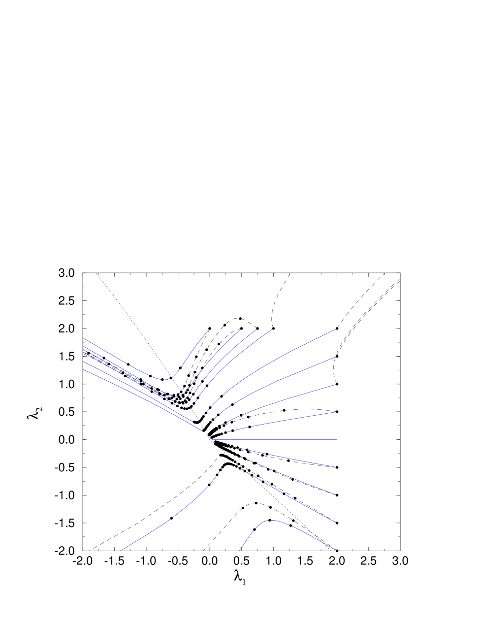
Figure 1:

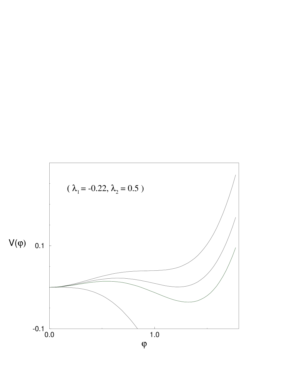
Figure 2:

Figure 3:

Figure 4:

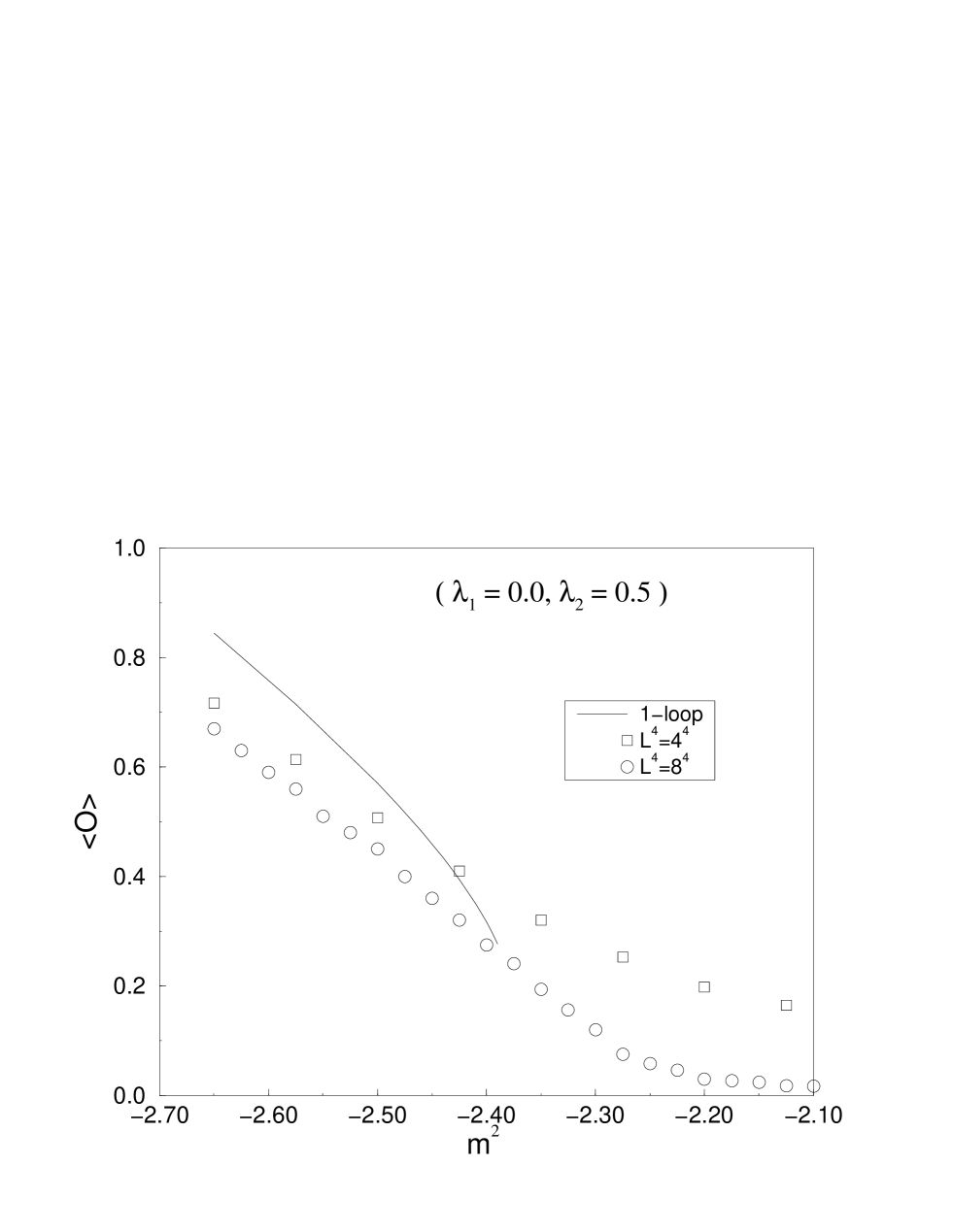
Figure 5:

Figure 6:

Figure 7:

Figure 8:

Figure 9:

Figure 10:

References

-
[1]
S. Dimopoulos and L. Susskind,
Nucl. Phys. B155 (1979) 237;
E. Eichten and K. D. Lane Phys. Lett. B90 (1980) 125. -
[2]
T. Appelquist, T. Takeuchi, M. Einhorn and L. C. R. Wijewardhana,
Phys. Lett. B220 (1989) 223;
T. Takeuchi, Phys. Rev. D40 (1989) 2697;
V. A. Miransky and K. Yamawaki, Mod. Phys. Lett. A4 (1989) 129. -
[3]
Y. Nambu, Enrico Fermi Institute Report, No. EFI 88-39 (unpublished);
V. A. Miransky and M. Tanabashi and K. Yamawaki, Phys. Lett. B221 (1989) 177; Mod. Phys. Lett. A4 (1989) 1043;
W. A. Bardeen, C.T. Hill and M. Lindner, Phys. Rev. D41 (1990) 1647. - [4] R.S. Chivukula, M. Golden and E. H. Simmons, Phys. Rev. Lett. 70 (1993) 1587.
- [5] R. S. Chivukula, A. G. Cohen and K. D. Lane, Nucl. Phys. B343 (1990) 554.
- [6] A. Hasenfratz, P. Hasenfratz, K. Jansen, J. Kuti and Y. Shen Nucl. Phys. B365 (1991) 79.
-
[7]
For a review see, for example, J. Smit,
Nucl. Phys. B (Proc. Suppl.) 17 (1990) 3;
J. Shigemitsu, Nucl. Phys. B (Proc. Suppl.) 17 (1990) 3. - [8] W. A. Bardeen, C. T. Hill and D.-U. Jungnickel Phys. Rev. D 49 (1994) 1437.
- [9] Y. Shen, Phys. Lett. 315B (1993) 146.
- [10] A.J. Paterson Nucl. Phys. 190B (1981) 188.
- [11] S. Coleman and E. Weinberg, Phys. Rev. D7 (1973) 1888.
- [12] H. Yamagishi Phys. Rev. 23 D (1981) 1880.
- [13] R.H. Pisarski and D.L. Stein, Phys. Rev. 23B (1981) 3549; J. Phys. 14 A (1981) 3341.
- [14] M. E. Machacek and M. T. Vaughn, Nucl. Phys. B236 (1984) 221; B249 (1985) 70.
- [15] J. Kuti, L. Lin and Y. Shen, Nucl. Phys. B (Proc. Suppl.) 4 (1988) 397.
-
[16]
U. M. Heller, M. Klomfass, H. Neuberger and P. Vranas,
Nucl. Phys. B405 (1993) 555;
M. Göckeler, H. A. Kastrup, T. Neuhaus and F. Zimmermann, Nucl. Phys. B404 (1993) 517. -
[17]
W. Bock, H.G. Evertz, J. Jersak, D.P. Landau, T. Neuhaus and J.L. Xu,
Phys. Rev. D41 (1990) 2573.
P. Arnold, S. Sharpe, L. G. Yaffe and Y. Zhang, hep-ph 9611201;
P. Arnold and Y. Zhang, hep-lat 9610032, hep-ph 9610448;
P. Arnold and L. G. Yaffe, hep-ph 9610447. - [18] D. Amit in, Field theory the Renormalization Group and critical phenomena, World Scientific 1984.
-
[19]
S. Duane, A.D. Kennedy, B.J. Pendleton and D. Roweth,
Phys. Lett. 195B (1985) 216;
A.L. Ferreira and R. Toral, Phys. Rev. 47E (1993) 3848.