June 1996 HU Berlin–EP–96/17
IFUP–TH 29/96
SWAT/96/108

$\mbox{}^{1}$ INFN in Pisa and Dipartimento di Fisica dell’Universitá di Pisa, Italy
$\mbox{}^{2}$ Humboldt-Universität zu Berlin, Institut für Physik, 10099 Berlin, Germany
$\mbox{}^{3}$ Department of Physics, University of Wales, Swansea, U.K.

We compare different conjugate gradient – like matrix inversion methods (CG, BiCGstab1 and BiCGstab2) employing for this purpose the compact lattice quantum electrodynamics (QED) with Wilson fermions. The main goals of this investigation are the CPU time efficiency of the methods as well as the influence of machine precision on the reliability of (physical) results especially close to the ’critical’ line $~{}\kappa_{c}(\beta)$.

1 Introduction

In many physical applications it is necessary to perform the inversion of some large $~{}N\times N~{}$ matrix $~{}{\cal M}$, i.e., to solve the equation

$${\cal M}\cdot X=\varphi~{},$$ (1)

where $~{}\varphi~{}$ is some known input–vector and $~{}X~{}$ the required solution. It becomes not an easy computational task to calculate the vector $~{}X~{}$ when, for example, $~{}N\mbox{}_{\textstyle\sim}^{\textstyle>}10^{4}~{}$ especially when $~{}{\cal M}~{}$ is not well–conditioned. The problem of efficiency and reliability of the inversion algorithm appears to be of crucial importance. The lattice approach to gauge theories (e.g., QED or QCD) which provides a powerful tool for the numerical study of quantum field theories in the nonperturbative regime is a typical example. In the case of the $~{}U(1)~{}$ gauge group and Wilson fermions (QED) the matrix to be inverted is [2]

$${\cal M}(U;\kappa) \equiv \hat{1}-\kappa\cdot Q(U),$$

$$Q_{xy}(U) = \sum_{\mu=1}^{4}\Bigl{[}\delta_{y,x+\hat{\mu}}\cdot({\hat{1}}-\gamma_{\mu})\cdot U_{x\mu}+\delta_{y,x-\hat{\mu}}\cdot({\hat{1}}+\gamma_{\mu})\cdot U_{x-\hat{\mu},\mu}^{\dagger}\Bigr{]}~{},$$ (2)

where $~{}x,y~{}$ denote the sites of a $~{}4d~{}$ lattice, $~{}{\hat{\mu}}~{}$ is the unit vector in the direction $~{}\mu~{}$, and $~{}\gamma_{\mu}$’s are $~{}4\times 4~{}$ Dirac’s matrices in euclidean space. The set of gauge field link variables $~{}\left\{U_{x\mu}\right\},~{}~{}U_{x\mu}\in U(1)~{}$ generated with the proper statistical weight defines the corresponding gauge field configuration, and the hopping parameter $~{}\kappa~{}$ is related to the bare mass of the fermion [2]. The dimension of the fermionic matrix is $~{}N\times N$ with $N=4\cdot N_{sites}$, and the typical number of sites in lattice calculations is $~{}N_{sites}\sim 8^{4}\div 20^{4}~{}$.

In our study we were especially interested in the physically most interesting – and technically most difficult – ’extreme’ case, when the minimal eigenvalue $~{}\lambda_{min}~{}$ of the fermionic matrix $~{}{\cal M}~{}$ tends to zero. In the case of Wilson’s fermionic matrix this limit is connected with the special choice of the hopping parameter $~{}\kappa\rightarrow\kappa_{c}(\beta)$, $~{}\beta~{}$ being the gauge coupling parameter, and is supposed to correspond to the chiral limit of the theory (see, e.g., [3]). By approaching the chiral limit within the confinement phase the most common matrix inversion methods like conjugate gradient (CG) or minimal residue (MR) become extremely inefficient or fail (for review see, e.g., [4]) according to the fact that the condition number of the fermionic matrix diverges.

Recently new very promising cg–like matrix inversion algorithms have been proposed : BiCGstab1 [5] and BiCGstab2 [6]. The successful application of BiCGstab1 to lattice gauge theory issues has been demonstrated in [7] for intermediate quark masses, i.e., for $~{}\kappa$’s sufficiently below $~{}\kappa_{c}(\beta)$. In this case the CPU time improvement factor was reported to be of about 2$\div$3 compared to CG. Similar improvement was reported also for the BiCGstab2 method [8, 9]. However, the problem of the efficiency and reliability of these methods in the $~{}\lambda_{min}\to 0~{}$ limit deserves further study. A delicate point to be studied is the possible breakdown because of the accumulation of roundoff errors. This accumulation becomes much more dangerous when approaching the chiral limit and/or when the precision of the used machine is not large, as in the case of APE/Quadrics. On this machine, the native single precision arithmetic can be improved using accurate summation methods [10] but which cannot fully compete with hardware supported double precision and require more computational power. Another interesting question which did not attract still sufficient attention is the the connection between the convergence of the residue vectors and the convergence of observables. As it will be shown, this connection can be rather nontrivial.

The above mentioned topics constitute the main goals of this work. In the second section we give a short description of the inversion methods under study and main notations. The third section is devoted to the reliability of the inversion methods, while in section four we present the CPU time improvement factors. The last section contains our conclusions.

2 Methods and observables

The structure of the fermionic matrix $~{}{\cal M}~{}$ in eq.(2) permits an optimization based on an even–odd decomposition [11, 12] :

$${\cal M}=\left(\begin{array}[]{cc}\hat{1}_{o}&\kappa\cdot Q_{oe}\\ \kappa\cdot Q_{eo}&\hat{1}_{e}\\ \end{array}\right),$$ (3)

where subscripts e and o stand for the even and odd subspace, correspondingly. Therefore, it is sufficient to invert, say, the matrix $~{}{\cal D}_{e}~{}$

$${\cal D}_{e}=\hat{1}_{e}-\kappa^{2}Q_{eo}Q_{oe}~{},$$ (4)

defined only on the even subspace in order to solve the problem (1) since the solution vector of the complementary subspace can be easily constructed from the solution $~{}X_{e}$. Throughout this work we refer to the even–odd preconditioned versions of the investigated algorithms.

We made a comparative study of the standard conjugate gradient method (CG), biconjugate gradient stabilized (BiCGstab1) and biconjugate gradient stabilized II (BiCGstab2). These methods approximate the true solution iteratively by generating a sequence $~{}X_{0},X_{1},\ldots,X_{k},\ldots$, where $~{}X_{0}~{}$ denotes the starting vector which can be chosen with different methods, for example in a random way. For completeness we give a short schematic description of these methods. To keep the notation simple we drop the subspace index in the algorithmic part of the formulas.

• CG. The equation to solve is ${\cal D}X_{e}=\varphi^{\prime\prime}_{e}={\cal D}_{e}^{\dagger}\varphi^{\prime}_{e}={\cal D}_{e}^{\dagger}\bigl{(}\varphi_{e}-\kappa Q_{eo}\varphi_{o}\bigr{)}$, with ${\cal D}={\cal D}_{e}^{\dagger}{\cal D}_{e}$.

  $P_{0}=R_{0}=\varphi^{\prime\prime}-{\cal D}X_{0}\\$ For  $k=0,\ldots~{}$:

  $$X_{k+1} = X_{k}+\omega_{k}P_{k}~{};\quad\omega_{k}=\bigl{(}R_{k},R_{k}\bigr{)}/\bigl{(}P_{k},{\cal D}P_{k}\bigr{)}$$

  $$R_{k+1} = R_{k}-\omega_{k}{\cal D}P_{k}$$

  $$P_{k+1} = R_{k+1}+\gamma_{k+1}P_{k}~{};\quad\gamma_{k+1}=\bigl{(}R_{k+1},R_{k+1}\bigr{)}/\bigl{(}R_{k},R_{k}\bigr{)}~{}.\qquad\qquad$$

  This method is simple in implementation and reliable, though it is not the fastest. In the version with double precision we use it as a reference point for the other two methods.

• BiCGstab1. The equation to solve is ${\cal D}X_{e}=\varphi^{\prime}_{e}$, with ${\cal D}={\cal D}_{e}$.

  $V_{0}=P_{0}=0\\ \alpha_{0}=\omega_{0}=\rho_{0}=1\\ R_{0}=\hat{R}_{0}=\varphi^{\prime}-{\cal D}X_{0}$
  
  For   $k=1,\ldots~{}$:

  $$\rho_{k} = \bigl{(}\hat{R_{0}},R_{k-1}\bigr{)}~{};\quad\beta_{k}=\bigl{(}\rho_{k}\alpha_{k-1}\bigr{)}\big{/}\bigl{(}\rho_{k-1}\omega_{k-1}\bigr{)}\qquad\qquad\qquad\qquad~{}~{}~{}$$

  $$P_{k} = R_{k-1}+\beta_{k}\bigl{(}P_{k-1}-\omega_{k-1}V_{k-1}\bigr{)}\qquad\qquad\qquad\qquad\qquad\qquad$$

  $$V_{k} = {\cal D}P_{k}~{};\quad\alpha_{k}=\rho_{k}\big{/}\bigl{(}\hat{R}_{0},V_{k}\bigr{)}$$

  $$S_{k} = R_{k-1}-\alpha_{k}V_{k}$$

  $$T_{k} = {\cal D}S_{k}~{};\quad\omega_{k}=\bigl{(}T_{k},S_{k}\bigr{)}\big{/}\bigl{(}T_{k},T_{k}\bigr{)}$$

  $$X_{k} = X_{k-1}+\omega_{k}S_{k}+\alpha_{k}P_{k}$$

  $$R_{k} = S_{k}-\omega_{k}T_{k}~{}.$$

• BiCGstab2. The equation to solve is ${\cal D}X_{e}=\varphi^{\prime}_{e}$, with ${\cal D}={\cal D}_{e}$.

  $R_{0}=\hat{R}_{0}=\varphi^{\prime}-{\cal D}X_{0}\\ \mbox{choose}~{}~{}Y_{0}~{}~{}\mbox{such that}~{}~{}\delta_{0}=\bigl{(}Y_{0},R_{0}\bigr{)}\not=0~{}~{}\mbox{and}~{}~{}\omega_{0}^{-1}=\bigl{(}Y_{0},{\cal D}\hat{R}_{0}\bigr{)}/\delta_{0}\not=0\\$ For $k=0,\ldots~{}:$

  $$V_{k+1} = U_{k}-\omega_{k}{\cal D}T_{k}~{},~{}~{}k\geq 1\qquad$$

  $$U_{k+1} = R_{k}-\omega_{k}{\cal D}\hat{R}_{k}$$

  $$\mbox{\text@underline{If}}~{}~{}k~{}~{}\mbox{even~{}~{}\text@underline{then}}~{}~{}m:=k/2$$

  $$\chi_{m} = \bigl{(}{\cal D}U_{k+1},U_{k+1}\bigr{)}\big{/}\bigl{(}{\cal D}U_{k+1},{\cal D}U_{k+1}\bigr{)}$$

  $$R_{k+1} = U_{k+1}-\chi_{m}{\cal D}U_{k+1}$$

  $$X_{k+1} = X_{k}+\omega_{k}\hat{R}_{k}+\chi_{m}U_{k+1}$$

  $$\delta_{k+1} = \bigl{(}Y_{0},R_{k+1}\bigr{)}~{};\quad\psi_{k+1}=-\bigl{(}\omega_{k}\delta_{k+1}\bigr{)}\big{/}\bigl{(}\chi_{m}\delta_{k}\bigr{)}$$

  $$\hat{R}_{k+1} = R_{k+1}-\psi_{k+1}(\hat{R}_{k}-\chi_{m}{\cal D}\hat{R}_{k})$$

  $$\mbox{\text@underline{else}}~{}~{}~{}m:=(k-1)/2$$

  $$B_{m+1} = [U_{k+1}-V_{k+1}|{\cal D}U_{k+1}]~{}~{}\mbox{(2 column matrix)}$$

  $$\left(\begin{array}[]{c}\xi_{m}\\ \eta_{m}\\ \end{array}\right) = -(B_{m+1}^{+}B_{m+1})^{-1}B_{m+1}^{+}V_{k+1}$$

  $$R_{k+1} = (1-\xi_{m})V_{k+1}+\xi_{m}U_{k+1}+\eta_{m}{\cal D}U_{k+1}$$

  $$X_{k+1} = (1-\xi_{m})(X_{k-1}+\omega_{k-1}\hat{R}_{k-1}+\omega_{k}T_{k})+\xi_{m}(X_{k}+\omega_{k}\hat{R}_{k})-\eta_{m}U_{k+1}$$

  $$\delta_{k+1} = \bigl{(}Y_{0},R_{k+1}\bigr{)}~{};\quad\psi_{k+1}=\bigl{(}\omega_{k}\delta_{k+1}\bigr{)}\big{/}\bigl{(}\eta_{m}\delta_{k}\bigr{)}$$

  $$\hat{R}_{k+1} = R_{k+1}-\psi_{k+1}\Bigl{(}(1-\xi_{m})T_{k}+\xi_{m}\hat{R}_{k}+\eta_{m}{\cal D}\hat{R}_{k}\Bigr{)}$$

  endif

  $$T_{k+1} = U_{k+1}-\psi_{k+1}\hat{R}_{k}~{};\quad{\cal D}T_{k+1}={\cal D}U_{k+1}-\psi_{k+1}{\cal D}\hat{R}_{k}$$

  $$\omega_{k+1} = \delta_{k+1}\big{/}\bigl{(}Y_{0},{\cal D}\hat{R}_{k+1}\bigr{)}~{}.$$

Compared to BiCGstab1 this algorithm has more complicated recurrences and requires more dot product operations.

The iterative procedure was stopped when $~{}||R_{k}||<\varepsilon~{}$. We used $~{}\varepsilon=10^{-5}~{}$ when implemented on an APE/Quadrics system (equivalent to the condition $||R_{k}||_{norm}\equiv||R_{k}||/||R_{0}||~{}\mbox{}_{\textstyle\sim}^{\textstyle<}~{}10^{-7}~{}$ on an $~{}8^{3}\times 16~{}$ lattice), and $~{}\varepsilon=5\cdot 10^{-8}~{}$ on double precision machines. A point to mention is that the matrix to be inverted in the case of CG is ${\cal D}={\cal D}_{e}^{\dagger}{\cal D}_{e}$ and hence differs from the BiCGstab1/2 cases where ${\cal D}={\cal D}_{e}$. The application of the same stopping criterion $~{}||R_{k}||<\varepsilon~{}$ to the different algorithms entails a systematic error, which we have found to be 0$\div$2%.

The algorithmic residue vectors $~{}R_{k}^{algo}=R_{k}~{}$ can differ substantially from the corresponding true residue vectors $~{}R_{k}^{true}=\varphi-{\cal D}X_{k}~{}$ due to roundoff errors. Apart from the norms of the two residue vectors ($||R^{true}_{k}||~{}$ and $||R^{algo}_{k}||$) we monitored also for every configuration the convergence of the pion norm $~{}\Pi~{}$, scalar condensate $~{}{\bar{\psi}}\psi~{}$ and pseudoscalar condensate $~{}{\bar{\psi}}\gamma_{5}\psi$ defined as :

$$\Pi = \frac{1}{4N_{sites}}\cdot\mbox{Tr}\Bigl{[}{\cal M}^{-1}\gamma_{5}{\cal M}^{-1}\gamma_{5}\Bigr{]}~{};$$ (6)

$${\bar{\psi}}\psi = \frac{1}{4N_{sites}}\cdot\mbox{Tr}\Bigl{[}{\cal M}^{-1}\Bigr{]}~{};\qquad{\bar{\psi}}\gamma_{5}\psi=\frac{1}{4N_{sites}}\cdot\mbox{Tr}\Bigl{[}\gamma_{5}{\cal M}^{-1}\Bigr{]}~{}.$$ (7)

It is useful to write down the spectral representation of these observables

$$\Pi = \frac{1}{4N_{sites}}\sum_{n}\frac{1}{\mu_{n}^{2}}~{};$$

$${\bar{\psi}}\psi = \frac{1}{4N_{sites}}\sum_{n}\frac{1}{\lambda_{n}}~{};\qquad{\bar{\psi}}\gamma_{5}\psi=\frac{1}{4N_{sites}}\sum_{n}\frac{1}{\mu_{n}}~{},$$ (8)

where $~{}\lambda_{n}~{}$ and $~{}\mu_{n}~{}$ denote the eigenvalues of $~{}{\cal M}~{}$ and $~{}{\cal M}\gamma_{5}$, respectively. Since $~{}\mu_{n}\to 0~{}$ when the corresponding $~{}\lambda_{n}\to 0$, it becomes clear why $~{}\Pi~{}$ is a very sensible observable near $~{}\kappa_{c}(\beta)$.

The conventional definition of the bare fermion mass $~{}m_{q}~{}$ is

$$m_{q}=\frac{1}{2}\cdot\Bigl{(}\frac{1}{\kappa}-\frac{1}{\kappa_{c}(\beta)}\Bigr{)}.$$ (9)

To monitor the influence of the accuracy we performed our calculations on a Cray–YMP and Siemens–Fujitsu (default 64bit, i.e., double precision), Convex–C3820–ES (single and double precision) and a QH2 – $~{}8\times 8\times 4~{}$ APE/Quadrics semitower. The native single precision of QH2 was improved by implementation of the Kahan summation method applied to global sums [10].

The lattice sizes we used have been $~{}16^{3}\times 32~{}$ and $~{}32^{3}\times 64~{}$ on the QH2, and $~{}8^{3}\times 16~{}$ and $~{}16^{3}\times 32~{}$ on the vector machines. The choice of the gauge coupling parameter $~{}\beta~{}$ was $~{}0~{}$ and $~{}0.8~{}$ in the confinement phase and $~{}1.1~{}$ in the Coulomb phase.

3 Reliability and precision effects

3.1 CG in single and double precision modes

One way to study the reliability of the inversion method is to monitor the inversion history of the two residues : $~{}R^{true}~{}$ and $~{}R^{algo}$. In the case of the double precision conjugate gradient method (CGDP) the norms of these two residues coincide with high accuracy down to very small values which ensures the reliability of the result. In Figure 1a we show an example of such a run at $~{}\beta=0.8~{}$ and $~{}\kappa=0.2170~{}$ on an $~{}8^{3}\times 16~{}$ lattice. The value of the hopping parameter $~{}\kappa~{}$ was chosen to be rather close to the critical value $~{}\kappa_{c}(\beta=0.8)\simeq 0.2171(1)$.

To our experience, CGDP never fails, although can become very slow. Therefore, we used the double precision conjugate gradient method as a reference point for the two ’stabilized’ methods and for CG in single precision mode (CGSP).

To single out the effect of machine accuracy, we applied the single precision and double precision CG to the same configurations providing the same startvectors and sourcevectors (see, e.g., Figure 1a).

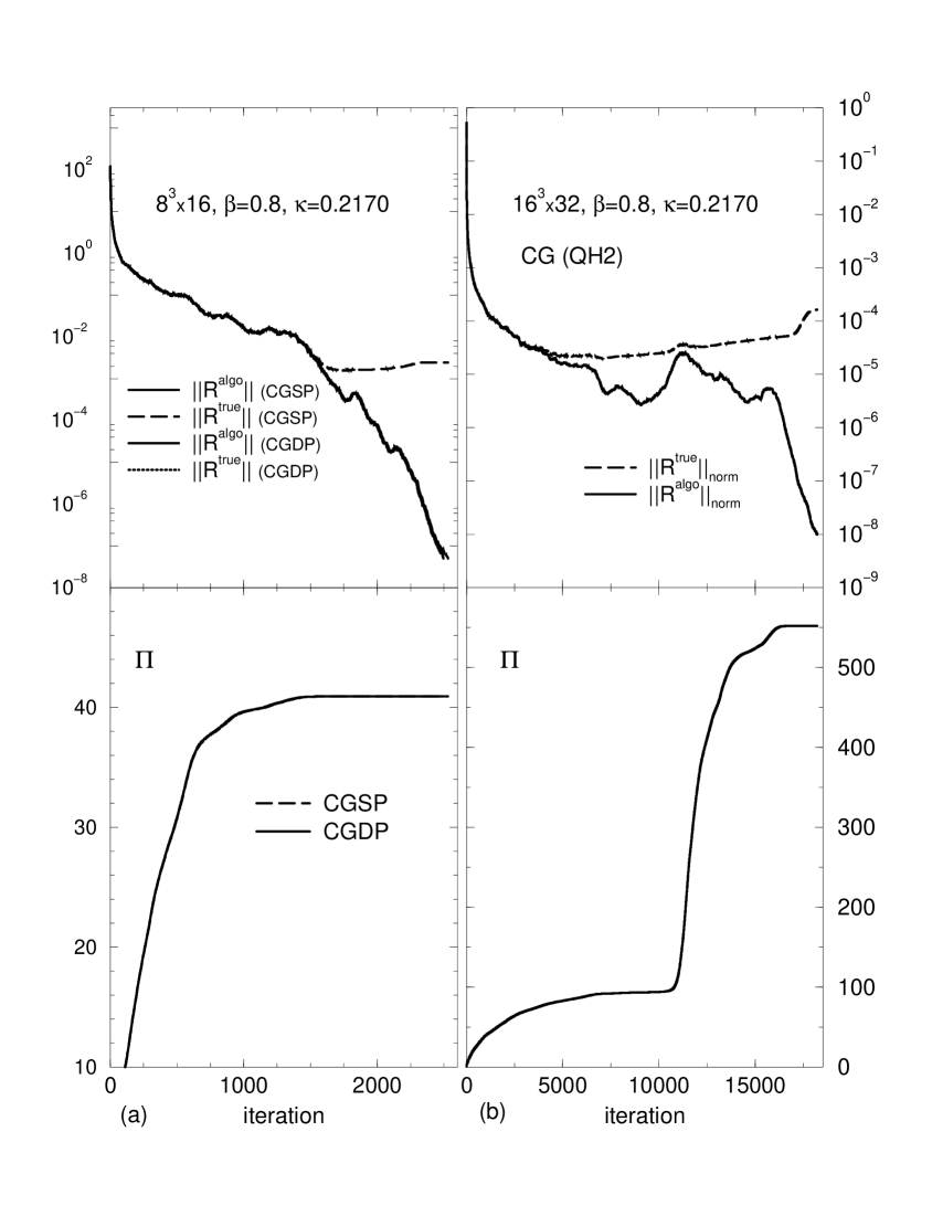
Figure 1: Convergence histories on single configurations on a vector machine (a) and QH2 (b). $||R_{k}||_{norm}=||R_{k}||/||R_{0}||$.

The single precision residue $~{}||R_{k}^{true}||~{}$ decouples from the other residues after $~{}\sim 1500~{}$ iterations due to lack of accuracy. However, the single precision algorithmic residue $~{}||R_{k}^{algo}||~{}$ coincides with both double precision residues. In this case the pion norm $~{}\Pi~{}$ practically does not depend on the machine accuracy. It reaches its plateau before $~{}||R_{k}^{true}||~{}$ has decoupled from the other residues.

Figure 2: The relative deviation $~{}\delta~{}$ as defined in eq.(10) at $~{}\kappa=0.25$ (a) and $~{}\kappa=0.2498$ (b).

In some cases, however, the decoupling of $~{}||R_{k}^{algo}||~{}$ and $~{}||R_{k}^{true}||~{}$ occurs before the observable (e.g., the pion norm) reaches its plateau. An example of such an inversion history on the QH2 (single precision) for $~{}\kappa=0.2170~{}$ is shown in Figure 1b. Despite the Kahan improved summation, $~{}||R^{true}_{k}||~{}$ starts even to increase long before the plateau in $~{}\Pi~{}$ is reached.

Attempting to determine the reliability of the single precision CG method in a more confidential way we compared the solutions for our fermionic observables given by CGSP to those of CGDP applied to a set of 200 gauge configurations for various values of $~{}\kappa~{}$ in the vicinity of $~{}\kappa_{c}~{}$ at $~{}\beta=0~{}$ on a $~{}8^{3}\times 16~{}$ lattice. On every configuration $~{}k~{}$ we checked the relative deviation

$$\delta(O^{k})=\frac{O^{k}_{DP}-O^{k}_{SP}}{O^{k}_{DP}}~{},$$ (10)

where $~{}O^{k}_{DP,SP}~{}$ denotes one of $~{}\bar{\psi}\psi,~{}\bar{\psi}\gamma_{5}\psi,~{}$ or $~{}\Pi~{}$ on the particular configuration obtained by CGDP or CGSP, respectively. Some results are given in Figure 2. In the case of $~{}\kappa=0.25~{}$ (see Figure 2a) the fermionic observables seem to be quite well reproduced by CGSP. The maximal relative deviations show up in $~{}\bar{\psi}\gamma_{5}\psi$, but remain under 3%. For the averages we obtain: $~{}\langle\delta(\bar{\psi}\psi)\rangle=-3\times 10^{-5}\pm 4\times 10^{-4},~{}\langle\delta(\bar{\psi}\gamma_{5}\psi)\rangle=2\times 10^{-4}\pm 3\times 10^{-3},~{}\langle\delta(\Pi)\rangle=-9\times 10^{-6}\pm 2\times 10^{-3}~{}.$ Therefore, the average ’IEEE–noise’ coming from the comparison of single to double precision data is well–consistent with zero within errorbars. However, at another – somewhat lower – value of $~{}\kappa~{}$ (Figure 2b) CGSP provided results which significantly differed from those of CGDP on some configurations and hence cannot be ignored. In particular, the maximal $~{}|\delta(\bar{\psi}\psi)|~{}$ is about $~{}\sim 20\%$. For the averages of $~{}\delta~{}$ we obtain $~{}\langle\delta(\bar{\psi}\psi)\rangle\sim-0.002\pm 0.02~{},~{}~{}\langle\delta(\bar{\psi}\gamma_{5}\psi)\rangle\sim-0.0004\pm 0.007~{}$ and $~{}\langle\delta(\Pi)\rangle\sim-0.0007\pm 0.09$, which, however, are still well consistent with zero. The maximal relative deviations observed on other values of $~{}\kappa~{}$ have been $~{}\sim 6\div 39\%$, demonstrating that CG in single precision mode is not a priori reliable in the ’critical’ region. Although the net effect of single precision on the CG method seemed to be small, i.e. the found averages of $~{}\delta~{}$’s are compatible with zero, it might happen that the averages of observables suffer from single precision, especially on sets of small statistics.

Therefore, the question about the reliability of the single precision (even Kahan improved) CG still remains open in the case of the confinement phase. More detailed study, especially on larger lattices, is necessary to draw a final conclusion here.

Fortunately, the situation is much more favorable in the Coulomb phase. The inversion procedure is comparatively fast both for $~{}\kappa~{}\mbox{}_{\textstyle\sim}^{\textstyle<}~{}\kappa_{c}~{}$ and $~{}\kappa>\kappa_{c}$. For all our observables we found very reasonable agreement between single precision and double precision calculations. As an example, we show in Figure 3 the average values of the pion norm $~{}\Pi~{}$ calculated with single (QH2) and double precision at $~{}\beta=1.1$. Since most of the DP data are obtained on a smaller lattice than the QH2 data there is a (rather weak) dependence of $~{}\langle\Pi\rangle~{}$ on the lattice size in the ’critical’ region around $~{}\kappa_{c}$. For the other values of $~{}\kappa~{}$ the agreement between CGDP and CG on the QH2 is very good. Since the vicinity of $~{}\kappa_{c}~{}$ is most interesting, we calculated four datapoints around $~{}\kappa_{c}~{}$ with CGDP on a $~{}16^{3}\times 32~{}$ lattice in order to compare them with the QH2 results from the same lattice size (see the inset of Figure 3). Obviously, the QH2 implementation of CG provides correct results at this $~{}\beta~{}$ value.

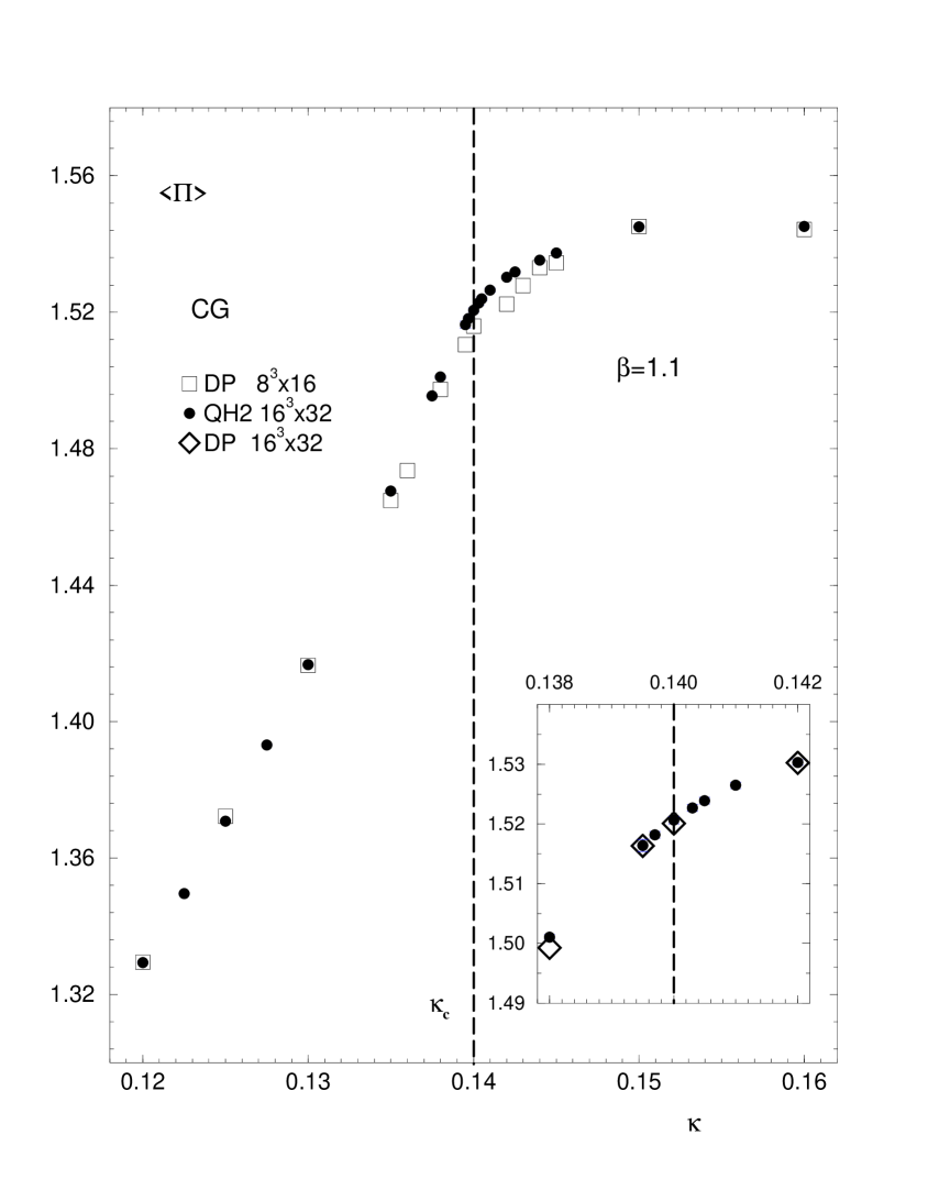
Figure 3: $~{}\langle\Pi\rangle~{}$ as a function of $~{}\kappa~{}$ at $~{}\beta=1.1$ obtained by CGSP (QH2) and CGDP. The vertical dashed line indicates the position of $~{}\kappa_{c}~{}$.

3.2 Double precision BiCG–stabilized methods

As in the previous subsection for CG we compared the ’stabilized’ methods by measuring fermionic observables on the same configurations. As long as the hopping parameter $~{}\kappa~{}$ was not too close to $~{}\kappa_{c}(\beta)~{}$ all three methods agreed with very high precision for all $~{}\beta$–values we used. However, at $~{}\kappa\to\kappa_{c}(\beta)~{}$ failures occurred even in the double precision mode, i.e. either the method did not converge at all or (as in the case of BiCGstab2) provided a solution deviating significantly from CGDP. As an example of non–convergence of BiCGstab1 we show in Figure 4 the first 4000 iterations of one inversion process at $~{}\beta=0~{}$ and $~{}\kappa=0.2496$. After $~{}20000~{}$ iterations we finally terminated the iterations. The norm of the residue vector $~{}||R^{algo}||$ ($||R^{true}||=||R^{algo}||$) did not decrease as expected and always remained larger than one. Both $~{}||R^{algo}||~{}$ and $~{}\Pi~{}$ stayed approximately constant when the number of iterations became larger than $~{}2500$. For comparison the dashed horizontal line shows the CGDP solution for the pion norm $~{}\Pi$. Restarting the procedure in some cases can help to resolve the problem. However, the effect of restarting seems to be rather sensible to the chosen frequency (see, e.g., [4], p.22).

Tables 1 to 3 show values of $~{}\beta~{}$ and $~{}\kappa~{}$ where failures of the different methods have been observed. The convergence of BiCGstab1 demonstrates an interesting $~{}\beta$–dependence. While in the extreme strong coupling limit $~{}\beta=0~{}$ it failed on some configurations in the limit $~{}\kappa\to\kappa_{c}(\beta)$, we did not observe failures at the larger $~{}\beta$–values in this limit. Failure rates of BiCGstab1 will be discussed in the next section.

As can be seen from these Tables BiCGstab2 appears to be less reliable when $~{}\kappa\sim\kappa_{c}$. Figure 5 illustrates the situation for different $~{}\kappa$–values at $~{}\beta=0.8$. For every $~{}\kappa$–value the pion norm $~{}\Pi~{}$ was calculated with the different methods on the same configuration. In the ’critical’ region (lower plot in Figure 5) BiCGstab1 matches CG with high precision, while BiCGstab2 fails. Near to $~{}\kappa_{c}(\beta)$ the number of failures of BiCGstab2 turned out to be very large. Therefore, we conclude that BiCGstab2 even in double precision mode is unsuitable for matrix inversion in the limit $~{}\lambda_{min}\to 0~{}$, i.e., $~{}\kappa\to\kappa_{c}(\beta)$. The comparative complexity of this algorithm turns out to be rather a disadvantage for the range of investigated values of $~{}\beta~{}$ and $~{}\kappa$. In particular, the calculation of the optimal coefficients $~{}\xi_{m}~{}$ and $~{}\eta_{m}~{}$ (see Section 2 and [6]) can be the source of numerical instability, since it involves operations like extra dot products, matrix inversion and rather complicated recurrences where roundoff errors can dramatically accumulate. This is quite likely what happens in the case $~{}\kappa\rightarrow\kappa_{c}(\beta)$.

We also performed runs at different $~{}\beta$’s and $~{}\kappa$’s in the ’critical’ region to compare the averages of different fermionic observables. Apart from the pion norm and fermionic condensate we calculated also for every configuration k the pseudoscalar correlator

$$\Gamma_{k}(\tau)\sim\sum_{{\vec{x}},{\vec{y}}}\left\{\mbox{Tr}\,\Bigl{(}{\cal M}^{-1}_{\,xy}\gamma_{5}{\cal M}^{-1}_{\,yx}\gamma_{5}\Bigr{)}-\mbox{Tr}\,\Bigl{(}{\cal M}^{-1}_{\,xx}\gamma_{5}\Bigr{)}\cdot\mbox{Tr}\,\Bigl{(}{\cal M}^{-1}_{\,yy}\gamma_{5}\Bigr{)}\right\}~{},\quad\tau=|x_{4}-y_{4}|$$

to determine the effective pion mass $~{}m_{\pi}(\tau)$. For $~{}\kappa$–values close to $~{}\kappa_{c}~{}$ we used an estimator defined in [18] to obtain a clear signal of $~{}m_{\pi}(\tau)$. In Figure 6 we show the $~{}\tau$–dependence of the effective ’pion’ mass $~{}m_{\pi}(\tau)~{}$ at $~{}\beta=0.8~{}$ and $~{}\kappa=0.2165$. Evidently, BiCGstab1 provides results well consistent with that obtained by CG.

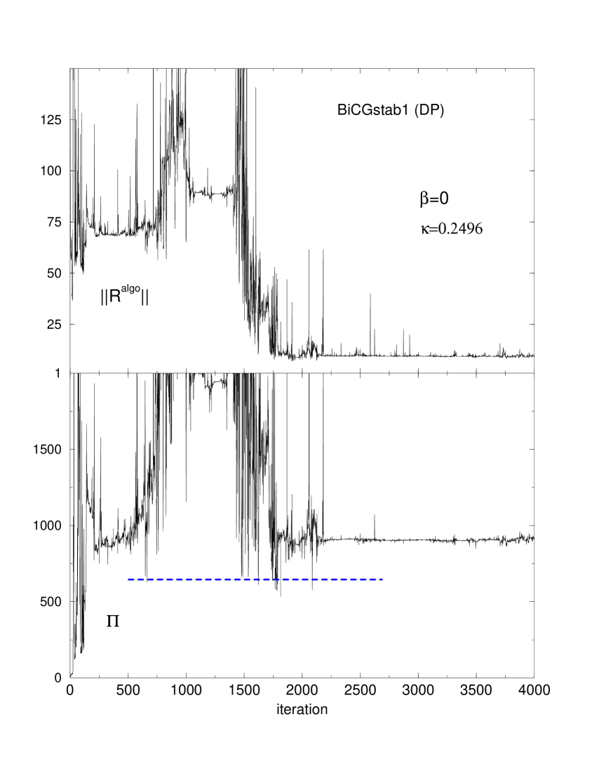
Figure 4: An inversion history of BiCGstab1 in double precision mode at $\beta=0$ and $\kappa=0.2496$. The dashed horizontal line marks the CGDP solution for $~{}\Pi~{}$. After $20000$ iterations the inversion process has been aborted.

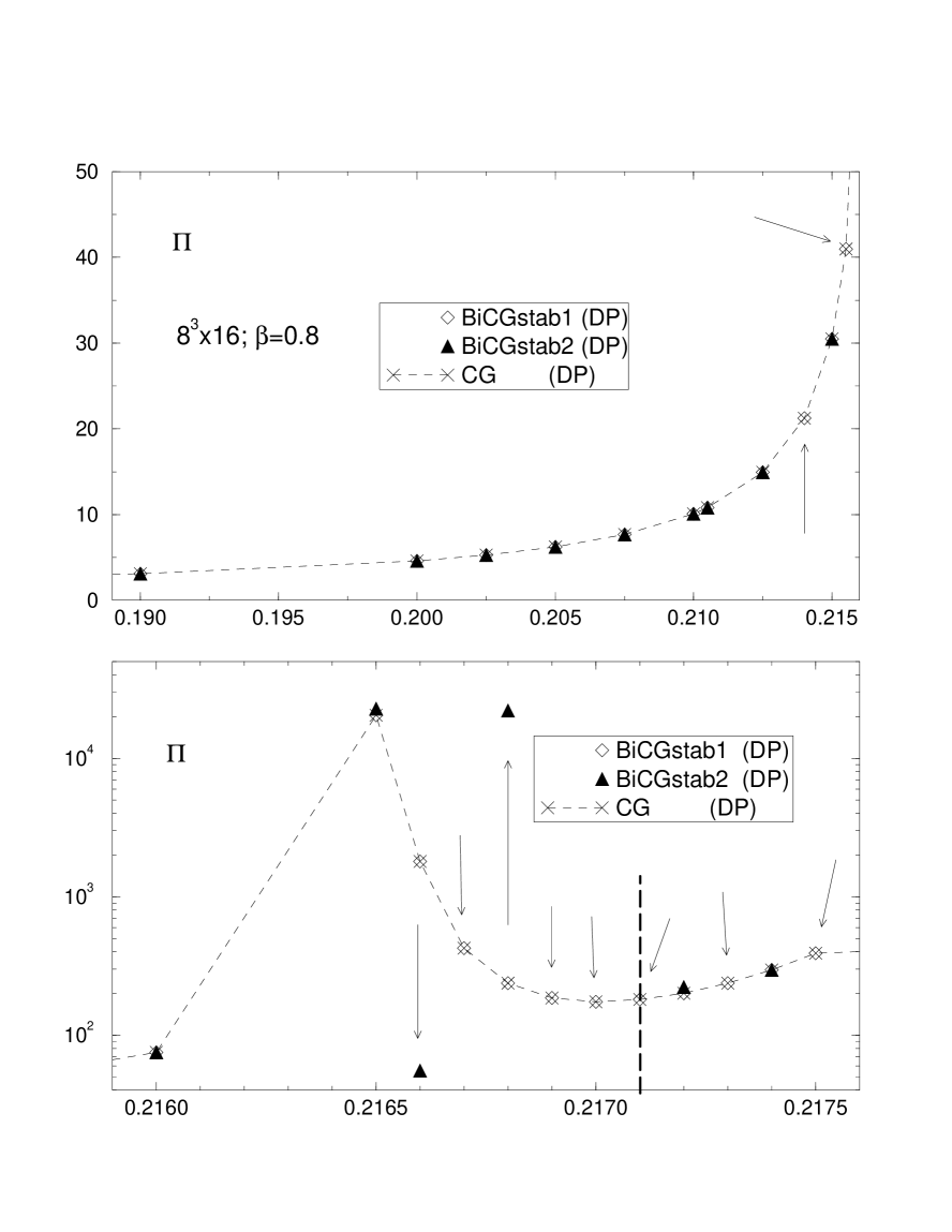
Figure 5: Pion norm $~{}\Pi~{}$ on individual configurations for CG, BiCGstab1 and BiCGstab2 in double precision mode. On the lower plot the $~{}\kappa~{}$ range is chosen to be in the vicinity of $~{}\kappa_{c}(\beta)~{}$ (vertical line). Arrows indicate where BiCGstab2 fails.

Figure 6: The $~{}\tau~{}$ dependence of the effective pseudoscalar mass $~{}m_{\pi}(\tau)$. The number of measurements is $~{}\sim 8000$.

3.3 Single precision BiCG–stabilized methods

This section is devoted to the comparison of the single precision and double precision BiCGstab methods. The main accent was made on the TAO–language realization of these algorithms on the APE/Quadrics machine (QH2). Since BiCGstab2 turned out to be unreliable (and in addition less efficient than BiCGstab1 – see the next section) for $~{}\kappa~{}$’s close to $~{}\kappa_{c}(\beta)~{}$ even in double precision we excluded this algorithm from further study on the QH2.

As an illustration, we show in Figure 7 the inversion history of the BiCGstab1–run performed on the QH2 at $~{}\beta=0.8$ and $~{}\kappa=0.214$. We have chosen here the configuration with the maximal number of iteration steps. The accumulation of roundoff errors entails the ramification of the two residues $||R^{algo}||$ and $||R^{true}||$. This is similar to the case of CG in single precision (compare to Figure 1). Note, that the Kahan summation which we used does not substantially increase the accuracy compared to unimproved single precision.

Figure 7: Normalized $~{}||R^{algo}||~{}$ and $~{}||R^{true}||~{}$ vs. inversion iterations for the BiCGstab1 method on the QH2 and the corresponding evolution of $~{}\Pi~{}$.

In Figure 8 we show the average of the pion norm $~{}\langle\Pi\rangle~{}$ as a function of $~{}\kappa~{}$ at $~{}\beta=0.8~{}$ on a $~{}16^{3}\times 32~{}$ lattice. For $~{}\kappa<0.214~{}$ we observe a very good agreement between BiCGstab1 and CG. We checked that these data are also well consistent with CGDP data, which are not shown in this $~{}\kappa$–region.

Figure 8: The average pion norm $~{}\langle\Pi\rangle~{}$ as a function of $~{}\kappa~{}$ obtained from CG and BiCGstab1 on the QH2. At $~{}\kappa=0.214;~{}0.215~{}$ we added also datapoints from CGDP. The position of $~{}\kappa_{c}(\beta)~{}$ is indicated by the vertical dashed line.

For $~{}\kappa>0.214~{}$ BiCGstab1 with single precision did not converge, in contrast to the double precision case at this value of $~{}\beta$. For all inversion methods, statistical averages and errorbars become ill-defined due to ’exceptional’ configurations close to $~{}\kappa_{c}(\beta)$ [18]. This effect is observable already at $~{}\kappa=0.214~{}$ and especially at $~{}\kappa=0.215~{}$.

Confinement phase $~{}\beta=0.8~{}$
		QH2		Double Precision
$\kappa$	$m_{q}$	CG	BiCGs1	CG	BiCGs1	BiCGs2
0.1900	0.3285	$\surd$	$\surd$	$\surd$	$\surd$	$\surd$
0.1950	0.2610	$\surd$	$\surd$	$\surd$	$\surd$	$\surd$
0.2000	0.1969	$\surd$	$\surd$	$\surd$	$\surd$	$\surd$
0.2100	0.0779	$\surd$	$\surd$	$\surd$	$\surd$	$\surd$
0.2105	0.0722	$\surd$	$\surd$	$\surd$	$\surd$	$\surd$
0.2114	0.0621	$\surd$	$\surd$	$\surd$	$\surd$	$\surd$
0.2118	0.0576	$\surd$	$\surd$	$\surd$	$\surd$	$\surd$
0.2125	0.0499	$\surd$	$\surd$	$\surd$	$\surd$	$\surd$
0.2140	0.0334	$\surd$	$\surd$	$\surd$	$\surd$	$\bigcirc$
0.2150	0.0225	?	$\bigcirc$	$\surd$	$\surd$	$\surd$
0.2160	0.0117	?	$\bigcirc$	$\surd$	$\surd$	$\bigcirc$
0.2170	0.0011	?	$\bigcirc$	$\surd$	$\surd$	$\bigcirc$
0.2171	0.0000			$\surd$	$\surd$	$\bigcirc$
0.2172				$\surd$	$\surd$	$\bigcirc$
0.2173				$\surd$	$\surd$	$\bigcirc$

Table 1: Reliability of inverters on $~{}16^{3}\times 32~{}$ (QH2) and $~{}8^{3}\times 16~{}$ lattices (double precision machine). Symbol $~{}\surd~{}$ denotes correct fermionic observables; $~{}\bigcirc~{}$ indicates a failure of the method. A question mark means that no conclusion could be drawn. $\kappa_{c}(\beta)$ is given by boldface.

Tables 1 to 3 summarize our results concerning the reliability of the inverter methods on the QH2 and on the double precision machines in the confinement and Coulomb phases. In the confinement phase single precision BiCGstab1 and BiCGstab2 were observed to fail at smaller values of $~{}\kappa~{}$ compared to the runs with double precision arithmetic, and therefore are unsuitable to explore the ’critical’ region. On the other hand, in the Coulomb phase BiCGstab1 on the QH2 proved to work even for $~{}\kappa=\kappa_{c}(\beta)$.

Confinement phase $~{}\beta=0~{}$
		Double Precision
$\kappa$	$m_{q}$	CG	BiCGs1	BiCGs2
0.2425	0.0619	$\surd$	$\surd$	$\surd$
0.2450	0.0408	$\surd$	$\surd$	$\surd$
0.2475	0.0202	$\surd$	$\surd$	$\surd$
0.2480	0.0161	$\surd$	$\surd$	$\surd$
0.2482	0.0145	$\surd$	$\surd$	$\surd$
0.2484	0.0129	$\surd$	$\surd$	$\surd$
0.2486	0.0113	$\surd$	$\surd$	$\surd$
0.2488	0.0096	$\surd$	$\surd$	$\surd$
0.2490	0.0080	$\surd$	$\surd$	$\bigcirc$
0.2492	0.0064	$\surd$	$\surd$	$\bigcirc$
0.2494	0.0048	$\surd$	$\bigcirc$	$\bigcirc$
0.2496	0.0032	$\surd$	$\bigcirc$	$\bigcirc$
0.2498	0.0016	$\surd$	$\bigcirc$	$\bigcirc$
0.2499	0.0008	$\surd$	$\bigcirc$	$\bigcirc$
0.2500	0.0000	$\surd$	$\bigcirc$

Table 2: Same as Table 1 but at $~{}\beta=0$.

Coulomb phase $~{}\beta=1.1~{}$
		QH2		Double Precision
$\kappa$	$m_{q}$	CG	BiCGs1	CG	BiCGs1	BiCGs2
0.13500	0.1323	$\surd$	$\surd$	$\surd$	$\surd$
0.13600	0.1050		$\surd$	$\surd$	$\surd$	$\surd$
0.13700	0.0782	$\surd$	$\surd$	$\surd$	$\surd$	$\surd$
0.13800	0.0518	$\surd$	$\surd$	$\surd$	$\surd$	$\surd$
0.13900	0.0257	$\surd$	$\surd$	$\surd$	$\surd$	$\surd$
0.13950	0.0128	$\surd$	$\surd$	$\surd$	$\surd$	$\bigcirc$
0.14000	0.0000	$\surd$	$\surd$	$\surd$	$\surd$	$\bigcirc$
0.14200		$\surd$	$\bigcirc$	$\surd$	$\surd$	$\bigcirc$
0.14400		$\surd$	$\bigcirc$	$\surd$	$\surd$	$\bigcirc$

Table 3: Same as Tables 1, 2 but in the Coulomb phase at $~{}\beta=1.1$.

To quantify the results of Tables 1, 2 we show in Figure 9 the failure rates of the single and double precision BiCGstab1 implementations in dependence on $~{}m_{q}$ obtained from 210 gauge configurations. We allowed the fermionic observables to deviate by a certain cutoff from the corresponding CGDP result on each configuration. The failure rates turned out to be almost insensitive to the special choice of the cutoff in both, single and double precision cases, when it was varied from $0.5\%$ to $40\%$. The results confirm, that the failure rate is drastically increased when single precision is used. It suggests also, that the double precision version of BiCGstab1 may be applied very close to $~{}\kappa_{c}~{}$ in the confinement phase. For instance, at $~{}\beta=0.8~{}$ the failure rate of the double precision BiCGstab1 has been found to be zero for all investigated values of $~{}\kappa$.

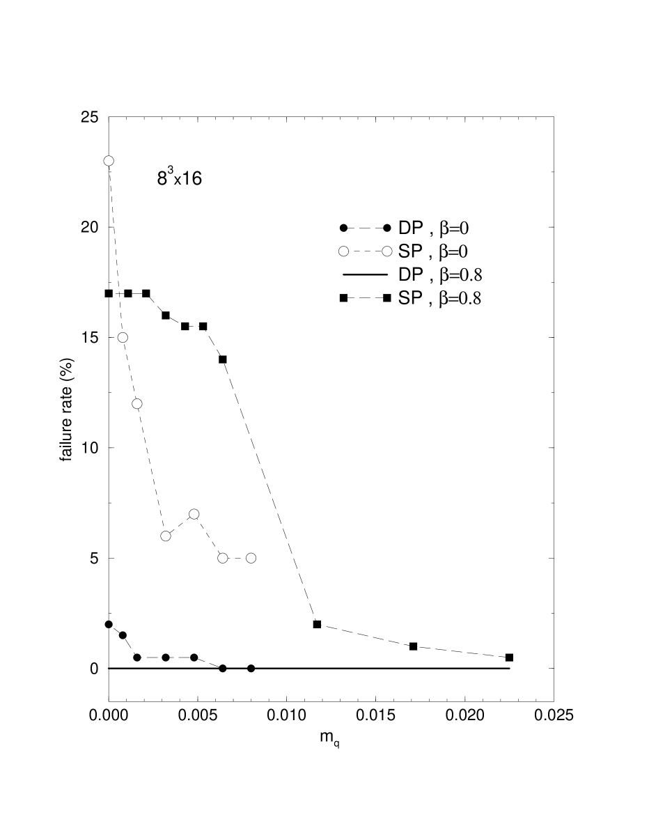
Figure 9: The failure rate (in $\%$) of BiCGstab1 for $~{}\beta=0~{}$ and $~{}\beta=0.8~{}$ in double and single precision modes. $m_{q}~{}$ is defined in eq.(9).

4 Efficiency

In the confinement phase the double precision BiCGstab1 demonstrates a pronounced superiority over CG and BiCGstab2 up to values of $~{}\kappa~{}$ rather close to $~{}\kappa_{c}(\beta)$. As an example, we show in Figure 10 the inversion history for CG and BiCGstab1 at $~{}\beta=0.8$ and $~{}\kappa=0.2170$ ($\kappa_{c}=0.2171(1)$) on an $~{}8^{3}\times 16~{}$ lattice in double precision mode. Both methods were applied to the same configuration. The data points for $~{}||R^{algo}||~{}$ and $~{}||R^{true}||~{}$ are on top of each other for both methods. The pion norm $~{}\Pi~{}$ reaches a plateau before the stopping criterion is fulfilled. As far as CG and BiCGstab1 require the same number of matrix multiplications per iteration their CPU time requirement per iteration is about the same. Viewed in this context, the small number of BiCGstab1 iterations compared to CG is impressive.

To quantify this point we compared the average CPU–times $~{}t_{cpu}~{}$ per inversion between the different methods. In the case of BiCGstab2 we compared $~{}t_{cpu}~{}$ for 10 configurations to the CPU–time required by BiCGstab1 on the same set of configurations including the same initial conditions. It turned out, that in the confinement phase at $~{}\beta=0.8~{}$ BiCGstab2 is by a factor $~{}\sim 0.6\div 0.9~{}$ less efficient than BiCGstab1, depending on the choice of $~{}\kappa$. In Figure 11 we display the comparative efficiency, i.e. the ratios $~{}t_{cpu}^{CG}\big{/}t_{cpu}^{BiCGstab1}~{}$ and $~{}t_{cpu}^{CG}\big{/}t_{cpu}^{BiCGstab2}~{}$ at $~{}\beta=0.8$ in dependence on $~{}\kappa$. The number of measurements for BiCGstab1 on the double precision machine has been 200, while on the QH2 it ranged from $\sim 80\div 800$.

BiCGstab1 yields a considerable gain in CPU time by a factor of $~{}\sim 3\div 5~{}$ on the QH2. This factor is supported by the double precision data and is comparable with findings from quenched QCD tests [7]. Note, that the comparative efficiency is rather stable with respect to the lattice size, since Figure 11 displays data from $~{}8^{3}\times 16~{}$ and $~{}16^{3}\times 32~{}$ lattices. In the case of $~{}\beta=0~{}$ the same picture holds qualitatively, however the maximal CPU time improvement factor was around 9 on double precision vector machines.

As mentioned, BiCGstab2, if reliable, was always less efficient than BiCGstab1 but a factor of $~{}\sim 2\div 3~{}$ better than CG.

Things change dramatically in the Coulomb phase (see Figure 12). The comparative efficiency of BiCGstab1 displays a sudden drop around $~{}\kappa_{c}$, the trend for BiCGstab2 is the same. Sufficiently below $~{}\kappa_{c}~{}$ the maximal factor of CPU time improvement is below 2 and goes to zero for $~{}\kappa\rightarrow\kappa_{c}(\beta)~{}$. BiCGstab2 has always found to be less efficient than BiCGstab1.

Presumably, the completely different distributions of eigenvalues of the fermionic matrix in the confinement and Coulomb phases cause this significantly different behavior of the inversion algorithms.

Figure 10: Convergence history for the double precision CG and BiCGstab1 at $\beta=0.8$ and $\kappa=0.2170$.

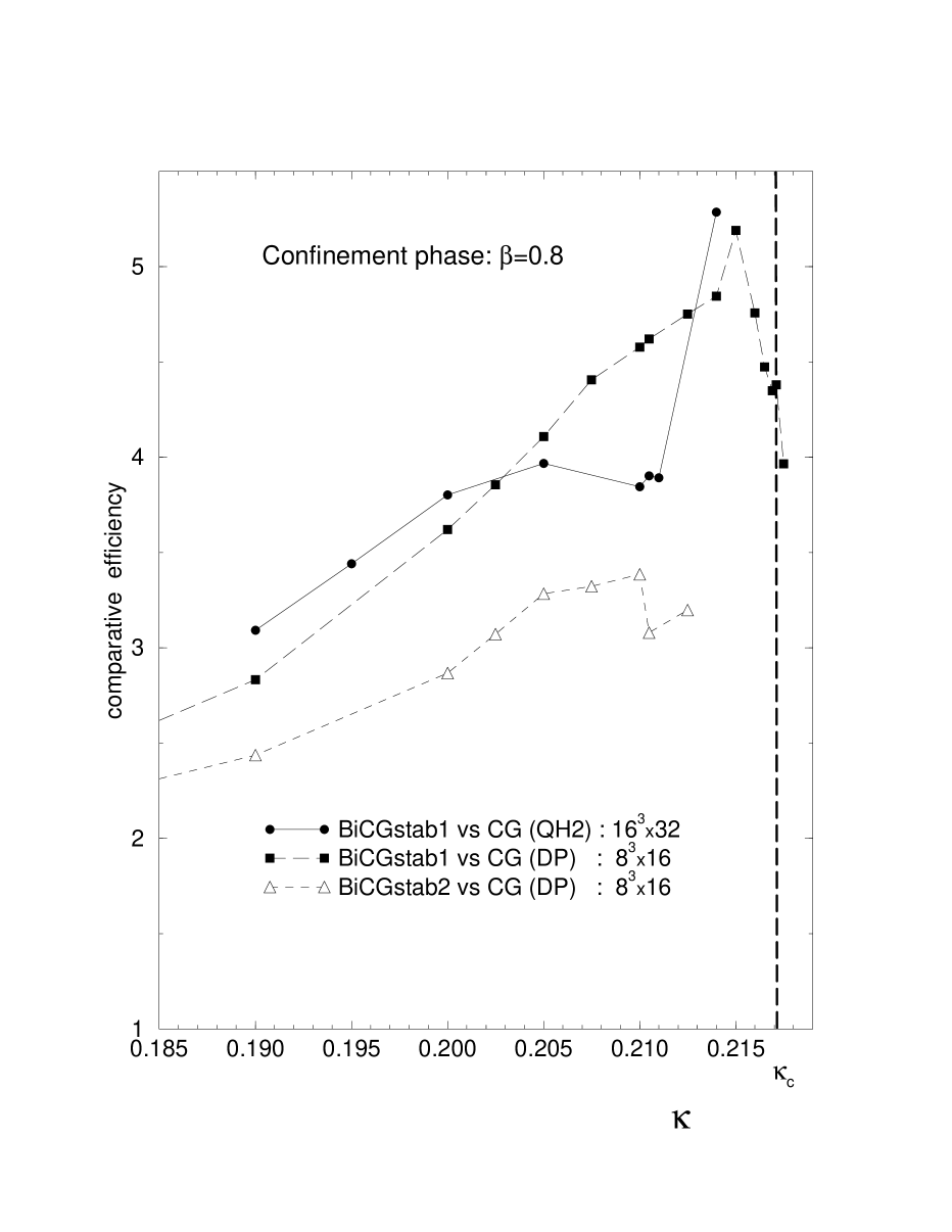
Figure 11: Comparative efficiency of BiCGstab1 and BiCGstab2 for different $\kappa$’s in the confinement phase at $\beta=0.8$. The vertical line indicates the position of $~{}\kappa_{c}$.

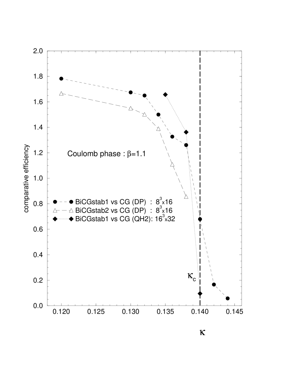
Figure 12: Same as Figure 11 but in the Coulomb phase at $\beta=1.1$.

5 Summary and conclusions

To summarize, we studied the reliability and comparative efficiency of the three matrix inversion methods : CG, BiCGstab1 and BiCGstab2. For this study we employed the $~{}U(1)~{}$ lattice gauge theory with Wilson fermions, the inverted matrix being an even-odd decomposed version of the Wilson fermionic matrix $~{}{\cal M}~{}$ (or $~{}{\cal M}^{\dagger}{\cal M}$). The main accent in our study was made on the ’critical’ case $\kappa\sim\kappa_{c}(\beta)$. The runs have been performed in double precision implementation (Cray, Convex, Siemens–Fujitsu) and in single precision implementation (Convex and especially QH2).

Our main conclusions are as follows.

• The standard CG with double precision appears to be the most reliable method, though not the fastest one. No failures were observed even at $~{}\kappa~{}\mbox{}_{\textstyle\sim}^{\textstyle>}~{}\kappa_{c}(\beta)$.

  The CG with single precision in the Coulomb phase, i.e., $\beta>\beta_{0}\simeq 1.01~{}$, is very reliable and reproduces the double precision results with reasonable accuracy even at $~{}\kappa=\kappa_{c}(\beta)$.

  In the confinement phase ($\beta<\beta_{0}$), however, the question of the reliabily of the CGSP in the $~{}\kappa\to\kappa_{c}(\beta)~{}$ limit still remains open.

• The reliability of the double precision BiCGstab1 is rather high when $~{}\kappa\sim\kappa_{c}(\beta)$. The failure rate is zero at $~{}\beta=0.8~{}$, and about 2% in the extreme case $~{}\beta=0$. Given some precautions for a fatal case, e.g. restarting or switching to another inverter, it can be used to study the limit $~{}\kappa\rightarrow\kappa_{c}(\beta)$.

  In the case of single precision in the confinement phase the reliability of the BiCGstab1 drastically drops in the $~{}\kappa\to\kappa_{c}(\beta)~{}$ limit.

• In the confinement phase in the $~{}\kappa$–region, where a comparison was possible, BiCGstab1 turned out to be the most efficient algorithm. The gain in CPU time was a factor of $~{}\sim 2.5\div 5~{}$ as compared to CG at $~{}\beta=0.8$, and up to a factor of $~{}\sim 9$ in the extreme strong coupling regime $~{}\beta=0$.

  This does not hold for the Coulomb phase, where BiCGstab1 (as well as BiCGstab2) exhibits a sudden drop in efficiency around $~{}\kappa_{c}(\beta)~{}$ and CG becomes the fastest method.

• BiCGstab2 even with double precision shows rather low reliability in the ’critical’ region $~{}\kappa\sim\kappa_{c}$. This fact practically excludes this method from the study of the chiral limit of the theory.

  In the parameter range, where BiCGstab2 worked, it was always less efficient than BiCGstab1 (by a factor $~{}\sim 0.6\div 0.9$).

The completely different behavior of the comparative efficiency found in the confinement and Coulomb phases suggests, that the optimal choice of the inversion algorithm is dictated by the typical distribution of eigenvalues in the particular phase. Further investigation is needed to work out this point.

We expect that most of the conclusions drawn in this paper can be applied also to lattice QCD.

Acknowledgements

A.H. and V.K.M acknowledge support by the Deutsche Forschungsgemeinschaft with research grant Mu 932/1-4. The calculations were performed in DESY–IFH Zeuthen, Konrad–Zuse–Zentrum Berlin, RRZN Hannover and RZ at Humboldt University Berlin. A.H., V.K.M. and M.M.-P. are grateful to Fr. Subklev from RZ for support.

References

- [1]
- [2] K. Wilson, Phys. Rev. D10 (1974) 2445; in New phenomena in subnuclear physics, ed. A. Zichichi (Plenum, New York, 1977).
- [3] A. Hoferichter, V.K. Mitrjushkin, M. Müller–Preussker, Th. Neuhaus and H. Stüben, Nucl. Phys. B434 (1995) 358.
- [4] R. Barret et al., Templates for the Solution of Linear Systems : Building Blocks for Iterative Methods SIAM, Philadelphia (1994).
- [5] H.A. van der Vorst, SIAM J. Sci. Comp. 13 (1992) 631.
- [6] M.H. Gutknecht, SIAM J. Sci. Comput. 14 (1993) 1020.
- [7] A. Frommer, V. Hannemann, B. Nöckel, Th. Lippert and K. Schilling, Int.J.Mod.Phys.C 5, No.6 (1994) 1073.
- [8] A. Borici and Ph. De Forcrand, IPS Research Report 94–03 (1994).
- [9] Ph. De Forcrand, IPS 95-24 (1995).
-
[10]
M. Lüscher and H. Simma,
Accurate Summation Methods for the APE-100 Parallel Computer, available at http://www.ifh.de/computing/parallel/ape/document.html. - [11] Th.A. DeGrand, Comput. Phys. Comm. 52 (1988) 161.
- [12] Th.A. DeGrand and P. Rossi, Comput. Phys. Comm. 60 (1990) 211.
- [13] N. Kawamoto and J. Smit, Nucl. Phys. B192 (1981) 100.
- [14] M.R. Hestenes and E. Stiefel, Journal of Research of the NBS 49 (1952) 409.
- [15] M. Engeli et al., Mitteilungen aus dem Institut für angewandte Mathematik (Birkhäuser Verlag, Berlin, 1959), Vol. 8, p. 24.
- [16] Ph. De Forcrand, A. König, K.-H. Mütter, K. Schilling and R. Sommer, in: Proc. Intern. Symp. on Lattice gauge theory (Brookhaven, 1986), (Plenum, New York, 1987).
- [17] Ph. De Forcrand, R. Gupta, S. Güsken, K.-H. Mütter, A. Patel, K. Schilling and R. Sommer, Phys. Lett. 200B (1988) 143.
- [18] A. Hoferichter, V.K. Mitrjushkin and M. Müller–Preussker, DESY 95–141 (1995).