Abstract

We use lattice sum rules for the static quark potential to determine the beta-function for symmetric and asymmetric lattices non-perturbatively. We also study the colour field distributions in excited gluonic states.

1 Introduction

In a lattice calculation, the observables are extracted as dimensionless ratios involving the lattice spacing $a$. It is important to obtain results for a range of $\beta$ (the bare lattice coupling coefficient given for $SU(N)$ by $2N/g^{2}$) in order to explore the approach to the continuum limit $a\to 0$. The region of small lattice corrections is reached when the lattice spacing $a$ obtained from different observables has a common $\beta$-dependence. Usually this has been explored by simulating at two different values of $\beta$ and matching the results. Another route to this information is from the lattice sum rule approach which allows [1, 2] a derivative of a lattice observable with respect to $\beta$ to be evaluated at a fixed $\beta$-value by summing plaquette contributions over all space. Expressing this in terms of a lattice spacing $a$ determined from that observable, the $\beta$-function $b=d\beta/d\ln a$ can then be extracted [3, 4]. Moreover, a generalisation to a lattice with different spacings $a_{i}$ in the four directions coming from a generalised Wilson action of the form $\beta_{ij}\Box_{ij}$ gives access [5] to derivatives with respect to these coefficients $\beta_{ij}$ by summing plaquettes in the $ij$ plane. It is thus possible to evaluate generalised $\beta$-functions

$${\partial\beta_{ij}\over\partial\ln a_{k}}=S\ \hbox{if}\ k=i\ \hbox{or}\ j\ \ \hbox{and}\ \ {\partial\beta_{ij}\over\partial\ln a_{k}}=U\ \hbox{if}\ k\neq i\ \hbox{or}\ j$$ (1)

by working on a symmetric lattice ($a_{i}=a$) at a fixed $\beta$ value.

For future comparison, the perturbative series for these quantities in terms of the bare lattice coupling $\alpha=g^{2}/4\pi=1/\pi\beta$ for $SU(2)$ colour fields are [6]

$$b=2(S+U)=-0.3715(1+0.49\alpha+\dots)\ \ \ \ \ \ \ U-S=2\beta f=2\beta(1-1.13\alpha+\dots)\ .$$ (2)

Here we use lattice sum rule techniques to calculate both $b$ and $f$ non-perturbatively.

We shall apply this sum rule technique to the potential between a static quark and antiquark at separation $R$. As well as a sum rule study to obtain the generalised $\beta$-functions from the ground state potential, we also explore excited gluonic potentials – both to determine the generalised $\beta$-functions and to compare with excited string models of the spatial distribution of the colour fields responsible for the gluonic excitation.

2 Sum rules for potentials

We consider the static quark potential for separation $R$ which is defined as $V(R)$ in lattice units. Then the colour fields associated with this pair of static quarks can be measured using plaquettes of appropriate orientation. Sum rules have been derived to relate the sum over all spatial positions of these colour fields to $V(R)$ and its derivative [5]:

$$V+R{\partial V\over\partial R}=b\sum({\cal E}_{L}+2{\cal E}_{T}+2{\cal B}_{T}+{\cal B}_{L})$$ (3)

$$V+R{\partial V\over\partial R}=-4\beta f\sum({\cal E}_{L}-{\cal B}_{L})$$ (4)

$$V-R{\partial V\over\partial R}=-4\beta f\sum({\cal E}_{T}-{\cal B}_{T})\ .$$ (5)

Here $L$ refers to longitudinal and $T$ to transverse with respect to the interquark separation axis. The notation is that ${\cal E}$ and ${\cal B}$ refer to the difference of the expectation values of the plaquette in the appropriate orientation in the presence of the static quarks and in the vacuum: ${\cal E}_{i}=\langle R|\Box_{i0}|R\rangle-\langle 0|\Box_{i0}|0\rangle$, etc., with $\Box={1\over 2}{\rm Tr}(1-U_{\Box})$. Thus they have the interpretation of gauge invariant averages of the fluctuation of squared strengths of the colour electric (${\cal E}$) and magnetic (${\cal B}$) fields. Since they are a difference between the value in the presence of the (generalised) Wilson loop representing the static quarks and the vacuum value, either sign is possible.

Because the combination ${\cal E}\pm{\cal B}$ corresponds to action/energy, we refer to these sum rules as ‘action’, ‘longitudinal energy’ and ‘transverse energy’ respectively.

The sum rules are derived [5] for torelons where there is no self energy associated with the static quarks. For the more practical case of the interquark potential between static sources, a self energy term must be included in each of the sum rules. This self energy will be independent of the inter-quark separation $R$ and hence can be removed exactly by considering differences of the sum rules for two different $R$-values.

The remaining obstacle to an evaluation of the sum rules is the presence of the derivative $dV/dR$. This arises in the sum rule derivation from re-expressing the derivative $dV(R)/d\beta$ at fixed number of lattice spacings $R$. In the limit of small lattice spacing $a$ and large number of lattice spacings $R$, this derivative can be accurately expressed in terms of $dV(R)/dR$ at fixed $\beta$. For small $R$, however, there may be substantial systematic error from relating the $\beta$-dependence at fixed $R$ to the $R$-dependence at fixed $\beta$. Thus we prefer to retain accuracy by eliminating $dV/dR$ from the sum rules. This leads to the relations which can be used to obtain $f$ and $b$:

$$V(R_{1})-V(R_{2})=-2\beta f\sum({\cal E}_{L}-{\cal B}_{L}+{\cal E}_{T}-{\cal B}_{T})_{R_{1}}-\sum({\cal E}_{L}-{\cal B}_{L}+{\cal E}_{T}-{\cal B}_{T})_{R_{2}}$$ (6)

$$b={2(V(R_{1})-V(R_{2}))\left(1+{\sum({\cal E}_{T}-{\cal B}_{T})_{R_{1}}-\sum({\cal E}_{T}-{\cal B}_{T})_{R_{2}}\over\sum({\cal E}_{L}-{\cal B}_{L})_{R_{1}}-\sum({\cal E}_{L}-{\cal B}_{L})_{R_{2}}}\right)^{-1}\over\sum({\cal E}_{L}+2{\cal E}_{T}+2{\cal B}_{T}+{\cal B}_{L})_{R_{1}}-\sum({\cal E}_{L}+2{\cal E}_{T}+2{\cal B}_{T}+{\cal B}_{L})_{R_{2}}}\ .$$ (7)

As well as using these sum rules for different values of $R$ to eliminate the self energy terms, it is also possible to use the difference between excited states and ground states. The derivation of the sum rules can be extended to the case of an excited state and the expressions are the same as those given in Eqs. (3), (4) and (5). The self energy is associated with the static quarks themselves and is also the same for excited states and ground states and so cancels fully for differences of energies between excited and ground states. In practice we use the E_u representation of D_4h to provide the most accessible excited state on a lattice. For more details on these excited potentials see ref [7, 8].

3 Lattice evaluation

We use a $16^{3}\times 32$ lattice at $\beta=2.4$ for this preliminary study with the $SU(2)$ gauge group. For many purposes $SU(2)$ colour provides an excellent test bed for QCD studies. In this work the scale as set by the string tension corresponds to a lattice spacing $a=0.6$ GeV^-1. Generalised Wilson loops of size $R\times T$ are evaluated with the spatial paths of length $R$ at $t=0$ and $T$ being constructed [9] from fuzzed links (using 2 and 13 recursive iterations of the projected sum of 4 $\times$ straight link $+$ 4 U-bends). We study the plaquette signal for all plaquette orientations at time slices $t=T/2$. The correlation of this plaquette sum with the Wilson loop then gives the required squared fluctuation of the colour field.

For the sum rule study, we need the sum of plaquettes over all space in principle. On the lattice, we sum the plaquettes over all transverse space (a $16\times 16$ plane) for each $r_{L}$. The sum over $r_{L}$ is then approximated by selecting the region within $\pm 2$ lattice units of the Wilson loop (ie from $r_{L}=-2$ to $R+2$). We checked that this approximation did not introduce any significant error since the missing $r_{L}$ region contributes noise and no signal to the correlation. The data sample used comes from a comprehensive study of 60 blocks of 125 measurements separated by 4 update sweeps (3 over-relaxation plus one heatbath). Error estimates use a full bootstrap analysis of these blocks.

The fuzzed link operator to create a static quark and antiquark at separation $R$ with colour field in a state of a given symmetry will have an expansion in terms of the eigenstates of the transfer matrix

$$|R\rangle=c_{0}|V_{0}\rangle+c_{1}|V_{1}\rangle+\dots$$ (8)

The required ground state contribution is enhanced as $T\to\infty$ but at the expense of increasing noise. Using a variational basis of 2 different fuzzing levels, we were able to construct very good ground state operators. This is essential since the required ground state correlation $\langle V_{0}|\Box|V_{0}\rangle$ is extracted from lattice observables using (for $t=T/2$)

$$\langle R_{0}|\Box_{t}|R_{T}\rangle=c_{0}^{2}e^{-V_{0}T}\left(\langle V_{0}|\Box|V_{0}\rangle+2h\langle V_{1}|\Box|V_{0}\rangle+\dots\right)$$ (9)

with

$$h={c_{1}\over c_{0}}e^{-(V_{1}-V_{0})t}\ .$$ (10)

We can estimate the excited state coefficient $h$ from the study of the Wilson loop itself since

$$W(T)=\langle R_{0}|R_{T}\rangle=c_{0}^{2}e^{-V_{0}T}\left(1+h^{2}+\dots\right)$$ (11)

so that $h^{2}\approx e^{-V_{0}(N-T)}W(T)/W(N)-1$, where $N$ is the largest time separation which is accurately measured and $V_{0}$ is the best estimate of the ground state energy. To limit the contamination of the plaquette correlation by excited states to less than 10%, we require $h<0.05$ which implies $h^{2}<0.0025$. For $T=2$, we obtain $h^{2}=0.0005$ for $R=2$, for $R=4$ we find $h^{2}=0.0025$, while for $R=6$ we use three fuzzing levels (40, 16 and 0) as basis to construct a ground state with $h^{2}=0.0036$. Thus in each case, to reduce the excited state contamination to $\stackrel{{\scriptstyle<}}{{\sim}}$ 10 % , a gap of $t=T/2=1$ is sufficient between the operators and the plaquette insertion. For electric plaquettes, their unit extension in the time direction implies that a total length of $T=3$ is needed. Our results for $T>3$ have larger statistical errors than those for $T=3$ but are completely consistent with them within these errors - so confirming the above analysis. Our results are collected in Table 1 (using $T\geq 3$).

$R_{2},\ R_{1}$	T	$V(R_{2})-V(R_{1})$	$-b$	$f$
2, 1	3	0.1892(1)	0.502(9)	0.64(2)
3, 2	3	0.1188(2)	0.357(19)	0.62(3)
	4		0.307(32)	0.64(8)
	5		0.315(64)	0.64(15)
4, 2	3	0.2129(3)	0.362(10)	0.59(3)
	4		0.349(23)	0.64(7)
6, 4	3	0.1629(5)	0.351(25)	0.61(9)

Table 1: Generalised $\beta$-functions determined from sum rules.

The lattice observables in the gauge sector with the Wilson action are known to approach the continuum limit as $a\to 0$ with corrections of order $a^{2}$. These corrections, sometimes called lattice artefacts, will make the determination of the lattice spacing $a$ different for different physical observables on a lattice. The region of $a$ where such differences are small is called the scaling region and we expect $\beta=2.4$ to be in that region. Nevertheless, $d\beta/d\ln a$ may give different values when different observables are used to define $a$ – and that is one of the goals of this study. A particularly severe manifestation arises with static potentials at small separation $R$ – since the lattice artefacts are known to behave as $a^{2}/R^{2}$ and are important for $R\approx a$. Indeed we see in Table 1 that there are significant lattice artefacts at $R=1$ which provide an explanation of the discrepancy in the first row of Table 1. We see consistent results when $R>1$. This provides evidence that, to our precision, non-perturbative determinations of the $\beta$-functions are independent of observable for potentials with $R>1$ at $\beta=2.4$.

The bare value of $\alpha$ is $0.13$, which gives next to leading order perturbative values of $b=-0.396$ and $f=0.85$. The effective coupling is expected to be approximately twice as big which will decrease the perturbative estimate for $f$ and improve the agreement with our non-perturbative result. For $b$, however, such an increase in $\alpha$ will make the agreement even worse. Thus a perturbative evaluation of $b$ is unreliable.

The $\beta$-function has also been studied non-perturbatively on a lattice by matching the measured potentials at two $\beta$ values. Between $\beta=2.4$ and 2.5, this gave [9] $b=-0.277(4)$. The value determined here is the derivative at $\beta=2.4$ rather than coming from a finite difference. The qualitative features of the two approaches are in agreement, however.

A non-perturbative study of scaling  [10] from a thermodynamic approach gave values of $b=-0.30$ and $f=0.66$ at $\beta=2.4$, although systematic errors are not easy to quantify since an ansatz for the functional dependence was assumed.

We conclude that the generalised $\beta$-functions obtained from sum rules using differences of interquark potentials with $R\geq 1$ at $\beta=2.4$ are consistent with each other, so confirming that these observables have a common $a$-dependence. The values we obtain are $b=-0.35(2)$ and $f=0.61(3)$. This $a$-dependence is not that obtained by the first two terms in the perturbative expression.

4 Excited gluonic potentials

We measure excited potentials for static sources in the E_u representation of the group D_4h which is the lattice symmetry [7] of the potential with separation $R$ along a lattice axis. We used operators which are U-shaped (ie with links joining the sources of shape $\,\sqcap-\sqcup$) made of fuzzed links(with 13 iterations) with transverse extent one and two lattice units. A variational method was used to find the optimum combination for the lowest energy state in the E_u representation. We find the lowest contamination ($h^{2}=0.018$ at $T=2$) for $R=4$. This implies that the study of the colour flux distribution in this case will have a contamination of order 25% if $T=3$ is used in the plaquette correlation approach as discussed above.

We consider the difference of the symmetric potential (A_1g representation of D_4h) at $R=2$ and this E_u potential at $R=4$. This difference will cause the self-energy terms to cancel. The result for this potential difference in lattice units is $V_{E_{u}}(4)-V_{A_{1g}}(2)=0.754(2)$ yielding, with $T=3$: $b=-0.54(6)$ and $f=0.68(5)$. Results for $T>3$ are consistent with those for $T=3$ but have very large errors except for the action sum rule where we do see a significant discrepancy. These results for the generalised $\beta$-functions are less precise than those obtained from differences among the A_1g potentials (see Table 1) and are not fully consistent. This could arise in part from larger lattice artefacts for this particular observable which would be an interesting conclusion. This discrepancy can be attributed, however, to the larger contamination of excited states in the E_u case (as discussed above). One measure of the size of these excited state contributions is to compare the $T=2$ result with $T=3$ and we find much larger differences for E_u than for A_1g. From the $T=4$ data for the action sum rule (which controls the value of $b$) for the E_u case, we also conclude that it has not achieved a plateau by $T=3$.

Since we have measured the plaquette expectation values in the gluonic excited state (E_u), we can explore the spatial distribution of the colour field and make comparison with models for the gluonic excitation such as string and flux-tube models. Such comparisons have been made for the ground state (A_1g) already [11, 12]. Comparison with such models is most appropriate at large $R$ where string-like behaviour is expected. Here we are able to reach $R=8$ which corresponds to a separation of order 1 fm. Unfortunately, the contamination from excited states (here we mean higher energy E_u representation states) increases rapidly with $R$. As an exploratory study, we report our results using $T=3$ for the generalised Wilson loop since this is the largest $T$-value with a reasonable signal. We specialise to the midpoint ($r_{L}=R/2$) to minimise the effect of self-energy components. The colour field distributions may then be interpreted as applying to a state which is predominantly the required lowest energy E_u state but with some contamination from excited states. Results for the transverse dependence of the colour flux at $R=8$ are shown in Figure 1 where they are compared with the symmetric (A_1g) potential case. A qualitatively similar behaviour is seen for $R=6$.

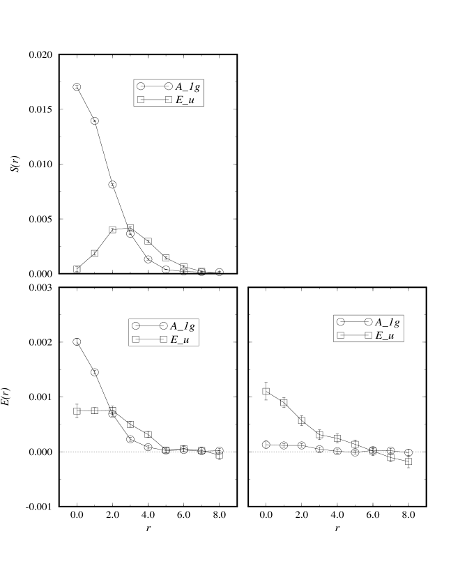
Figure 1: The colour flux contributions corresponding to the action ($S$), longitudinal ($E_{L}$, left plot) and transverse energy ($E_{T}$, right plot) sum rules of Eqs. (3–5) for the static quark potential. These are shown in lattice units (with $a\approx 0.6$ GeV^-1) versus transverse distance $r$ at the mid-point ($r_{L}=R/2$) for separation $R=8$. The data are for the symmetric ground state (A_1g representation) and first gluonic excitation (E_u representation).

The interpretation of these results is facilitated by the sum rules. Consider an interquark potential given by $V(R)=e/R+KR+V_{0}$, where the coefficient $e\approx-0.25$ for the A_1g potential (this is the ‘Coulomb’ coefficient) while in string models we expect $e=\pi$ for the first excited string mode (which corresponds [8] to the E_u case). Then the ‘transverse energy’ sum rule [Eq. (5)] will relate the sum over transverse energy fluctuations to $e$. This explains the much larger transverse energy seen in Figure 1 for the excited gluonic case. The other two sum rules suggest that the action and longitudinal energy will have fairly similar contributions when summed over $r_{T}$ for the two cases (the left hand side is $2K$ in each case). In fact we see a flatter $r_{T}$ distribution for the E_u case but the integrals over $r_{T}$ are more alike. This flatter distribution in $r_{T}$ corresponds to a ‘fatter’ flux tube for the excited gluonic case. A more detailed discussion will be found in [14].

In a string model, such as the Isgur-Paton flux tube model [13], the excited modes of the string (which contribute to the E_u potential) have wavefunctions which are suppressed at $r_{T}=0$. This gives a ‘fatter’ distribution. Unfortunately, in the simplest such picture, this applies only to the transverse energy while the other two combinations (action and longitudinal energy) would be little changed.

In conclusion, lattice techniques are able to explore the structure of string-like states in both the ground state and excited states. This gives support for such a string-like picture in general terms but models are not yet successful at reproducing our results in detail.

The authors wish to acknowledge that these calculations were carried out at the Centre for Scientific Computing’s C94 in Helsinki and the RAL(UK) CRAY Y-MP and J90. This work is part of the EC Programme “Human Capital and Mobility” – project number ERB-CHRX-CT92-0051.

References

- [1] C. Michael, Nucl. Phys. B280 (1987) 13.
- [2] H. Rothe, Phys. Lett. B355 (1995) 260.
- [3] I. H. Jorysz and C. Michael, Nucl. Phys. B302 (1988) 448.
- [4] G. Bali, C. Schlichter and K. Schilling, Phys.Lett. B363 (1995) 196.
- [5] C. Michael, Phys.Rev. D53 (1996) 4102.
- [6] F. Karsch, Nucl. Phys. B205 (1982) 285.
- [7] L.A. Griffiths, C. Michael and P.E.L. Rakow, Phys. Lett. 129B, 351 (1983)
- [8] S. Perantonis and C. Michael, Nucl. Phys. B347, 854-68 (1990).
- [9] S. Perantonis, A. Huntley and C. Michael, Nucl. Phys. B326, 544 (1989)
- [10] J. Engels, F. Karsch and K. Redlich, Nucl. Phys. B435 (1995) 295.
- [11] G. Bali, K. Schilling and C. Schlichter, Phys. Rev. D51 (1995) 5165.
- [12] R.W. Haymaker, V. Singh and Y.Peng, Phys.Rev. D53 (1996) 389.
- [13] N. Isgur and J.E. Paton, Phys. Rev. D31, 2910 (1985)
- [14] A. M. Green, C. Michael and P. S. Spencer, ‘The Structure of Flux-tubes in ’ in preparation.