Instabilities and Non-Reversibility of Molecular Dynamics Trajectories

Abstract

The theoretical justification of the Hybrid Monte Carlo algorithm depends upon the molecular dynamics trajectories within it being exactly reversible. If computations were carried out with exact arithmetic then it would be easy to ensure such reversibility, but the use of approximate floating point arithmetic inevitably introduces violations of reversibility. In the absence of evidence to the contrary, we are usually prepared to accept that such rounding errors can be made small enough to be innocuous, but in certain circumstances they are exponentially amplified and lead to blatantly erroneous results. We show that there are two types of instability of the molecular dynamics trajectories which lead to this behavior, instabilities due to insufficiently accurate numerical integration of Hamilton’s equations, and intrinsic chaos in the underlying continuous fictitious time equations of motion themselves. We analyze the former for free field theory, and show that it is essentially a finite volume effect. For the latter we propose a hypothesis as to how the Liapunov exponent describing the chaotic behavior of the fictitious time equations of motion for an asymptotically free quantum field theory behaves as the system is taken to its continuum limit, and explain why this means that instabilities in molecular dynamics trajectories are not a significant problem for Hybrid Monte Carlo computations. We present data for pure $SU(3)$ gauge theory and for QCD with dynamical fermions on small lattices to illustrate and confirm some of our results.

1 Introduction

The goal of this paper is to study the effect of errors introduced by working with finite-precision arithmetic on Hybrid Monte Carlo (HMC) and related algorithms.

The HMC algorithm [1, 2, 3] allows us to generate an ensemble of field configurations which are selected from some probability distribution. The algorithm is “exact,” in the sense that it is a Markov process which converges to the desired distribution with no systematic errors provided that the fictitious time molecular dynamics (MD) trajectories within it are exactly reversible and area preserving, that the computation of the action for the Metropolis accept/reject step is exact, and that we have a supply of perfectly random numbers. It does not require that the MD integration or any conjugate gradient (CG) “inversion” of the fermionic kernel be carried out exactly. Indeed, if we were to carry out all computations using exact arithmetic (i.e., with no rounding errors whatsoever) then the leapfrog integration scheme provides a method of integrating Hamilton’s equations while maintaining exact reversibility and area preservation.

All numerical computations carried out using floating point arithmetic are subject to rounding errors, but unless these errors are amplified exponentially we do not normally consider them to be a serious problem. The reason for this is that if a sensible rounding mode is used for the elementary floating point operations then the error after a sequence of $N$ operations, each of which gives rise to an error of magnitude $\varepsilon$, is $\varepsilon\sqrt{N}$. The cost of working with $d$ fractional digits grows approximately linearly with $d$ and gives $\varepsilon=10^{-d}$. Therefore if we require an answer with an error smaller in magnitude than $\delta$ in magnitude the cost is proportional to $-\log_{10}(\delta/\sqrt{N})$, which grows only like $\ln N$. This is a very small correction to the growth of the cost of the HMC algorithm as the volume and correlation length of the system is increased.

All the arguments we present as to the conditions under which reversibility is maintained apply to area preservation as well, but we shall concentrate on the former as the latter is less easy to determine empirically.

2 A Brief Survey of Algorithms

Let us very briefly summarize the various advantages and disadvantages of several variants of the HMC algorithm for dynamical fermion Quantum Chromodynamics (QCD) computations.

2.1 Hybrid Monte Carlo (HMC)

The algorithm is exact even if only a cheap approximate CG solution is carried out for computing the force along a MD trajectory, and such a CG solution is needed once per integration step. Nevertheless, an accurate CG solution is needed for the Metropolis accept/reject test once per trajectory.

If we believe that the behavior of free field theory carries over to interacting theories like QCD, then choosing trajectory lengths which grow linearly with the correlation length of the system $\tau\propto\xi$ minimizes the cost per independent configuration and give a dynamical critical exponent $z\approx 1$. The coefficient of proportionality depends upon which operator is being optimized, but it will typically be of order unity.

2.2 Second Order Langevin Monte Carlo (L2MC)

This algorithm was introduced by Horowitz [4] (and is sometimes also called Kramers algorithm). It is similar to HMC except that only single step (Langevin) trajectories are taken, and that instead of choosing the fictitious momenta from a Gaussian heatbath after each step the final momenta of a trajectory are reversed and mixed with a small amount of Gaussian noise to serve as the initial momenta for the next trajectory.

The advantages are that because the trajectories are short they are not subject to any large exponential amplification of rounding errors (which will be discussed in this paper), and that the the free field theory mean acceptance rate per trajectory is $\mathop{\rm erfc}(c\sqrt{V\delta\tau^{6}})$ whereas for HMC it is $\mathop{\rm erfc}(c^{\prime}\sqrt{V\delta\tau^{4}})$, where $V$ is the number of lattice sites, $\delta\tau$ is the leapfrog integration step size, and $c$ and $c^{\prime}$ are constants of order unity [5, 6, 7, 8].

The disadvantages are that an accurate CG solution is required for every integration step (because each such step has an accept/reject test following it), and that upon a rejection the trajectory reverses itself (because the momenta are flipped). This last observation means that in order to minimize autocorrelations the acceptance rate has to be very close to one with a concomitantly tiny $\delta\tau$.

A free field theory analysis [7, 8] indicates that L2MC and HMC have essentially the same scaling behavior in both the thermodynamic and continuum limits, so the choice between them must be made on the grounds of the cost of specific implementations and on the possible costs associated with instabilities occurring for long trajectories in HMC.

2.3 Generalized Hybrid Monte Carlo (GHMC)

The Generalized Hybrid Monte Carlo (GHMC) algorithm [9, 8] combines the HMC and L2MC methods giving an algorithm with three tunable parameters: the trajectory length $\tau$, the mixing angle between the old fictitious momenta and Gaussian noise $\theta$, and the integration step size $\delta\tau$. A free field theory analysis indicates that if $\delta\tau$ is chosen to given a good acceptance rate then there is a valley in the $(\tau,\theta)$ plane for which the dynamical critical exponent $z=1$ and furthermore for which the cost per independent configuration does not vary much.

As HMC and L2MC are both special cases of GHMC, the optimal choice of parameters may well not correspond to either case but in fact be somewhere in the middle of this valley.

3 Causes of Irreversibility

Empirical studies [10, 11] have shown that HMC computations for gauge theories are not exactly reversible. Given that they are performed using floating point arithmetic this is not at all surprising. However, if $\delta\tau$ or, for dynamical fermion calculations, the CG residual are taken to be too large then very large violations of reversibility are observed. This large violation of reversibility was observed even when the initial CG vector was chosen to be zero.

We recall that the HMC algorithm is exactly reversible unless the initial CG vector is chosen in a time asymmetric way except for the effects of finite-precision arithmetic. We are thus presented with the question of why the rounding errors are amplified by a large factor.

Three possible causes of this amplification suggest themselves:

• A small error changes the Metropolis accept/reject choice;

• A small error changes the number of CG iterations;

• The MD trajectories exhibit an exponential sensitivity to initial conditions (in other words they are unstable or chaotic) [11, 12].

It is easy to see that although the first two mechanisms produce a large change they occur correspondingly infrequently, and therefore are not compatible with the nature of the irreversibility observed. We therefore conclude that the irreversibility observed is caused by instabilities in the MD trajectories.

One may wonder to what extend irreversibility introduces systematic errors into the results of an HMC calculation. If the irreversibility is due to some underlying chaos in the equations of motion perhaps this just has the same effect as a different choice of random numbers for the fictitious momentum heatbath? Indeed, it is hard to see significant effects on physical observables unless truly huge violations of reversibility are induced (in which case the trajectories often become so unstable as to cause numerical overflows). We did observe that when the trajectories become irreversible there is often a large change in the fictitious kinetic energy as well (even though the total fictitious energy ${\delta H}$ stays small). This means that the distribution of fictitious momenta is clearly wrong, and thus the computation is erroneous even if the effect on physically interesting observables is hard to detect.

4 Causes of Instability

There are two distinct mechanisms which cause the MD equations to become unstable:

• The discrete integration procedure (leapfrog) diverges exponentially from solutions of the classical equations of motion. This instability should grow with the number of integration steps, and thus have a short characteristic time scale for large volumes.

• The classical equations of motion are themselves chaotic. These may be expected to have a time scale independent of the step size, and presumably determined by some characteristic length scale of the system.

In section 5 we analyze the instabilities of the leapfrog integration scheme for free field theory, and in section 6 we consider the chaotic nature of the underlying continuous time equations of motion themselves and propose a hypothesis as to how the time scale of the corresponding instabilities behaves as the system approaches the continuum limit.

5 Free Field Theory Analysis

The phenomenon of the leapfrog integration scheme diverging from the true trajectory occurs even for free field theory, and it is instructive to see what happens there [7, 8].

Consider a system of harmonic oscillators $\{\phi_{p}\}$ for $p\in{\bbxii Z}_{V}$. The Hamiltonian on fictitious phase space is

$$H={\scriptstyle{1\over 2}}\sum_{p\in{\bbxii Z}_{V}}\left(\pi_{p}^{2}+\omega_{p}^{2}\phi_{p}^{2}\right).$$

5.1 Single Mode Analysis

The Hamiltonian is diagonal, so we may temporarily consider the evolution of a single mode and set its frequency $\omega_{p}=1$. In fact, we will find that the essential features of the instability are displayed by a single mode.

The leapfrog discretization of Hamilton’s equations can be written as the following matrix acting on the phase space vector $(\phi,\pi)$

$$U(\delta\tau)=\left(\begin{array}[]{cc}1-{\scriptstyle{1\over 2}}\delta\tau^{2}&\delta\tau\\ -\delta\tau+{\scriptstyle{1\over 4}}\delta\tau^{3}&1-{\scriptstyle{1\over 2}}\delta\tau^{2}\end{array}\right).$$

The general area-preserving reversible linear map on $(\phi,\pi)$ phase space may be parameterized as

$$U(\delta\tau)=\left(\begin{array}[]{cc}\cos[\kappa(\delta\tau)\delta\tau]&{\displaystyle\sin[\kappa(\delta\tau)\delta\tau]\over\displaystyle\rho(\delta\tau)}\\ -\rho(\delta\tau)\sin[\kappa(\delta\tau)\delta\tau]&{\cos[\kappa(\delta\tau)\delta\tau]}\end{array}\right),$$

where $\kappa$ and $\rho$ are even functions, but not necessarily real valued. For the lowest-order leapfrog algorithm $\kappa$ and $\rho$ are

$$\kappa(\delta\tau)={\cos^{-1}(1-{\scriptstyle{1\over 2}}\delta\tau^{2})\over\delta\tau},\qquad\rho(\delta\tau)=\sqrt{1-{\scriptstyle{1\over 4}}\delta\tau^{2}}.$$

With this parameterization it is easy to see that the evolution operator for a trajectory of $\tau/\delta\tau$ leapfrog steps is

$$U(\tau)=\left(\begin{array}[]{cc}\cos[\kappa(\delta\tau)\tau]&{\displaystyle\sin[\kappa(\delta\tau)\tau]\over\displaystyle\rho(\delta\tau)}\\ -\rho(\delta\tau)\sin[\kappa(\delta\tau)\tau]&{\cos[\kappa(\delta\tau)\tau]}\end{array}\right),$$

and thus the change in fictitious energy over this trajectory is

$${\delta H}={1\over 2}\sum_{p\in{\bbxii Z}_{V}}\left(\begin{array}[]{c}\phi_{p}\\ \pi_{p}\end{array}\right)^{T}\Bigl{[}U_{p}^{T}U_{p}-{\bbxii I}\Bigr{]}\left(\begin{array}[]{c}\phi_{p}\\ \pi_{p}\end{array}\right).$$

It is clear that some kind of critical behavior will occur at $\delta\tau=2$.

Given this evolution matrix we can compute the probability distribution of ${\delta H}$,

$$P_{\delta H}(\xi) = {1\over Z}\int[d\phi][d\pi]e^{-H}\delta(\xi-{\delta H})={1\over Z}\int[d\phi][d\pi]e^{-H}\int_{-\infty}^{\infty}{d\eta\over 2\pi}\,e^{i\eta(\xi-{\delta H})}$$ (1)

$$= \int_{-\infty}^{\infty}{d\eta\over 2\pi}\,{e^{i\eta\xi}\over\prod_{p}\sqrt{\det[{\bbxii I}+i\eta(U_{p}^{T}U_{p}-{\bbxii I})]}}=\int_{-\infty}^{\infty}{d\eta\over 2\pi}\,{e^{i\eta\xi}\over\prod_{p}\sqrt{1+T_{p}^{2}i\eta(1-i\eta)}}$$

where $T\equiv\left|\left(\rho-{\displaystyle 1\over\displaystyle\rho}\right)\sin(\kappa\tau)\right|$. It is easy to see that $T$ rapidly approaches its asymptotic behavior of growing proportionally to $e^{\nu\tau}$ where

$$\nu=\pm{1\over\delta\tau}\mathop{\rm Re}\ln\left[{\scriptstyle{1\over 2}}\delta\tau^{2}-1\pm\delta\tau\sqrt{{\scriptstyle{1\over 4}}\delta\tau^{2}-1}\right],$$ (2)

(which falls as $2\ln(\delta\tau)/\delta\tau$ as $\delta\tau\to\infty$). For $\delta\tau\leq 2$ not only is the exponent $\nu$ zero, but $T$ is bounded by a constant. That the exponent decreases as $\delta\tau\to\infty$ merely reflects the fact that $T$ is growing exponentially in the number of MD steps but only algebraically in the step size $\delta\tau$. This is illustrated in Figure 1.

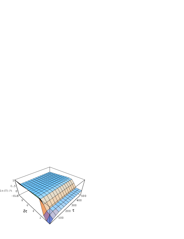
Figure 1: The “exponent” $\mathop{\rm Re}\ln(T)/\tau$ is shown as a function of the integration step size $\delta\tau$ and the trajectory length $\tau$. This quantity approaches $\nu$ as $\tau\to\infty$.

For a single mode the probability distribution of ${\delta H}$ may be evaluated by changing variable to $\eta^{\prime}\equiv\eta+i/2$

$$P_{\delta H}(\xi)=\int_{-\infty}^{\infty}{d\eta\over 2\pi}\,{e^{i\eta\xi}\over\sqrt{1+T^{2}i\eta(1-i\eta)}}=e^{\xi/2}\int_{i/2}^{\infty+i/2}{d\eta^{\prime}\over\pi}\,{\cos(\eta^{\prime}\xi)\over\sqrt{1+T^{2}({\scriptstyle{1\over 4}}+\eta^{\prime 2})}}.$$ (3)

The singularities in the integrand occur when $1+T^{2}({\scriptstyle{1\over 4}}+\eta^{\prime 2})=0$, for which $\eta^{\prime 2}<-{\scriptstyle{1\over 4}}$ and hence $|\mathop{\rm Im}\eta^{\prime}|>{\scriptstyle{1\over 2}}$. We may thus shift the integration contour to the real axis, and defining $x\equiv T\eta^{\prime}/\sqrt{1+{\scriptstyle{1\over 4}}T^{2}}$ we obtain

$$P_{\delta H}(\xi)={e^{\xi/2}\over\pi T}\int_{0}^{\infty}{dx\over\sqrt{1+x^{2}}}\cos\left({x\xi\over 2}\sqrt{1+{4\over T^{2}}}\right),$$

which can be expressed in closed form in terms of a modified Bessel function

$$P_{\delta H}(\xi)={e^{\xi/2}\over\pi T}K_{0}\left({|\xi|\over 2}\sqrt{1+{4\over T^{2}}}\right).$$

The logarithm of the acceptance rate is shown in Figure 2.

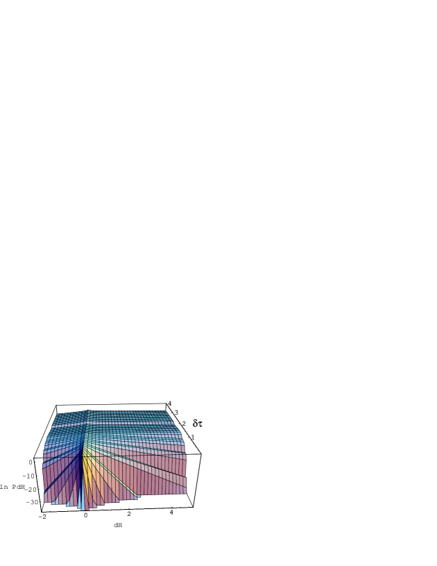
Figure 2: The logarithm of the probability distribution for the change in fictitious energy ${\delta H}$ for a single mode is shown as a function of ${\delta H}$ and the MD leapfrog integration step size $\delta\tau$ for a trajectory of length $\tau=4$ (rounded to the nearest integer multiple of $\delta\tau$).

The average Metropolis acceptance rate is

$$P_{\hbox{\rm\tiny acc}}\equiv\Big{\langle}\min(1,e^{-{\delta H}})\Big{\rangle}=\int_{-\infty}^{\infty}d\xi\,\min(1,e^{-\xi})P_{\delta H}(\xi).$$ (4)

For a single mode we may use eq. (3), and evaluating the integral over $\xi$ gives

$$P_{\hbox{\rm\tiny acc}}={2\over\pi T}\int_{-\infty}^{\infty}{dx\over\sqrt{1+x^{2}}\left[1+x^{2}\left(1+{4\over T^{2}}\right)\right]};$$

setting $x\equiv{1\over 2}\left(\sqrt{y}-{\displaystyle 1\over\displaystyle\sqrt{y}}\right)$ and ${2\over T}\equiv\tan{\theta\over 2}$ we easily obtain

$$P_{\hbox{\rm\tiny acc}}={\sin\theta\over\pi}\int_{0}^{\infty}{dy\over y^{2}+2y\cos\theta+1}={\theta\over\pi}={2\over\pi}\tan^{-1}\left({2\over T}\right),$$

and this is shown in Figure 3 as a function of the step size and trajectory length. Observe that there is a “wall” at $\delta\tau=2$ which separates the region where the acceptance rate oscillates as a function of $\tau$ from the region where it plummets exponentially.

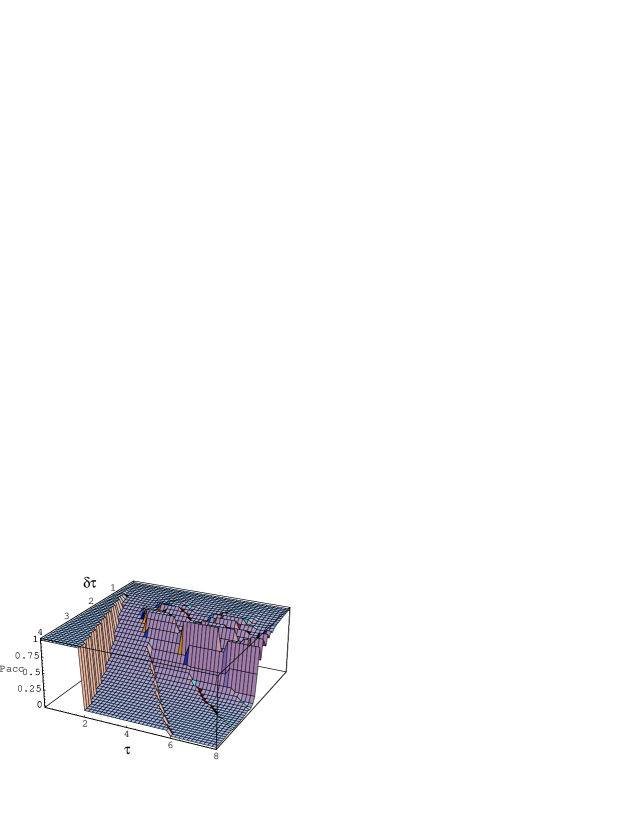
Figure 3: Acceptance rate for a single mode as a function of the MD step size $\delta\tau$ and trajectory length $\tau$ (rounded to the nearest integer multiple of $\delta\tau$).

5.2 Multiple Mode Analysis

These results can be generalized to a field theory with many “stable” modes and some number of “unstable” ones. In the general case let us consider the acceptance rate $P_{\hbox{\rm\tiny acc}}$ defined in eq. (4) and use the expression of eq. (1) for the distribution of values of ${\delta H}$. As before we may make the change of variable $\eta^{\prime}\equiv\eta+i/2$ and observe that there are no singularities in the strip of the complex $\eta^{\prime}$ plane satisfying $|\mathop{\rm Im}\eta^{\prime}|<{\scriptstyle{1\over 2}}$. We thus obtain

$$P_{\hbox{\rm\tiny acc}} = \int_{-\infty}^{0}d\xi\,P_{\delta H}(\xi)+\int_{0}^{\infty}d\xi\,P_{\delta H}(\xi)e^{-\xi}$$

$$= \int_{-\infty}^{\infty}{d\eta^{\prime}\over 2\pi}\,{1\over\prod_{p}\sqrt{1+T_{p}^{2}({\scriptstyle{1\over 4}}+\eta^{\prime 2})}}\left[\int_{-\infty}^{0}d\xi\,e^{(i\eta^{\prime}+{\scriptstyle{1\over 2}})\xi}+\int_{0}^{\infty}d\xi\,e^{(i\eta^{\prime}-{\scriptstyle{1\over 2}})\xi}\right]$$

$$= \int_{-\infty}^{\infty}{d\eta^{\prime}\over 2\pi}\,{1\over({\scriptstyle{1\over 4}}+\eta^{\prime 2})\prod_{p}\sqrt{1+T_{p}^{2}({\scriptstyle{1\over 4}}+\eta^{\prime 2})}}.$$

Let us now assume that there are a small number $N$ of “unstable” modes with $T_{q}\gg 1$ and a large number $V$ of “stable” modes with $T_{p}\ll 1$ such that $\sum_{p=1}^{V}T_{p}^{2}\equiv\sigma^{-2}$ and $\sum_{p=1}^{V}T_{p}^{2n}=O(V^{1-n})$. We can thus compute an asymptotic expansion valid for large $V$,

$$P_{\hbox{\rm\tiny acc}} = \int_{-\infty}^{\infty}{d\eta^{\prime}\over 2\pi}\,{\exp\left\{-{\scriptstyle{1\over 2}}\sum_{p=1}^{V}\ln\left[1+T_{p}^{2}({\scriptstyle{1\over 4}}+\eta^{\prime 2})\right]\right\}\over({\scriptstyle{1\over 4}}+\eta^{\prime 2})\prod_{q=1}^{N}\sqrt{1+T_{q}^{2}({\scriptstyle{1\over 4}}+\eta^{\prime 2})}}$$

$$\sim e^{-1/8\sigma^{2}}\int_{-\infty}^{\infty}{d\eta^{\prime}\over 2\pi}\,{e^{-\eta^{\prime 2}/2\sigma^{2}}\over({\scriptstyle{1\over 4}}+\eta^{\prime 2})\prod_{q}\sqrt{1+T_{q}^{2}({\scriptstyle{1\over 4}}+\eta^{\prime 2})}}\biggl{(}1+{\scriptstyle{1\over 4}}\sum_{p}T_{p}^{4}({\scriptstyle{1\over 4}}+\eta^{\prime 2})^{2}+\cdots\biggr{)},$$

where the “stable” modes correspond to subscript $p$ and the unstable ones to subscript $q$. If there are a few modes with $V^{-1/4}\ll\omega_{p}\delta\tau\ll 1$ then these may be taken into account by computing further terms in the asymptotic expansion above. On the other hand, we may carry out an expansion in powers of $1/T_{q}$ for the “unstable” modes by writing

$${1\over\prod_{q=1}^{N}\sqrt{1+T_{q}^{2}({\scriptstyle{1\over 4}}+\eta^{\prime 2})}}={({\scriptstyle{1\over 4}}+\eta^{\prime 2})^{-N/2}\over\prod_{q}T_{q}}\biggl{(}1-{\scriptstyle{1\over 2}}\sum_{q}{1\over T_{q}^{2}}({\scriptstyle{1\over 4}}+\eta^{\prime 2})^{-1}+\cdots\biggr{)}.$$ (5)

Using this expansion in the integrand above reduces both the large $T$ and small $T$ expansions to a sum of integrals of the form

$$\int_{0}^{\infty}d\eta^{\prime}\,e^{-\eta^{\prime 2}/2\sigma^{2}}({\scriptstyle{1\over 4}}+\eta^{\prime 2})^{-k/2}=2^{k-2}\sqrt{\pi}U\Bigl{(}{1\over 2},{3-k\over 2};{1\over 8\sigma^{2}}\Bigr{)}$$ (6)

where $U$ is a confluent hypergeometric function. It is easily verified that for $N=0$ the leading term in the asymptotic expansion is just $\mathop{\rm erfc}(1/\sqrt{8\sigma^{2}})$.

In Figure 4 we show the $P_{\hbox{\rm\tiny acc}}$ for the case where there are many “stable” modes with $\sigma=1$ as a function of the value of $\sigma$ for one additional “unstable” mode. It is clear that the expansions calculated above are very good as long as $T$ is not close to one.

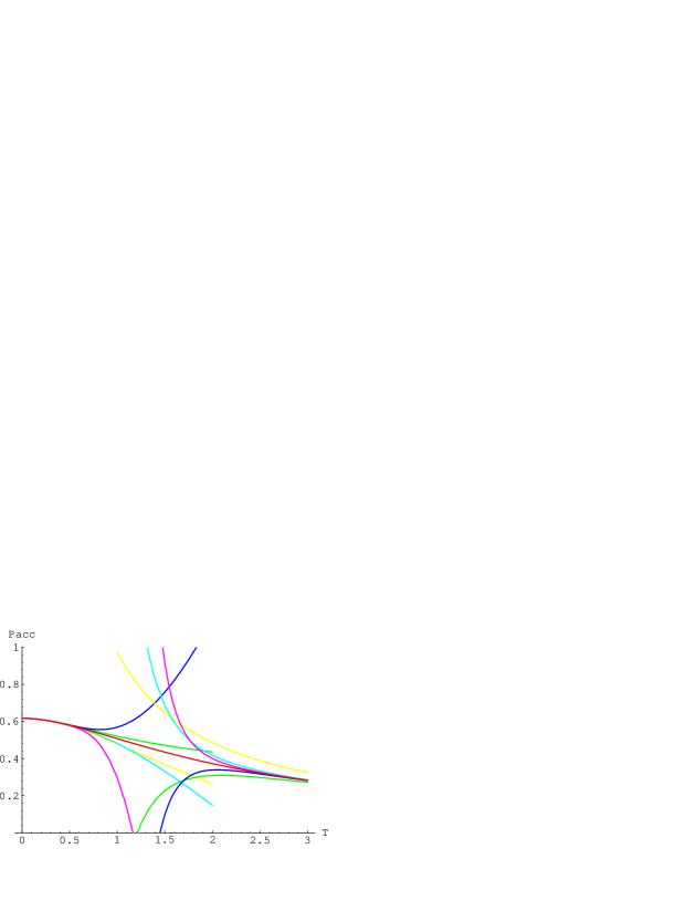
Figure 4: Acceptance rate for many “stable” modes with $\sigma=1$ and one “unstable” mode as a function of the value of $T$ for the “unstable” mode. In addition to the result obtained by numerical integration various orders of the small- and large-$T$ expansions are shown.

In Figure 5 we plot $\ln P_{\hbox{\rm\tiny acc}}$ as a function of $T$ for various values of $N$, the number of “unstable” modes. Each additional unstable mode clearly reduces the acceptance rate by a large factor for these parameters, and this makes it reasonable to assume that at least the qualitative behavior of the instabilities in the system is apparent from the case where there is just a single unstable mode.

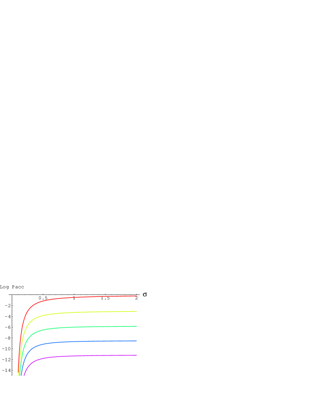
Figure 5: Logarithm of the mean acceptance rate for $N$ “unstable” modes as a function of $\sigma$ for $T=25.63$ which corresponds to $\delta\tau=2.1$ and $\tau=9$. The four curves are for $N$ from $0$ (top) to $4$ (bottom).

In Figure 6 we show a comparison of the dependence of the mean acceptance rate on $T$ for a single mode and for a system of many “stable” modes and one “unstable” one. This demonstrates that the behavior of a single mode dominates the instabilities in the case of free field theory.

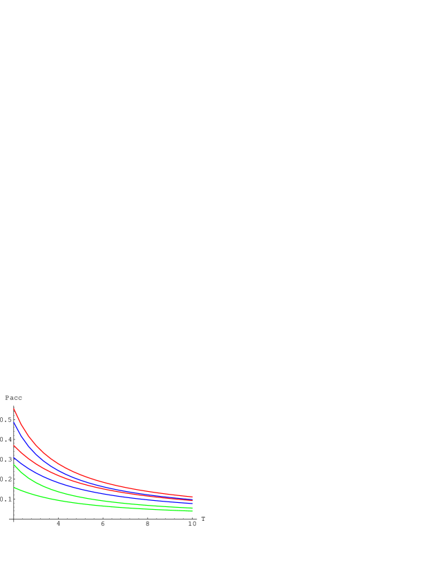
Figure 6: Comparison of the acceptance rate for a single mode (multiplied by a factor of $\mathop{\rm erfc}(1/\sqrt{8\sigma^{2}})$ compared with the corresponding acceptance rate for one “unstable” mode and many “stable” modes for $\sigma=0.5$, $1$, and $1.5$.

We notice that in order to keep the acceptance rate constant as the lattice volume $V\to\infty$ we must decrease $\delta\tau$ so as to keep $V\delta\tau^{4}$ fixed. Thus as we approach the thermodynamic limit the instabilities will go away: in other words the leapfrog instability is a finite volume effect.

5.3 Interacting Field Theories

When interactions are present it is no longer meaningful to talk of independent modes, but for weak interactions like those for asymptotically free field theories at short distance it is still useful to consider the system as a set of weakly coupled modes. We expect that the onset of the integration instability will still be caused by the highest frequency mode, and will occur at $\omega_{\max}\delta\tau=2$. The forces acting on the highest frequency mode due to the other modes will fluctuate in some complicated way, and consequently we would expect that the “wall” at $\omega_{\max}\delta\tau=2$ gets smeared out.

In order to illustrate this effect we have made numerical studies of a simple model of a single harmonic oscillator whose frequency is randomly chosen from a Gaussian distribution with mean unity and standard deviation $\sigma$ before each MD step. The behavior of this model is just like that of the free field theory considered above, except that the “wall” at $\delta\tau=2$ gets spread out. Our numerical results are shown in Figure 7, where the analytic result for $\sigma=0$ is taken from eq. (2).

Figure 7: Results from fluctuating-frequency harmonic oscillator model. The curve for $\sigma=0$ is given by eq. (2) on page 2.

We conjecture that interacting asymptotically free field theories like non-Abelian gauge theories behave similarly, and this is supported by our numerical results.

We do not expect the introduction of dynamical fermions to produce any qualitatively different behavior. For QCD computations using the HMC algorithm the pseudofermions produce a force which we expect to be proportional to $1/m_{f}$, so the “highest frequency” of the system, which is responsible for the integration instability, will grow as $\omega_{\max}\propto 1/m_{f}$ too. In particular we expect $\omega_{\max}$ to become large as $m_{f}\to 0$, so the critical value of $\delta\tau$ will become small as $\kappa\to\kappa_{c}$ for Wilson fermions. An inaccurate CG solution will produce errors which are multiplied by the scale of this fermionic force, and will become important when the size of the errors in the CG solution become comparable with the size of the fluctuations in the forces due to the fields themselves.

It is interesting to observe that reversibility can be violated significantly even though the acceptance rate does not become small. For example we will see an example of this in Figure 10 on page 10 for $\delta\tau=0.005$ and $\tau=50$. This is because the leapfrog integration scheme tries to conserve energy even when it has wandered far away from the true continuous time trajectory. It is therefore prudent to verify that reversibility is satisfied to the precision required, even when the HMC algorithm has an average acceptance rate which is close to one.

6 Chaos in Continuous Time Evolution

Jansen and Liu [11] observed that there is a second cause of instability in the MD trajectories, which occurs even when the integration step size $\delta\tau\to 0$. This is because the underlying continuous fictitious time equations of motion are themselves chaotic. In the chaotic regime two nearby classical trajectories diverge exponentially with a characteristic exponent $\nu$ called the Liapunov exponent. Obviously such behavior cannot be studied in the context of free field theory.

The instability due to chaos cannot be removed by reducing $\delta\tau$, and is therefore not a finite size effect. If the system we are studying exhibits critical slowing down, and we believe that the mechanism for reducing this to $z=1$ in free field theory is applicable to this system too, and we wish to use the HMC algorithm, then we must scale the trajectory length with the correlation length, $\tau\propto\xi$. This means that there is the potential for exponential amplification of rounding errors.

Even if there is such an exponential amplification of rounding errors, reversibility can be maintained to any desired precision by a linear increase in the number of digits used for floating point arithmetic. This is no longer a negligible addition to the computational complexity of the problem (i.e., it is not just a logarithmic correction), but it is still a small correction to the power dependence of the computational cost on the correlation length and volume.

This problem can be avoided using the GHMC algorithm, but not only is this unnecessary until chaotic amplification of rounding errors becomes important, but also as we shall see it might never be necessary at all.

The reason for this is that the Liapunov exponent (averaged over the equilibrium distribution) is not constant as a function of $\beta$. If the chaotic dynamics is not only a property of the underlying continuous fictitious time evolution, but is also a property of the underlying (space-time) continuum field theory, then the Liapunov exponent would be constant when measured in “physical” units, that is $\nu\xi$ would be constant as $\xi\to\infty$. In other words this hypothesis would say that $\nu\propto 1/\xi$, or for QCD with $n_{f}$ flavors of fermions

$$\nu\propto e^{-\beta/12\beta_{0}}\qquad\hbox{\rm with}\qquad\beta_{0}={11-{2\over 3}n_{f}\over 16\pi^{2}},$$ (7)

where the last relation follows from perturbation theory for $\beta$ large enough that the system exhibits asymptotic scaling. In section 7.2 we shall present numerical evidence that this hypothesis may indeed be true. If this is the case, then tuning the HMC algorithm by varying the trajectory length proportionally to the correlation length does not lead to any change in the amplification of rounding errors as we change $\xi$.

7 Monte Carlo Results

We have carried out extensive numerical studies of reversibility errors for (quenched) $SU(3)$ gauge theory and for full QCD with two flavors of dynamical Wilson fermions. Measurements were made principally on $4^{4}$ lattices, but additional data on $8^{4}$ lattices was used for an analysis of finite size effects.

7.1 Numerical Determination of Reversibility Errors

In order to measure the deviation from reversibility of MD trajectories we chose some initial point in fictitious phase space $(U_{i},\pi_{i})$ and followed an MD trajectory of length $\tau$ to the final point $(U_{f},\pi_{f})$; we then reversed the fictitious momenta and followed the backward trajectory of length $\tau$ from $(U_{f},-\pi_{f})$ to $(U^{\prime}_{i},\pi^{\prime}_{i})$. At the end of this backward trajectory we measured the amount by which it failed to return to its starting point by computing two quantities, the change in energy $\Delta\delta H\equiv H(U_{i}^{\prime},\pi_{i}^{\prime})-H(U_{i},\pi_{i})$, and the norm of the change in the gauge field $||\Delta\delta U||\equiv||U_{i}^{\prime}-U_{i}||$, where $||U||^{2}\equiv\sum_{x,\mu}\sum_{a,b}\Bigl{|}[U_{\mu}(x)]_{ab}\Bigr{|}^{2}$, $a$ and $b$ being $SU(3)$ color indices. Observe that both quantities are extensive in the lattice volume, that $\Delta\delta H$ is gauge invariant whereas $||\Delta\delta U||$ is not, and that $||\Delta\delta U||$ cannot be small unless $\Delta\delta H$ is too. These quantities can also be considered as the difference between the change in energy or gauge field over the forward and the backward trajectories, which serves to explain our notation. Both of these quantities vanish identically for reversible trajectories, of course.

7.1.1 $SU(3)$ Gauge Theory

For $SU(3)$ gauge theory an example of a long trajectory is shown in Figure 8. This shows how the energy ${\delta H}$ changes along a long trajectory. The change in energy over the forward trajectory was ${\delta H}=1.2$ (corresponding to an acceptance probability of 30%), which differed from the change in energy over the backward trajectory by $\Delta\delta H=0.36$. This clearly shows that the leapfrog integration scheme tries very hard to conserve energy even though it has wandered far from the true path: indeed, the backward trajectory ends up a distance $||\Delta\delta U||=20$ away from the starting configuration.

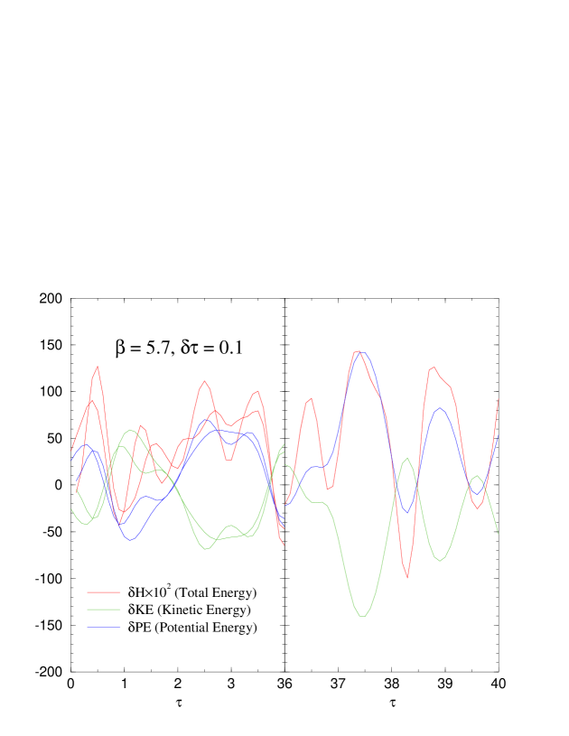
Figure 8: The contributions to ${\delta H}$ from the fictitious kinetic energy and the potential energy (gauge action) for a trajectory of length $\tau=40$ with step size $\delta\tau=0.1$ at $\beta=5.7$. The two graphs show the contributions to the energy for the first and last four units of fictitious time respectively, overlaid with the corresponding quantities on the backward trajectory. The graph on the right shows that the forward are backward trajectories are essentially indistinguishable immediately after the reversal, and the graph on the left shows how the backward trajectory finally deviates from the forward one. Note that the cancellation between $\delta$KE and $\delta$PE is still at the 2% level even at the end of this very long trajectory with large step size, as the ${\delta H}$ values have been multiplied by a factor of 100.

This example demonstrates that there can be severe violations of reversibility even though the acceptance rate is quite reasonable, but it should be noted that a trajectory length of $\tau=40$ is unreasonably long for a system whose correlation length $\xi=O(1)$, especially on a $4^{4}$ lattice!

By carrying out such forward and backward trajectories for a variety of step sizes and trajectory lengths we produced Figures 9 and 10.

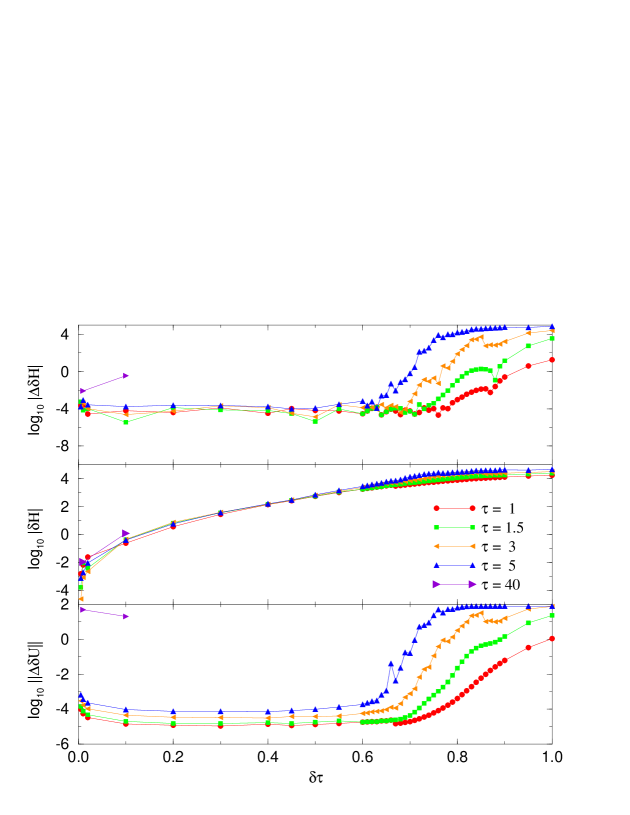
Figure 9: Results for pure $SU(3)$ gauge theory with $\beta=5.7$ on a $4^{4}$ lattice as a function of $\delta\tau$.

In the former we plot the logarithm of $|\Delta\delta H|$, $|{\delta H}|$, and $||\Delta\delta U||$ as a function of the integration step size. The differences between measurements made on different equilibrated configurations were very small. The “kinks” in some of the curves are just a consequence of rounding $\tau$ to the nearest integer multiple of $\delta\tau$. The top and bottom graphs clearly show the integration instability “wall” at $\delta\tau\approx 0.6$, which has spread out just as we would expect. The middle graph shows that by the time one has reached the “wall” ${\delta H}=O(10^{3})$, so the integration instabilities are of no practical importance for this system. If one looks carefully at the left end of the bottom graph one sees that $||\Delta\delta U||$ increases a little as $\delta\tau\to 0$. This is because the number of integration steps $n=\tau/\delta\tau$ is increasing, and therefore rounding errors are being amplified by the usual $\sqrt{n}$ factor.

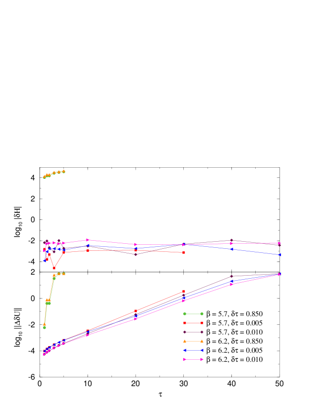
Figure 10: Results for pure $SU(3)$ gauge theory with $\beta=5.7$ and $6.2$ on a $4^{4}$ lattice as a function of $\tau$.

For extremely long trajectories reversibility is violated even for very small values of $\delta\tau$; in order to understand this it is instructive to look at Figure 10, where we plot the logarithm of ${\delta H}$ and $||\Delta\delta U||$ as a function of the trajectory length for two values of $\beta$ and three values of $\delta\tau$. The lower graph immediately shows us that even for very small step sizes the errors are amplified exponentially, with an exponent which is independent of $\delta\tau$ (i.e., the lines for the same $\beta$ value but different $\delta\tau$ are parallel). This is evidence for chaos in the continuous time equations of motion, as suggested by Jansen and Liu [11]. The lines for small step size on the lower graph eventually curve downwards for the largest $\tau$ values because $SU(3)$ is a compact manifold so there is a maximum distance two configurations can be from one another, and this bound is becoming saturated. The upper graph shows that ${\delta H}$ stays small for small $\delta\tau$ even though the rounding errors have been enormously amplified.

7.1.2 QCD with Wilson Fermions

We have carried out the corresponding analysis for full QCD with two flavors of Wilson fermions with configurations taken from two ensembles, one at $\beta=5.1$ and $\kappa=0.16$ which corresponds to quite heavy quarks, and one at $\beta=3.5$ and $\kappa=0.2225$ which is extremely close to $\kappa_{c}$. We took care that both ensembles were in the “confined phase,” if we use thermodynamic terminology to approximately describe the finite size effects on our symmetric lattices.

Figure 11 shows a typical trajectory for the light dynamical fermion system. For this trajectory ${\delta H}=3.9\times 10^{-2}$ corresponding to an acceptance probability of 96%, and $||\Delta\delta U||=1.4\times 10^{-2}$. This trajectory exhibits some typical behavior: the potential energy oscillates smoothly with a period of about $2$ MD time units; the fermionic energy is much more jittery; and the kinetic energy adjusts itself to cancel the other two components leaving a small residual ${\delta H}$ whose magnitude is about a percent of that of its constituent parts. The three constituent contributions to the energy are of similar magnitudes, which indicates that the fermions are indeed very light: with heavier fermions the fermionic energy is much smaller.

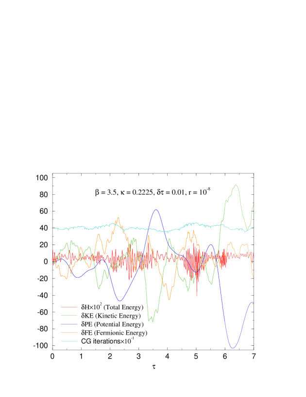
Figure 11: The contributions to ${\delta H}$ from the fictitious kinetic energy, potential energy (gauge action), and the fermionic energy for a trajectory of length $\tau=7$ with step size $\delta\tau=0.01$ at $\beta=3.5$ and $\kappa=0.2225$. Each curve is overlaid with the corresponding quantities on the backward trajectory, but the forward and backward trajectories are indistinguishable on this scale. Note that ${\delta H}$ has been scaled by a factor of 100 because it has a magnitude of less than a percent of its constituent parts. The number of CG iterations used to reach the residual $r=10^{-8}$ from a zero start is also shown (divided by a factor of 10).

From many such trajectories on several equilibrated configurations we produced the data shown in Figures 12 and 13. For simplicity we only show the data for the heavy fermion case in Figure 12. The results are very similar to the pure $SU(3)$ gauge theory results of Figures 9 and 10, especially if one notes that the trajectory lengths are somewhat longer in the present case.

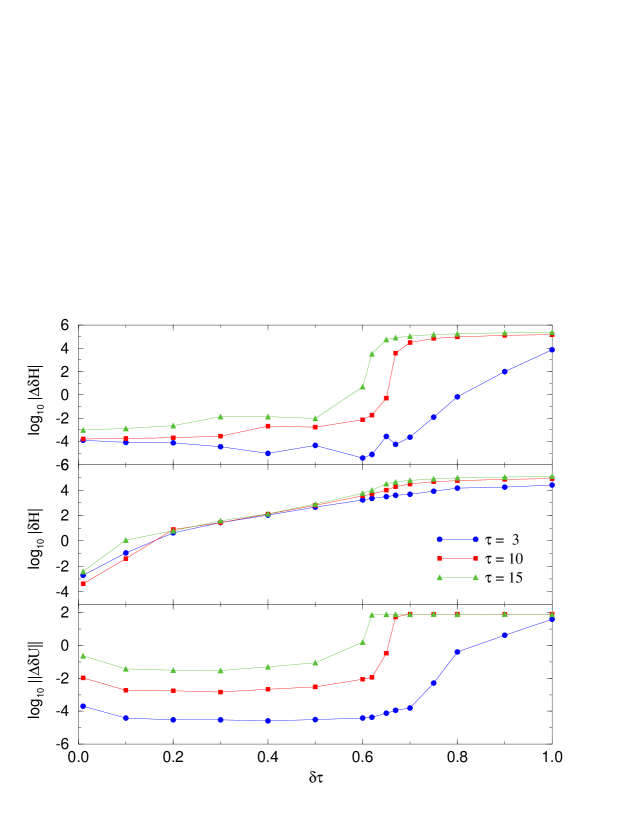
Figure 12: Results for QCD as a function of integration step size $\delta\tau$. The data shown is for $\beta=5.1$, $\kappa=0.16$, and CG residual $r=10^{-8}$ on a $4^{4}$ lattice.

Just as in that case we observe the smeared-out “wall” at which the leapfrog integration scheme becomes unstable, but that the acceptance rate is already completely negligible by the time the wall is reached. We also see that long trajectories with small step sizes exhibit chaotic behavior.

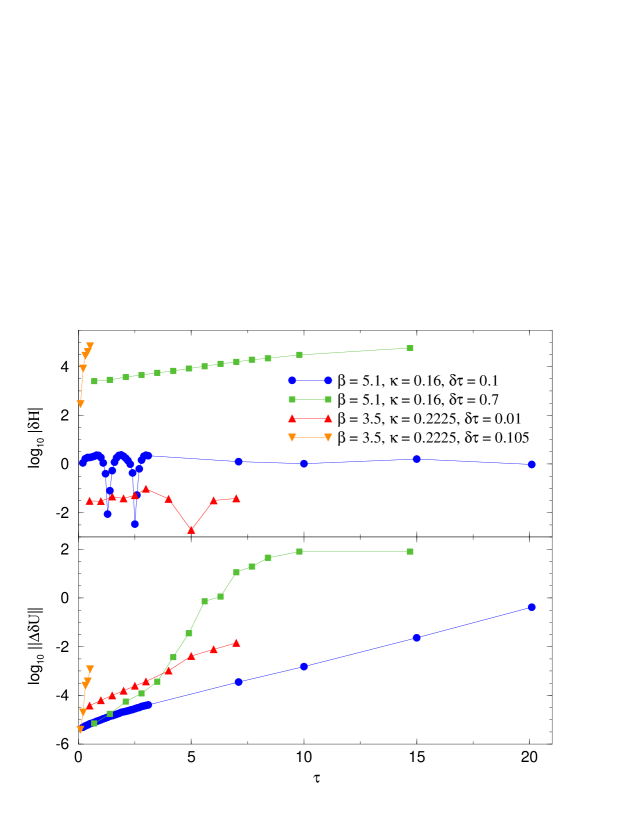
Figure 13: Results for QCD as a function of trajectory length $\tau$. The data shown is from $4^{4}$ lattices with a CG residual $r=10^{-8}$.

All our data show a clear exponential instability in $||\Delta\delta U||$ as a function of $\tau$, so we fitted the data over the range of $\tau$ for which this exponential behavior was obvious and extracted a characteristic exponent $\nu$ (which we shall henceforth call the Liapunov exponent, although this might not always be quite the correct terminology). In Figure 14 we show the Liapunov exponent as a function of the step size $\delta\tau$ for pure $SU(3)$ gauge theory, and QCD with heavy and light dynamical fermions.

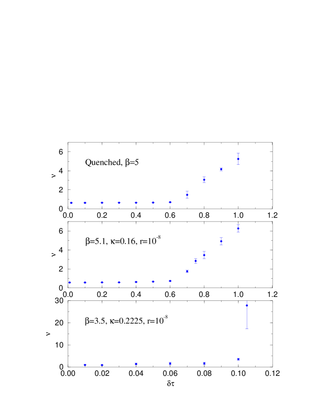
Figure 14: The Liapunov exponent $\nu$ is shown as a function of the integration step size $\delta\tau$. The top graph is for pure $SU(3)$ gauge theory, the middle one is for QCD with heavy dynamical Wilson quarks, and the bottom one is for QCD with light dynamical Wilson quarks. Note that the scale for the light quark case is quite different from the other two. The error bars show the standard deviation of measurements made on three independent configurations.

The results show the same qualitative behavior as that of our toy model which was exhibited in Figure 7 on page 7, except that

• The “wall” where the integration instability sets in is at a different value of $\delta\tau$ (about $0.6$ for the pure gauge theory and heavy fermion cases, and about $0.1$ for the light fermion case). This probably just reflects the different highest frequencies of the systems.

• The exponent is not zero for small $\delta\tau$, but has some fixed non-vanishing value. This is just the evidence for chaotic continuous time dynamics discussed earlier.

The integration instability is easily avoided by choosing a sufficiently small step size, which is forced upon us anyhow as the lattice volume becomes large if we want to maintain a reasonable Metropolis acceptance rate. This, of course, is exactly what we mean by saying that the integration instability is a finite volume effect. Furthermore, it is clear that even a $4^{4}$ lattice is sufficiently large for us to be driven well away from the “wall” for all the parameters we have considered.

We shall therefore turn our attention to the chaotic instability which is present for any value of $\delta\tau$, and in the next section we shall investigate the dependence of $\nu$ upon the parameters of our lattice field theories.

7.2 Parameter Dependence of Liapunov Exponent

We investigated the dependence of the Liapunov exponent $\nu$ on the coupling constant $\beta$ for pure $SU(3)$ gauge theory. The results are shown in Figure 15 and 16. In the former we plot $\ln||\Delta\delta U||$ against $\tau$ for a variety of values of $\beta$. All of the curves exhibit a very clear exponential instability: for small $\beta$ the relation is almost completely linear on this semi-logarithmic plot, whereas for large $\beta$ there is some initial curvature before a linear region is reached. The slope (i.e., the Liapunov exponent) decreases very rapidly between $\beta=5.4$ and $6.0$, which is just below the finite-size analogue of the finite temperature deconfinement transition on a $8^{4}$ lattice.

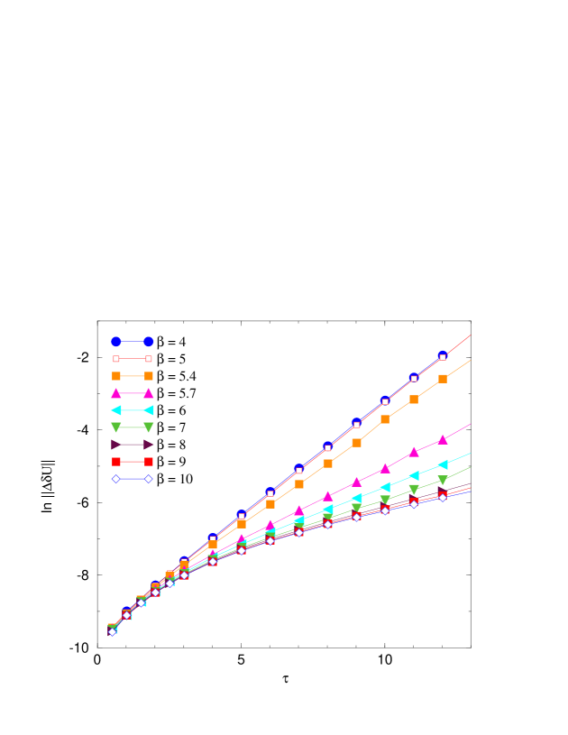
Figure 15: $||\Delta\delta U||$ as a function of trajectory length $\tau$ for a variety of values of $\beta$ for pure $SU(3)$ gauge theory on $8^{4}$ lattices.

In Figure 16 we plot the measured values of the Liapunov exponent $\nu$ as a function of $\beta$ for both $4^{4}$ and $8^{4}$ lattices. For small $\beta$ the lattice theory is in the strong coupling regime and does not obey the asymptotic scaling behavior mandated by the renormalization group equations and the perturbative $\beta$-function. For large $\beta$ the system is in a tiny box, and is thus in the deconfined phase. Therefore we can at best only trust the data in some “scaling window” near $\beta=5.7$. In this region we have fitted the $8^{4}$ data to our suggested asymptotic scaling form of eq. (7) and we find the fit surprisingly good, especially considering that there is only one free parameter.

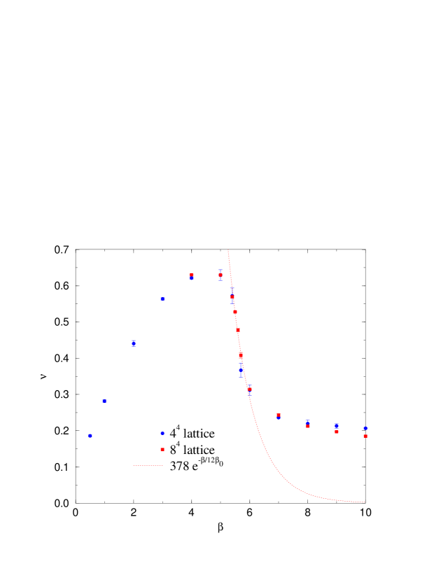
Figure 16: The Liapunov exponent $\nu$ is shown as a function of $\beta$ for pure $SU(3)$ gauge theory on $4^{4}$ and $8^{4}$ lattices. The curve is a one-parameter fit of the functional form given in eq. (7) to four of the $8^{4}$ data points ($\beta=5.4$, $5.5$, $5.6$, and $5.7$). The data was measured on three $4^{4}$ configurations and two $8^{4}$ configurations.

It is dangerous to rely too much on asymptotic scaling results obtained on such small lattices, so we will content ourselves with the statement that our data is consistent with our hypothesis that $\nu\xi$ is a constant. The value of $\nu$ is also sufficiently small that the amplification of rounding errors for trajectories of length $\tau=\xi$ is a factor of $O(1)$, and thus unimportant.

We do not have a clear understanding of why the value of $\nu$ at large $\beta$ is so large for $4^{4}$ lattices, other than the obvious suggestion that this is a finite size artefact. The data from $8^{4}$ lattices shows a small decrease in $\nu$ for large $\beta$, but this is not convincing evidence that the data will eventually fall onto our hypothetical asymptotic scaling curve.

We can gain a little more understanding of the mechanism by which $\nu$ could decrease as we approach the continuum limit by noting that $\nu$ depends on $\beta$ in two ways: there is an explicit $\beta$-dependence of the equations of motion, and there is an implicit $\beta$-dependence in the equilibrium ensemble of configurations over which $\nu$ is measured. This latter effect is illustrated in Figure 17, where we plot $\ln||\Delta\delta U||$ against $\tau$ for $\beta=5.1$ and $\kappa=0.16$ on a $4^{4}$ lattice for three different configurations, one hot, one cold, and one chosen at random from the equilibrium distribution. The hot configuration yields a larger Liapunov exponent than the equilibrium one, and the cold configuration is consistent with a power-law dependence of $||\Delta\delta U||$ on $\tau$. This result suggests that we should not expect to get the correct continuum result from lattices which are too small to be in the confined phase (even if we wanted to consider a finite temperature system in the deconfined phase we should at least ensure that the spatial volume is large enough).

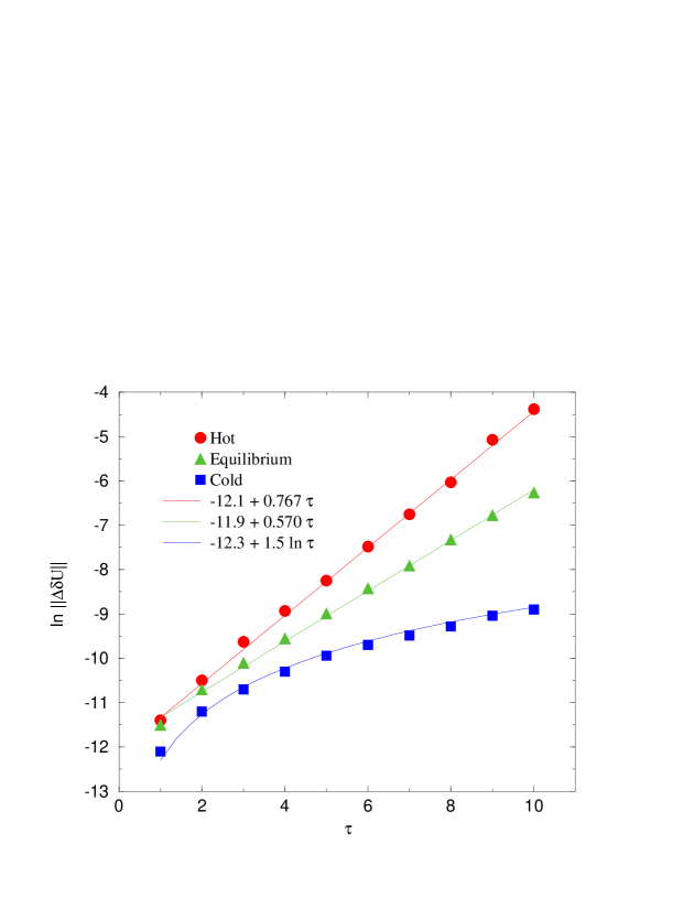
Figure 17: $\ln||\Delta\delta U||$ is shown as a function of trajectory length $\tau$ (with $\beta=5.1$, $\kappa=0.16$, and $\delta\tau=0.1$ on a $4^{4}$ lattice) for starting gauge field configurations which are “hot” (all link variables $U_{\mu}(x)$ chosen independently according to $SU(3)$ Haar measure), “equilibrium” (a typical configuration chosen from the equilibrium ensemble), and “cold” (all link variables $U_{\mu}(x)=1$). Fits of the form $||\Delta\delta U||=ke^{\nu\tau}$ for the hot and equilibrium configurations and $||\Delta\delta U||=k\tau^{3/2}$ for the cold configuration are shown.

In Figure 17 we also show two-parameter fits to the hot and equilibrium trajectories of the form $||\Delta\delta U||\propto e^{\nu\tau}$, and a one-parameter fit to the cold trajectory of the form $||\Delta\delta U||\propto\tau^{3/2}$. These fits are stable if we add more free parameters by fitting to a combination of an exponential and power dependence. The power-law behavior of the cold trajectory may be explained by a combination of a factor of $\sqrt{\tau}$ for the random walk evolution of rounding errors and a linear factor characteristic of the divergence of nearby trajectories for interacting dynamical systems in the stable (non-chaotic) region of phase space. .

7.3 Reversibility and Conjugate Gradient Accuracy

Our final topic is to investigate the effect of inaccurate CG solutions on instabilities and reversibility for dynamical fermion computations.

In Figure 18 we show the dependence of the Liapunov exponent $\nu$ and the Metropolis acceptance rate as a function of the logarithm of the CG residual for a time-symmetric (zero) initial CG vector. We define the CG residual for the approximate solution $x^{\prime}$ of the linear equations $Ax=b$ as $r\equiv||b-Ax^{\prime}||/||b||$. We also show the logarithm of the coefficient $k(r)$ for completeness.

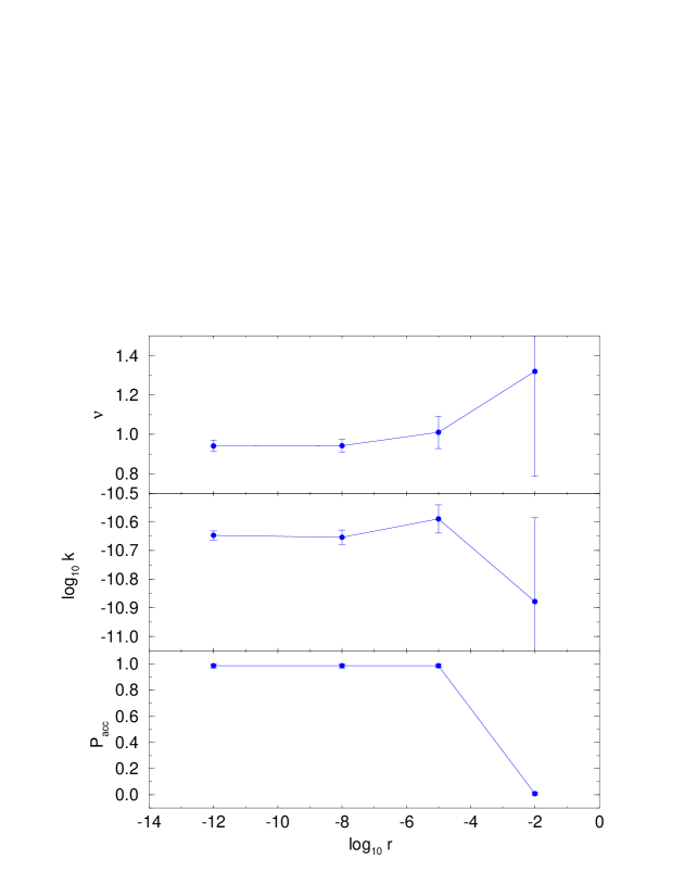
Figure 18: The dependence of $P_{\hbox{\rm\tiny acc}}$ and $||\Delta\delta U||$ on the CG residual $r$. We write $||\Delta\delta U||=ke^{\nu\tau}$, where the coefficient $k$ and exponent $\nu$ are functions of $r$. A time-symmetric zero initial CG vector was used. The data is for $4^{4}$ lattices at $\beta=3.5$ and $\kappa=0.2225$ with $\delta\tau=0.01$.

The results clearly show that the choice of residual has no effect for $r<10^{-5}$, and that for $r>10^{-2}$ the acceptance rate is essentially zero. There would seem to be no benefit from finding the solution more accurately than is needed to give a reasonable acceptance rate.

The effect of improving the convergence of the CG algorithm by using a time-asymmetric initial vector is illustrated in Figure 19. For a residual $r=10^{-8}$ the solution vector is sufficiently independent of the starting vector that the choice of initial vector has no effect on the reversibility (or otherwise) of the trajectory. On the other hand, for $r=10^{-5}$ there is a large difference between the time-symmetric start and the intrinsically irreversible time-asymmetric starts.

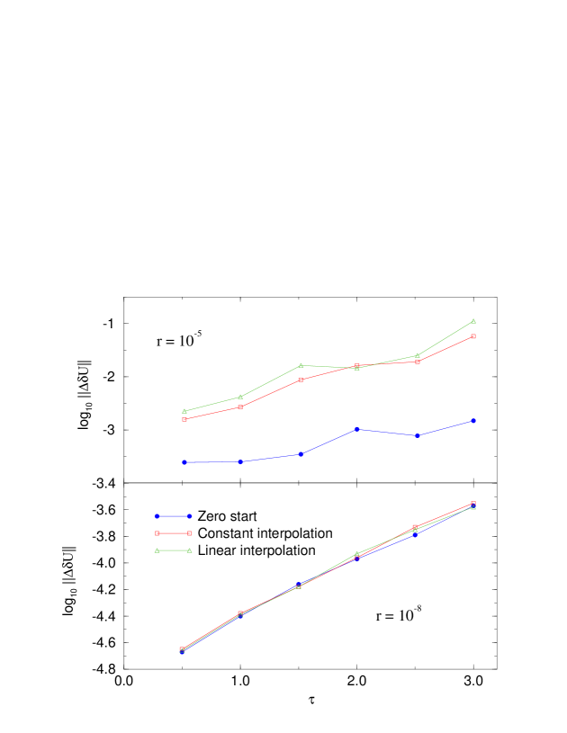
Figure 19: The dependence of $\ln||\Delta\delta U||$ on $\tau$ for different choices of initial vector for the CG algorithm. The results for the time-symmetric zero start are to be compared with those for which the initial CG vector was chosen to be the solution from the previous time step (constant interpolation), and a linear extrapolation from the previous two time steps (linear interpolation). For a residual $r=10^{-8}$ the initial vector has little effect upon the solution obtained, but for the larger residual $r=10^{-5}$ the explicit violation of reversibility is very significant. The data is from $4^{4}$ lattices with $\beta=3.5$, $\kappa=0.2225$, and $\delta\tau=0.02$.

It is clear that the reduction in the number of CG iterations required to reach a prescribed residual obtained by using an starting vector derived from previous nearby solutions [14] needs to be offset against the need to have a more accurate solution in order to avoid increased reversibility errors. To reach definitive conclusions more extensive studies would have to be done.

8 Conclusions

• Instabilities and the concomitant amplification of rounding errors caused by inaccurate numerical integration of the equations of motion should not be a problem if the integration step size is chosen suitably.

• The instabilities due to integration errors become unimportant as $V\to\infty$.

• We hypothesize that the Liapunov exponent falls as $\nu\propto\xi^{-1}$ for sufficiently large correlation lengths $\xi$, and therefore we can choose trajectories of length $\tau\propto\xi$ which may reduce critical slowing down without suffering from exponentially large amplification of rounding errors.

• The measured values of the Liapunov exponent are of $O(1)$, so the exponential amplification factor for trajectories of length $\tau\approx\xi$ are this only $e^{\nu\xi}=O(1)$.

• We have found examples with large reversibility errors but reasonable acceptance rate and small $|\Delta\delta H|$. It is always prudent to verify that $||\Delta\delta U||$ is small.

References

- [1] A. D. Kennedy. Hybrid Monte Carlo. In A. Billoire, R. Lacaze, A. Morel, O. Napoly, and J. Zinn-Justin, editors, Field Theory on the Lattice, volume B4 of Nuclear Physics (Proceedings Supplements), 1988. 1987 International Conference on Field Theory on a Lattice, Seillac, France.
- [2] Simon Duane, A. D. Kennedy, Brian J. Pendleton, and Duncan Roweth. Hybrid Monte Carlo. Phys. Lett., 195B(2):216–222, 1987.
- [3] A. D. Kennedy. The theory of Hybrid Stochastic algorithms. In P. H. Damgaard et al., editors, Probabilistic Methods in Quantum Field Theory and Quantum Gravity, pages 209–223, New York, 1990. NATO, Plenum Press. Lectures given at the workshop on “Probabilistic Methods in Quantum Field Theory and Quantum Gravity,” Cargése, August 1989.
- [4] Alan M. Horowitz. A generalized guided Monte Carlo algorithm. Phys. Lett., B268:247–252, 1991.
- [5] H. Gausterer and M. Salmhofer. Remarks on global Monte Carlo algorithms. Phys. Rev., D40(8):2723–2726, October 1989.
- [6] Sourendu Gupta, Anders Irbäck, Frithjof Karsch, and Bengt Petersson. The acceptance probability in the Hybrid Monte Carlo method. Phys. Lett., B242:437–443, 1990.
- [7] A. D. Kennedy and Brian J. Pendleton. Acceptances and autocorrelations in Hybrid Monte Carlo. In Urs M. Heller, A. D. Kennedy, and Sergiu Sanielevici, editors, Lattice ’90, volume B20 of Nuclear Physics (Proceedings Supplements), pages 118–121, 1991. Talk presented at “Lattice ’90,” Tallahassee.
- [8] A. D. Kennedy and Brian J. Pendleton. Some exact results for Hybrid Monte Carlo. In preparation, 1996.
- [9] A. D. Kennedy, Robert G. Edwards, Hidetoshi Mino, and Brian J. Pendleton. Tuning the generalized Hybrid Monte Carlo algorithm. In Tien D. Kieu, Bruce H. J. McKellar, and Anthony J. Guttmann, editors, Lattice ’95, volume B47 of Nuclear Physics (Proceedings Supplements), pages 781–784, 1995. Proceedings of the 13th International Symposium on Lattice Field Theory, Melbourne, Australia, 11–15 July 1995.
- [10] Khalil M. Bitar, Robert G. Edwards, Urs M. Heller, and A. D. Kennedy. On the dynamics of light quarks in QCD. In Jan Smit and Pierre van Baal, editors, Lattice ’92, volume B30 of Nuclear Physics (Proceedings Supplements), pages 249–252, March 1993. Proceedings of the International Symposium on Lattice Field Theory, Amsterdam, the Netherlands, 15–19 September 1992.
- [11] Karl Jansen and Chuan Liu. Kramer’s equation algorithm for simulations of QCD with two flavors of Wilson fermions and gauge group . Nucl. Phys., B453:375–394, 1995.
- [12] Karl Jansen and Chuan Liu. Liapunov exponents and the reversibility of molecular dynamics algorithms. Preprint, DESY, 1996.
- [13] Holger B. Nielsen, H. H. Rugh, and S. E. Rugh. Chaos and scaling in classical non-abelian gauge fields. Chao–dyn/9605013, Niels Bohr Institute, May 1996.
- [14] Richard C. Brower, T. Ivanenko, A. R. Levi, and K. N. Orginos. Chronological inversion method for the dirac matrix in Hybrid Monte Carlo. Preprint, Boston University, 1995.