Spectral functions at small energies and the electrical conductivity
in hot, quenched lattice QCD

Abstract

In lattice QCD, the Maximum Entropy Method can be used to reconstruct spectral functions from euclidean correlators obtained in numerical simulations. We show that at finite temperature the most commonly used algorithm, employing Bryan’s method, is inherently unstable at small energies and give a modification that avoids this. We demonstrate this approach using the vector current-current correlator obtained in quenched QCD at finite temperature. Our first results indicate a small electrical conductivity above the deconfinement transition.

In the deconfined, high-temperature phase of Quantum Chromodynamics, the behaviour of spectral functions of conserved currents at small energies is of intrinsic interest due to its relation with transport properties of the quark-gluon plasma (QGP). According to the Kubo formulas Kadanoff , transport coefficients, such as the shear and bulk viscosities and the electrical conductivity, are proportional to the slope of appropriate spectral functions at vanishing energy. The success of e.g. ideal hydrodynamics in heavy ion phenomenology, assuming vanishing viscosities and requiring early thermalization Heinz:2001xi , has lead to the notion Gyulassy:2004vg that the QGP created in relativistic heavy ion collisions at RHIC is strongly coupled and that the ratio of shear viscosity to entropy density in this sQGP may be close to the conjectured lower bound Kovtun:2004de reached in thermal field theories that admit a gravity dual Policastro:2001yc .

In order to put these ideas on firm footing, it is important to have a first-principle calculation of transport coefficients in the strongly coupled regime of hot QCD. As is well known Karsch:1986cq ; Aarts:2002cc , a nonperturbative calculation using lattice QCD is difficult due to the necessity to perform an analytic continuation from imaginary to real time. The most common approach used to obtain spectral functions from euclidean correlators is the Maximum Entropy Method Asakawa:2000tr , employing Bryan’s algorithm Bryan . Our first aim in this Letter is to discuss this method in some detail and point out a source of numerical instabilities present in most finite-temperature studies available to date. We show how the algorithm can be modified to avoid this problem. Our second aim is to apply the new method to the vector current-current correlator, obtained in quenched lattice QCD simulations at finite temperature, using staggered quarks. We study the behaviour at small energies and argue that it allows us to extract a value for electrical conductivity in the strongly coupled regime above the deconfinement transition.

Maximum Entropy Method – The relation between the euclidean correlator $G(\tau)=\int d^{3}x\,\langle J(\tau,{\mathbf{x}})J^{\dagger}(0,{\mathbf{0}})\rangle$ at zero momentum and the corresponding spectral function $\rho(\omega)$ reads

$$G(\tau)=\int_{0}^{\infty}\frac{d\omega}{2\pi}\,K(\omega,\tau)\rho(\omega),$$ (1)

where the kernel is given by

$$K(\omega,\tau)=\frac{\cosh[\omega(\tau-1/2T)]}{\sinh(\omega/2T)}.$$ (2)

We consider (local) meson operators of the form $J(\tau,{\mathbf{x}})=\bar{q}(\tau,{\mathbf{x}})\Gamma q(\tau,{\mathbf{x}})$, where $\Gamma$ depends on the channel under consideration. The temperature $T$ is related to the euclidean temporal extent $N_{\tau}$ by $1/T=aN_{\tau}$, where $a$ is the (temporal) lattice spacing. The difficulty in inverting relation (1) is due to the fact that $G(\tau)$ is obtained numerically at a discrete set of points $\tau_{i}=\tau_{\rm min}+(i-1)a$ ($i=1,\ldots,N$), where the number of data points $N$ is typically ${\cal O}(10)$, whereas $\rho(\omega)$ is in principle a continuous function of $\omega$. Simple properties of the kernel and spectral functions allow us to cutoff the $\omega$ integral at $\omega_{\rm max}$. The resulting finite interval is discretized as $\omega_{n}=n\Delta\omega$ ($n=1,\ldots,N_{\omega}$), where $N_{\omega}$ is typically ${\cal O}(10^{3})$, making a simple inversion ill-defined (below we suppress the index $n$ in $\omega_{n}$ where possible).

Using the ideas of Bayesian probability theory, one may construct the most probable spectral function by maximizing the conditional probability $P[\rho|DH]$, where $D$ indicates the data and $H$ some additional prior knowledge. In the Maximum Entropy Method (MEM), the prior knowledge is encoded in an entropy term,

$$S=\int_{0}^{\infty}\frac{d\omega}{2\pi}\left[\rho(\omega)-m(\omega)-\rho(\omega)\ln\frac{\rho(\omega)}{m(\omega)}\right],$$ (3)

where $m(\omega)$ is the so-called default model, containing the additional information. An often used default model is $m(\omega)=m_{0}\omega^{2}$, with $m_{0}$ a (channel-dependent) constant. This choice is motivated by the large-$\omega$ behaviour of meson spectral functions in the continuum theory, which is accessible in perturbation theory. The conditional probability to be extremized reads

$$P[\rho|DH]=\exp\left(-\frac{1}{2}\chi^{2}+\alpha S\right),$$ (4)

where $\chi^{2}$ is the standard likelihood function and $\alpha$ is a parameter balancing the relative importance of the data and the prior knowledge. Since $\rho(\omega)$ is nonnegative for positive $\omega$, it is written as

$$\rho(\omega)=m(\omega)\exp f(\omega),$$ (5)

where $f(\omega)$ is to be determined.

Bryan’s approach – To make the problem well-defined, the arbitrary function $f(\omega)$ has to be reduced to one containing at most $N$ parameters, i.e. it has to be restricted to an $N$ dimensional subspace. In Bryan’s algorithm the subspace is determined using a singular value decomposition (SVD). After discretizing the $\omega$ integral, the kernel $K(\omega_{n},\tau_{i})$ is viewed as a $N_{\omega}\times N$ matrix. The SVD theorem states that it can be written as $K=UWV^{T}$, with $U$ an $N_{\omega}\times N$ matrix satisfying $U^{T}U=1\!\!1_{N\times N}$, $W=\mbox{diag}(w_{1},\dots,w_{N})$ with $w_{1}\geq\ldots\geq w_{N}\geq 0$, and $V$ an $N\times N$ matrix satisfying $VV^{T}=V^{T}V=1\!\!1_{N\times N}$. The dimension $N_{s}$ of the subspace is determined by the singular values $w_{i}$. Due to the reflection symmetry $K(\omega,1/T-\tau)=K(\omega,\tau)$, one finds that $N_{s}\leq N\leq N_{\tau}/2+1$. Discarding the contact term at $\tau=0$, we use below the maximal range $N_{s}=N=N_{\tau}/2$, such that all data points at $1\leq\tau_{i}/a\leq N_{\tau}/2$ are included. In Bryan’s algorithm the subspace is defined as the space spanned by the column vectors of $U$, i.e. the $N$ vectors $u_{i}$ ($i=1,\ldots,N$) with elements $u_{i}(\omega_{n})=U_{ni}$. Since $U$ is orthogonal, these vectors are linearly independent and normalized, with the inner product $\langle u_{i}|u_{j}\rangle\equiv\sum_{n=1}^{N_{\omega}}u_{i}(\omega_{n})u_{j}(\omega_{n})=\delta_{ij}$. It follows from the extremum condition that $f(\omega)$ can be parametrized as

$$f(\omega)=\sum_{i=1}^{N}c_{i}u_{i}(\omega).$$ (6)

This reduces the problem to the determination of $N$ coefficients $c_{i}$, as desired.

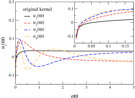
Figure 1: First four basis functions $u_{i}(\omega)$ as a function of $a\omega$ for $a\omega_{\rm max}=5$, $N_{\omega}=1000$, $N_{\tau}=24$, using the standard kernel. The inset shows a blow-up of the small energy region.

The $u_{i}$ functions should therefore be regarded as basis functions and it is interesting to study how they behave. In Fig. 1 we show the first four basis functions determined using the SVD of $K(\omega_{n},\tau_{i})$ for the case that $N_{\omega}=1000$ and $N=N_{\tau}/2=12$. The cutoff is $a\omega_{\rm max}=5$. Details of the basis functions depend on the choice of $N_{\omega}$ and $N$, but we find that the $i$’th function crosses zero $i$ times. The inset shows a blowup of the small energy behaviour. It can be seen that all basis functions seem to diverge in the small energy limit (although they are still normalizable). This is because the kernel itself diverges for small $\omega$, since

$$\lim_{\omega\to 0}K(\omega,\tau)=\frac{2T}{\omega}+\frac{\omega}{T}\left[\frac{1}{6}-\tau T(1-\tau T)\right]+{\cal O}\left(\frac{\omega^{3}}{T^{3}}\right).$$ (7)

Due to this divergence, it is not possible to include the point at $\omega=0$ (note that the limits $T\to 0$ and $\omega\to 0$ do not commute).

In the MEM analysis of lattice correlators at finite temperature, it is often found (see e.g. Ref. Aarts:2006cq and references therein) that the small energy behaviour is unstable: the value of the spectral function at the smallest nonzero $\omega$ value is inconsistent with values at larger energies and the $\omega\to 0$ behaviour depends on $\Delta\omega$, indicating that it is an artefact of the method. Moreover MEM does not always converge. Unstable features in the algorithm at small energies prevent of course insight in transport properties of the QGP.

Modification of Bryan’s algorithm – As indicated above, the divergence of the kernel at small energies can lead to a numerically unstable algorithm. Fortunately, this can easily be avoided by writing

$$\overline{K}(\omega,\tau)=\frac{\omega}{2T}K(\omega,\tau),\;\;\;\;\;\;\;\;\overline{\rho}(\omega)=\frac{2T}{\omega}\rho(\omega),$$ (8)

such that $K(\omega,\tau)\rho(\omega)=\overline{K}(\omega,\tau)\overline{\rho}(\omega)$. We may now repeat the SVD for $\overline{K}(\omega_{n},\tau_{i})$. We find that both kernels give the same identification of the dimension of the subspace. The first four new basis functions $\overline{u}_{i}$ are shown in Fig. 2. The inset shows again a blow-up. Since $\overline{K}(0,\tau)=1$, the basis functions take a finite value at small $\omega$ and $\overline{u}_{i}(0)$ is well-defined for all $i$. From now on we include the point at $\omega=0$ in the analysis. The redefined spectral function is parametrized as

$$\overline{\rho}(\omega)=\overline{m}(\omega)\exp\sum_{i=1}^{N}\overline{c}_{i}\overline{u}_{i}(\omega),$$ (9)

with the default model $\overline{m}(\omega)\sim m(\omega)/\omega$. In order to make contact with previous results, $\overline{m}(\omega)\sim\omega$ at large $\omega$. For small $\omega$, we note that we reconstruct $\overline{\rho}\sim\rho/\omega$, such that the intercept at $\omega=0$ is proportional to the appropriate transport coefficient. Specifically, for the electrical conductivity we find that

$$\frac{\sigma}{T}=\lim_{\omega\to 0}\,\frac{\rho(\omega)}{6\omega T}=\frac{\overline{\rho}(0)}{12T^{2}},$$ (10)

where in this case $\rho$ is in the vector channel ($\Gamma=\gamma_{k}$, summed over $k=1,2,3$). To allow for a nonzero intercept, we find from Eq. (9) that $\overline{m}(0)$ should be finite and nonzero. We use therefore the following default model

$$a^{2}\overline{m}(\omega)=\overline{m}_{0}(b+a\omega),$$ (11)

where $b\lesssim 1$ is a parameter that can be varied to assess the default-model dependence of spectral functions in the low-energy regime.

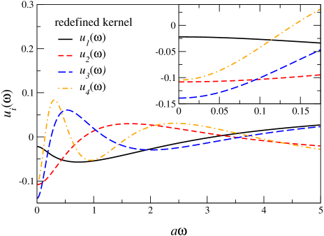
Figure 2: As in Fig. 1, using the redefined kernel $\overline{K}(\omega,\tau)$.

	$\beta$	$a^{-1}$ (GeV)	$N_{\sigma}^{3}\times N_{\tau}$	$T/T_{c}$	# conf
cold	6.5	4.04	$48^{3}\times 24$	0.62	100
hot	7.192	9.72	$64^{3}\times 24$	1.5	100
very hot	7.192	9.72	$64^{3}\times 16$	2.25	50

Table 1: Lattice parameters. Estimates for the lattice spacing and temperature are taken from Ref. Datta:2003ww .

Lattice QCD – We now apply the modified algorithm to the euclidean correlator in the vector channel, obtained in quenched lattice QCD simulations at finite temperature. Lattice details are given in Table 1. The two lattices above $T_{c}$ differ only in temperature, while the lattice below $T_{c}$ is coarser but has $N_{\tau}=24$, in common with the hot one. We use light staggered quarks with a bare mass of $am=0.01$. As is well known, the pure gauge action has a global $Z_{3}$ symmetry, which is broken by the presence of fermions in full QCD. To incorporate this, we multiply the link variables by an element of $Z_{3}$ in the calculation of the quark propagators so that the phase of the Polyakov loop is approximately real. Chiral symmetry restoration at $T>T_{c}$ is then clearly visible: the pseudoscalar and scalar correlators coincide Aarts:2006cq .

For staggered fermions the MEM analysis is complicated due to the mixing of two signals in the correlator. The equivalent of relation (1) reads

$$G^{\rm stag}(\tau)=\int_{0}^{\infty}\frac{d\omega}{2\pi}\,K(\tau,\omega)\left[\rho(\omega)-(-1)^{\tau/a}\tilde{\rho}(\omega)\right],$$ (12)

where $\tilde{\rho}$ is related to $\rho$ by changing $\Gamma$ to $\tilde{\Gamma}=\gamma_{4}\gamma_{5}\Gamma$. In practice we perform an independent MEM analysis on the even and odd time slices, obtaining $\rho_{\rm even}=\rho-\tilde{\rho}$ and $\rho_{\rm odd}=\rho+\tilde{\rho}$ and combine these to get $\rho$. Let us remark here that while the original formulation, using $K(\omega,\tau)$, failed to converge in some cases, we found that the new method worked successfully (we have studied the vector and pseudoscalar channels inprep ). In cases where both methods worked we found comparable results for spectral functions in most of the energy range but deviations in the low-energy region, as expected.

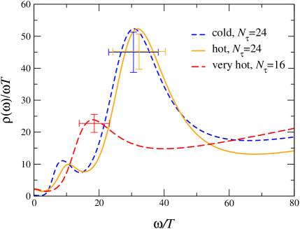
Figure 3: Vector spectral functions $\rho(\omega)/\omega T$ as a function of $\omega/T$. We used $N_{\omega}=1000$, $a\omega_{\rm max}=5$, $b=1$.

In Fig. 3 we show the vector spectral functions $\rho(\omega)$ normalized by $\omega T$ as a function of $\omega/T$ for the three temperatures. Our treatment of $\alpha$ follows Ref. Asakawa:2000tr . The large $\omega$ behaviour at $a\omega\gtrsim 3$ is determined by the continuum default model, $\rho(\omega)/\omega\sim m_{0}\omega$ (recall that $\omega/T=N_{\tau}a\omega$). In most MEM studies we carried out we find “bumps” at $1\lesssim a\omega\lesssim 2$: within uncertainties these do not depend on the channel under consideration, quark mass or external momentum Aarts:2006cq ; inprep . We interpret them as lattice artefacts present due to the difference between continuum and lattice fermion dispersion relation (see Ref. Aarts:2005hg for an analysis of free staggered quarks). The peak structure at $\omega/T\sim 9$ on the cold lattice is the rho-meson, which is more clearly visible in plots of $\rho(\omega)/\omega^{2}$ vs. $\omega/T$ Aarts:2006cq . The rho-peak is less pronounced on the hot lattice and seems to have vanished on the very hot lattice. Error bars are explained in Ref. Asakawa:2000tr .

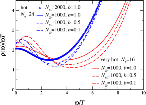
Figure 4: Default model dependence of $\rho(\omega)/\omega T$ for $N_{\tau}=24$ (hot) and $16$ (very hot) in the low-energy region. We show results for $N_{\omega}=1000,2000$ and $b=1.0,0.5,0.1$ at fixed $a\omega_{\rm max}=5$.

Above $T_{c}$ a nonzero intercept at $\omega=0$ can be seen. In the cold phase the intercept is an order of magnitude smaller. A blow-up of $\rho(\omega)/\omega T$ is shown in Fig. 4. In the high-temperature weakly-coupled theory, the transport contribution is located at $\omega/T\sim g^{4}(T)\ll 1$, where the spectral function behaves as $\rho(\omega)/\omega T\sim 1/g^{4}(T)\gg 1$. As a result the euclidean correlator is insensitive to the details of the spectral function Aarts:2002cc . Here, by contrast, we find a clear signal for nonzero spectral weight varying smoothly in the range $0\lesssim\omega/T\lesssim 4$. To assess this, we have varied $N_{\omega}$, $a\omega_{\rm max}$ and the parameter $b$ in Eq. (11). In the case that we take $b=0$ (therefore disallowing a nonzero intercept), we find that the MEM routine does not converge. Results with $N_{\omega}=2000$ cannot be distinguished from those obtained with $N_{\omega}=1000$. These findings suggest that nonzero spectral weight and a finite intercept are robust outcomes. Dividing the intercept at $\omega=0$ by 6 yields the electrical conductivity. We find $\sigma/T=0.4\pm 0.1$, where the error is an indication of the uncertainty in the MEM reconstruction Gupta:2003zh . Statistical uncertainty and the effect of operator normalization Daniel:1987aa are expected to be smaller.

Outlook – We identified a source for numerical instabilities in the standard formulation of MEM with Bryan’s approach at finite temperature and showed how this can be avoided. We then applied this new method to the vector current-current correlator obtained in quenched lattice QCD at finite temperature. We found a robust signal for a small but nonzero value of the electrical conductivity above the deconfinement transition, in line with the notion of the sQGP. Directions for the future are many. It is important to repeat the analysis using Wilson fermions and the conserved point split current, and to include the shear and bulk viscosity as well. The effect of dynamical quarks can be investigated in two-flavour QCD on highly anisotropic lattices Aarts:2007pk . We emphasize once more that the new formulation is essential for analyzing the low-energy region.

- (1) See e.g. L. P. Kadanoff and P. C. Martin, Ann. Phys. 24, 419 (1963).
- (2) U. W. Heinz and P. F. Kolb, Nucl. Phys. A 702 (2002) 269.
- (3) M. Gyulassy, nucl-th/0403032; M. Gyulassy and L. McLerran, Nucl. Phys. A 750 (2005) 30; E. V. Shuryak, Nucl. Phys. A 750 (2005) 64.
- (4) P. Kovtun, D. T. Son and A. O. Starinets, Phys. Rev. Lett. 94 (2005) 111601.
- (5) G. Policastro, D. T. Son and A. O. Starinets, Phys. Rev. Lett. 87 (2001) 081601; A. Buchel and J. T. Liu, Phys. Rev. Lett. 93 (2004) 090602.
- (6) F. Karsch and H. W. Wyld, Phys. Rev. D 35 (1987) 2518.
- (7) G. Aarts and J. M. Martínez Resco, JHEP 0204 (2002) 053; Nucl. Phys. Proc. Suppl. 119 (2003) 505.
- (8) For a review in the context of lattice QCD, see M. Asakawa, T. Hatsuda and Y. Nakahara, Prog. Part. Nucl. Phys. 46, 459 (2001).
- (9) R.K. Bryan, Eur. Biophys. J. 18 (1990) 165.
- (10) S. Datta, F. Karsch, P. Petreczky and I. Wetzorke, Phys. Rev. D 69, 094507 (2004).
- (11) G. Aarts and J. M. Martínez Resco, Nucl. Phys. B 726 (2005) 93.
- (12) G. Aarts, C. Allton, J. Foley, S. Hands and S. Kim, PoS LAT2006 (2006) 134 [hep-lat/0610061].
- (13) G. Aarts, C. Allton, J. Foley, S. Hands and S. Kim, in preparation.
- (14) For an earlier calculation of the electrical conductivity in lattice QCD, see S. Gupta, Phys. Lett. B 597, 57 (2004).
- (15) D. Daniel and S. N. Sheard, Nucl. Phys. B 302 (1988) 471.
- (16) G. Aarts et al., arXiv:0705.2198 [hep-lat]; PoS LAT2006 (2006) 126; R. Morrin et al., PoS LAT2005 (2006) 176.
- (17) A. Jakovac, P. Petreczky, K. Petrov and A. Velytsky, Phys. Rev. D 75 (2007) 014506.