Confining String and Its Widening in ${\mathrm{HP}^{1}}$ Embedding Approach

Abstract

Structure of confining string in terms of the topological charge density and the action density is studied in $SU(2)$ Yang-Mills theory on the lattice using ${\mathrm{HP}^{1}}$ $\sigma$-model embedding approach. We find that the confining flux tube noticeably suppresses both the topological charge and the action densities. Beyond the string formation length the string cross section in terms of these quantities is well described by a Gaussian profile. In both cases the squared string width is found to be a logarithmic function of the string length confirming the Lüscher widening of the chromoelectric string. Characteristic string scales in terms of the topological and action densities are estimated as well.

I Introduction

It is commonly believed that the phenomenon of the quark confinement in QCD happens due to formation of the chromoelectric string spanned between quark and anti-quark. In fact, various numerical simulations in QCD both in quenched and in unquenched limits indicate that in the QCD vacuum the fundamental color charges (quarks) are connected by a string-like structure Bali:1994de (see, e.g., Ref Bali:review and references therein), which can be seen directly in gluonic energy and action density ref:string:energy-action ; Bissey as well as in other related quantities ref:string:other . Physically, the string is formed by squeezed fluxes of chromoelectric fields coming out of quarks. The chromoelectric string possesses a non-zero tension providing steady attracting force which makes the quarks confined into colorless hadrons.

There are various effects caused by the strong chromoelectric fields of the QCD string. Besides the enhancement of the gluonic energy density, the string is characterized by the suppression of the gluonic action density ref:sum-rules , as well as by the suppression Chernodub:2005gz of the ${\langle A^{2}\rangle}$-condensate ref:A2 . Some features of the QCD string are consistent with the dual superconductor model of the color confinement ref:dual:superconductor which attributes the color flux squeezing to a (dual) Meissner effect originating from condensation of particular (“monopole-like”) gluon field configurations ref:reviews . Naturally, chromoelectric string formation has a great impact on both gluons and quarks, however, in latter case the confinement of color manifests itself in yet another way. There are numerical indications that the chiral symmetry, originally broken by non-perturbative effects in the low temperature QCD, is (partially) restored inside the string ref:Laermann . The effect is revealed by local suppression of the chiral condensate $\langle\bar{\psi}\psi\rangle$ in the vicinity of the string. The same effect is also observed numerically in the neighborhood of individual heavy quarks ref:chiral:quark , indicating that the strong chromoelectric fields tend to restore the chiral symmetry. Since the chiral properties of the vacuum are tightly related to its topology, one expects generically that strong chromoelectric field of the string severely affects the topological charge density. Indeed, the anti-correlation between the QCD string and the topological charge density was discovered in numerical simulation of Ref. string:topcharge:first in the so called “cooled” $SU(3)$ vacuum. The investigation was developed further in Ref. string:topcharge with the help of the same cooling method which is a gradual transformation of the quantum (“hot”) fields towards the classical (“cold”) vacuum. The cooling is aimed to reduce the topologically trivial effects of divergent zero-point fluctuations. This important result – obtained with the simplest lattice definitions of the topological charge – is a first numerical indication that the QCD string suppresses topological fluctuations. In this paper we investigate, in particular, the structure of confining string in terms of the topological charge density. The problem is conceptually and technically challenging and therefore it calls for a few physically motivated simplifications. First, we refrain from using the cooling approach because it certainly wipes out local topology of the real (uncooled) vacuum. Indeed, the fluctuations of the topological charge inside the chromoelectric string were found to depend crucially upon the cooling parameters string:topcharge:first ; string:topcharge and therefore are affected by uncontrollable systematic errors. Other essential simplifications used in this paper are as follows:

Quenched vacuum. For our purposes it is natural to consider quenched approximation because dynamical quarks screen the test color charges and break the string. As a result the correlation between the string and any locally defined quantity disappears at sufficiently large separations between the test charges. Thus the choice of the quenched vacuum is crucial, as it allows to discriminate between the string breaking and the actual correlation effects.

Reduced number of colors. It is advantageous to utilize the known similarity between the $SU(2)$ and $SU(3)$ gauge models. Since nonperturbative aspects are alike in these theories, we naturally expect that the behavior of the topological charge density around the string in the realistic $SU(3)$ case is qualitatively the same as for the $SU(2)$ gauge group studied in our paper. Apart from the obvious computational simplifications, restriction to $SU(2)$ gauge theory allows us to address unambiguously the next urgent problem of

Ultraviolet (UV) fluctuations. Indeed, simply on dimensional grounds one expects that the vacuum topological density is power-like divergent ${\langle q^{2}\rangle}\sim 1/a^{8}$, $a$ being the lattice spacing (the inverse UV cutoff). However, the leading UV divergence should not be sensitive to the quark-antiquark separation. Note that this is not so in the case of subleading power corrections, which depend also upon the infrared (IR) scale (denoted $\Lambda_{QCD}$ generically). Therefore in order to study the correlation of the string and the topological density it would be advantageous to remove the leading (and only leading) power divergence in ${\langle q^{2}\rangle}$ since it gives identically vanishing but otherwise numerically destructive contribution to the correlation function.

In view of the above points the choice of the topological density operator, which is free from additional parameters, becomes, in fact, almost unique. Indeed, the cooling approach was rejected for reasons explained above. As far as the fermionic definition overlap is concerned, in the numerical implementations it is either not parameter free or is not capable to filter out exclusively the leading power divergence. Indeed, the essence of the construction is to sum up the individual contributions of eigenmodes of overlap Dirac operator, ranked with corresponding eigenvalues. It is known Horvath:2005cv that the full tower of eigenmodes indeed reproduces $\sim 1/a^{8}$ behavior, while the restriction to lowest eigenvalues Horvath:2003yj introduces explicit and a priori ambiguous cut on the leading singularity. Therefore the essentially unique alternative construction which fits the above requirements is ${\mathrm{HP}^{1}}$ $\sigma$-model embedding approach Gubarev:2005rs ; Boyko:2006jt which is to be reviewed in Section  II. Here we only mention that this method indeed provides parameter free definition of the topological density in which the leading power divergence is removed. Note that the removal of leading perturbative contributions from various observables in ${\mathrm{HP}^{1}}$ embedding approach had not been proved rigorously, however, in all examples considered so far it turns out to be the case. Moreover, the subleading power corrections seem to be left intact by the corresponding gauge covariant ${\mathrm{HP}^{1}}$-projection procedure. What is even more important is that near the continuum limit the ${\mathrm{HP}^{1}}$-projected fields capture the majority of non-perturbative aspects of $SU(2)$ Yang-Mills theory and reproduce, for instance, the full tension of the confining string and (quenched) quark condensate (see Refs. Gubarev:2005rs ; Boyko:2006jt for further details). Being numerically superior, the ${\mathrm{HP}^{1}}$ embedding approach is naturally our method of choice to investigate the topological aspects of the confining string and to study its geometrical properties. For discussion of other methods which allow to “filter out” topological properties of the vacuum out of the ultraviolet noise see Ref. ref:other:methods .

However, the advantages of our method are not coming for free, the price is the intrinsic non-locality: the ${\mathrm{HP}^{1}}$ $\sigma$-model fields constructed from given $SU(2)$ gauge background are not local in terms of the original gauge potentials. However the characteristic range of non-locality is certainly less than $\lesssim 0.3~{}\mathrm{fm}$ and is comparable with the expected Bali:1994de half-width of the flux tube as it is determined by the string action density profile. We conclude therefore that the non-locality of our method should not be essential for large enough quark-antiquark separations.

The knowledge of the string profiles immediately reveals an important feature of the chromoelectric string known as the string widening. This rather general phenomenon occurs in various gauge and spin systems possessing the string-like excitations. As it was predicted by Lüscher Luscher:1980iy , quantum fluctuations force the string to fluctuate transversely in such a way that its geometrical center follows the Gaussian distribution. The squared width of the Gaussian distribution (string width) is expected to be the logarithmic function of the string length, $\delta^{2}(R)\propto\ln R$, which in quenched QCD is the distance between heavy quark-antiquark pair.

The logarithmic widening of the string was accurately seen Caselle:1995fh in the $Z\!\!\!Z_{2}$ gauge model in $(2+1)$ dimensions, and the signatures of the widening are reflected in the form of the potential between test sources connected by the string Panero:String:Effects . For other gauge theories the results are still inconclusive. For instance, the data for the string in gluodynamics width obtained via the energy density profiles Bali:1994de is consistent both with the constant behavior, $\delta(R)\approx{\mathrm{const}}$, and with the logarithmic scaling for $R\gtrsim 1\,\mbox{fm}$.

In the numerical simulations the string profile is usually overshadowed by the ultraviolet noise, which may be reduced within the certain models of the vacuum structure. For instance, the dual superconductor scenario of quark confinement ref:dual:superconductor suggests that the confining string formation is governed by the dynamics of Abelian fields calculated in a certain Abelian gauge. While this approach consistently describes particular features of the chromoelectric string, the string width is found to be length-independent both in quenched Bali:review and full Bornyakov:2003vx QCD, thus contradicting the logarithmic scaling law. Another popular approach center:confinement assumes that basic non-perturbative properties of gluons are encoded in the center degrees of freedom, the corresponding string profile was calculated in Ref. Bornyakov:2003gn . It was found that the string width itself (not its square) is a logarithmic function of the quark-antiquark distance, again contradicting the Lüscher law. Therefore the results available in the literature indicate that neither Abelian nor center degrees of freedom preserve the transverse non-perturbative fluctuations of the confining string, while the simulations within the full theory give inconclusive results. In this paper we investigate the string broadening using ${\mathrm{HP}^{1}}$-projected fields, which allow us to obtain a clean picture of the confining string both in terms of the topological density and in terms of the gluonic action distribution.

The structure of the paper is as follows. The essentials of ${\mathrm{HP}^{1}}$ $\sigma$-model embedding approach are reviewed in Sections II, while in Section III we discuss the relevant observables and theoretical expectations. In Section IV we describe the technical details of our measurements. Then the profiles of the QCD string in terms of the topological and ${\mathrm{HP}^{1}}$-projected action densities are presented in Sections V,VI, respectively, where we also discuss the degree of the string broadening at various quark-antiquark separations. Section VII is devoted to the discussion of our results.

II Review of ${\mathrm{HP}^{1}}$ embedding

In this Section we briefly review the ${\mathrm{HP}^{N}}$ $\sigma$-model embedding approach using continuum notation, for precise lattice definitions and further details see Refs. Gubarev:2005rs ; Boyko:2006jt . The most straightforward way to introduce the idea of the method is to consider first Yang-Mills theory with gauge group $SU(2)$ (group of unit quaternions) in the limit, in which the gauge potentials $A_{\mu}$ are smooth functions of space-time coordinates. Then it is known theorem (see, e.g., Ref. theorem:review for extended discussions) that $A_{\mu}$ can be represented as

$$A_{\mu}=\langle\,q\,|\partial_{\mu}|\,q\,\rangle=\sum_{i=0}^{N}\bar{q}_{i}\partial_{\mu}q_{i}\,,$$ (1)

where $|\,q\,\rangle$ is $(N+1)\times 1$ normalized $\langle\,q\,|\,q\,\rangle=1$ column vector with quaternion valued entries $q_{i}$, bar denotes quaternionic conjugation and $N$ is finite integer number, the upper bound on which is unimportant for the present discussion. Gauge covariance of (1) implies that $|\,q\,\rangle=[q_{0},...,q_{N}]^{T}$ and $|\,q\,\rangle v=[q_{0}v,...,q_{N}v]^{T}$, where $v$ is unit quaternion, $\bar{v}v=1$, are physically equivalent and therefore the set of gauge inequivalent fields $|\,q\,\rangle$ describe the quaternionic projective space ${\mathrm{HP}^{N}}$, convenient parametrization of which is provided by gauge invariant $(N+1)\times(N+1)$ projection matrices $P=|\,q\,\rangle\langle\,q\,|$. Therefore in the limit of smooth fields the $SU(2)$ Yang-Mills theory could be reformulated in terms of the non-linear $\sigma$-model with target space ${\mathrm{HP}^{N}}$. Note that in the particular case $N=1$ target space geometry simplifies greatly, ${\mathrm{HP}^{1}}=S^{4}$, and one has

$$P=|\,q\,\rangle\langle\,q\,|=\frac{1}{2}(1+\gamma^{A}n^{A})\,,\quad A=1,...,5\,,$$ (2)

where $n^{A}$ is unit five-dimensional vector and $\gamma^{A}$ are the conventional Dirac matrices. We use the same symbol $q$ to denote both the quaternions and the topological charge density. We do not expect a confusion with notation since the quaternions are used only in this Section and they are always associated with the bra-ket symbols.

The essence of ${\mathrm{HP}^{N}}$ $\sigma$-model embedding approach is to consider Eq. (1) within the Euclidean formulation of quantum $SU(2)$ Yang-Mills theory and to quantify its approximate validity for given gauge background. Namely, for any fixed gauge configuration $A_{\mu}$ one finds the “nearest” ${\mathrm{HP}^{N}}$ $\sigma$-model fields $\{|\,q_{x}\,\rangle\}$, which minimize the functional norm

$$||A-\langle\,q\,|\partial|\,q\,\rangle||\equiv F(A,|\,q\,\rangle)<F(A,|\,q^{\prime}\,\rangle)\,,$$ (3)

$$\forall\,\,\{|\,q_{x}^{\prime}\,\rangle\}\neq\{|\,q_{x}\,\rangle\}\,.$$

In fact, the problem (3) is well suited for the lattice studies and it turns out that the minimizing configuration $\{|\,q_{x}\,\rangle\}$ is essentially unique, at least for the gauge potentials numerically generated on the lattice near the continuum limit. Note that the only free parameter at this stage is the rank $N$ of the $\sigma$-model considered. Naively, one could expect that the quality of approximation $A\approx\langle\,q\,|\partial|\,q\,\rangle$ quantified by $F(A,|\,q\,\rangle)$ varies strongly with $N$, however, this turns out not to be the case. To the contrary, the functional distance $F(A,|\,q\,\rangle)$ appears to be independent on the $\sigma$-model rank and hence there are no practical reasons to go beyond the simplest $N=1$ case. In turn the restriction to $N=1$ allows to give natural and computationally superior definition of the topological charge density, which undoubtedly integrates to an integer number.

At this point it is natural to introduce the notion of ${\mathrm{HP}^{1}}$-projection. Namely, one could replace the original potentials with corresponding $\sigma$-model induced gauge connection

$$A_{\mu}~{}\to~{}A^{\mathrm{HP}}_{\mu}\equiv\langle\,q\,|\partial_{\mu}|\,q\,\rangle\,,$$ (4)

and then compare the physical content of the original and projected configurations. It turns out that $A^{\mathrm{HP}}_{\mu}$ fields are extremely weak, the corresponding curvature is by order of magnitude smaller than that of $A_{\mu}$ configurations. However, the detailed analysis show that (we are necessarily brief here, see Refs. Gubarev:2005rs ; Boyko:2006jt for details):

• projected theory is still confining, moreover, the projected string tension $\sigma_{\mathrm{HP}}$ exactly reproduces the full one in the continuum limit;

• topological aspects of the original fields are preserved. This could be verified by various methods including modern fermionic ones.

• investigation of the local observables, like topological charge or action densities, suggests that only the leading perturbative power divergences are washed out by ${\mathrm{HP}^{1}}$-projection. In particular, the method allows to estimate rather precisely both the gluon condensate and its leading (quadratic) power correction, the magnitudes of which are in full agreement with the existent literature. Moreover, it was found that the topological fluctuations behave quite non-trivially in the continuum forming the percolating three-dimensional domains of sign coherent topological charge in the limit of vanishing lattice spacing. The latter observation is again in full agreement with modern literature Horvath:2005cv ; Horvath:2003yj ; top:domains:A ; top:domains:B .

The overall likely conclusion is that the ${\mathrm{HP}^{1}}$ embedding method is the perfectly gauge invariant way to filter out only the leading UV divergent part from various observables leaving intact the non-perturbative content of the original gauge configurations. However, there is a particular disadvantage: the $\sigma$-model fields constructed this way are non-local in term of the original gauge potentials. At present, there are two possibilities to estimate the range of non-locality. First, the heavy quark potential extracted from ${\mathrm{HP}^{1}}$-projected Wilson loops (Figure 9 in the second paper of Ref. Gubarev:2005rs ) appears to be concave at distances $|x|\lesssim 4$ (lattice units) for gauge configurations thermalized at bare coupling $\beta=2.60$. Secondly, the ${\mathrm{HP}^{1}}$-based topological density correlation function ${\langle q_{0}q_{x}\rangle}$ reveals a positive core at small distances, the size of which scales in physical units Boyko:2006jt . Both these observations indicate that the characteristic range of non-locality is (see Section IV)

$$R_{\mathrm{non-local}}\,\sqrt{\sigma_{\mathrm{HP}}}\lesssim 0.5\,.$$ (5)

Note that although this number is parametrically large, Eq.(5) provides only an upper bound. We expect that for large enough Wilson loops the corrections due to the non-locality are negligible provided that the linear extent and the width of the string is greater than $R_{\mathrm{non-local}}$. For this reason in the numerical investigations below we systematically exclude data points for which the relevant geometrical characteristics are smaller than $R_{\mathrm{non-local}}$.

III Observables and Theoretical Expectations

Before going into details of the numerical simulations let us discuss the observables to be measured. As far as the topological density ${\langle q^{2}\rangle}$ and ${\mathrm{HP}^{1}}$-projected action density ${\langle s\rangle}$ are concerned, their construction is fully described in Refs. Gubarev:2005rs ; Boyko:2006jt and will not be repeated here. The prime objects of our study are the dimensionless quantities

$$Q_{\cal C}(x)=\frac{{\langle\,W({\cal C})\,q^{2}(x)\,\rangle}}{{\langle W({\cal C})\rangle}\,{\langle q^{2}\rangle}}-1\,,$$ (6)

$$S_{\cal C}(x)=\frac{{\langle\,W({\cal C})\,s(x)\,\rangle}}{{\langle W({\cal C})\rangle}\,{\langle s\rangle}}-1\,,$$ (7)

which are the expectation values of squared topological density ${\langle q^{2}\rangle}$ and ${\mathrm{HP}^{1}}$-projected action density ${\langle s\rangle}$ in the presence of the external color sources represented by the rectangular ${\cal C}=T\times R$ Wilson loop $W({\cal C})$ in the fundamental representation. Note that $W({\cal C})$ is to be evaluated also on ${\mathrm{HP}^{1}}$-projected potentials

$$W({\cal C})=\mathop{\rm Tr}\,\mbox{P}\!\exp\Bigl{\{}\int_{\cal C}\,{\mathrm{d}}t\,\dot{x}_{\mu}\,A^{\mathrm{HP}}_{\mu}\Bigr{\}}\,,$$ (8)

where $t$ is natural parametrization of ${\cal C}$ and dot denotes derivative with respect to $t$. The normalization of both quantities $Q_{\cal C}(x)$ and $S_{\cal C}(x)$ is such that in the case of negligible correlation with the confining string both quantities vanish. Furthermore, suppression or enhancement of the topological/action density fluctuations makes the corresponding quantity negative or positive, respectively.

It is amusing to note that the ${\mathrm{HP}^{1}}$-projected Wilson loop has a pure geometrical interpretation. Indeed, using Eqs. (2,4) one can show that

$$W({\cal C})=\mathop{\rm Tr}\,\mbox{P}\!\exp\Bigl{\{}\frac{i}{2}\int_{\cal C}\,{\mathrm{d}}t\,\sigma^{AB}\omega_{AB}(t)\Bigr{\}}=$$ (9)

$$=\Bigl{[}\,\mathrm{det}\Bigl{\{}\delta_{AB}\,\partial_{t}-\frac{1}{2}\omega_{AB}\Bigr{\}}\,\Bigr{]}^{1/2}\,,$$

where $\sigma^{AB}=\frac{i}{2}[\gamma^{A},\gamma^{B}]$, $A,B=1,...,5$ and $\omega^{AB}=\frac{1}{2}(n^{A}\dot{n}^{B}-n^{B}\dot{n}^{A})=n^{[A}\dot{n}^{B]}$ is the instantaneous rotation speed of the color vector $n^{A}(t)$ naturally assigned to the contour ${\cal C}$ (see, e.g., Ref. spin-factor for detailed derivation). Therefore the ${\mathrm{HP}^{1}}$-projected Wilson loop is nothing but the spin factor associated with spinning particle propagating in fictitious five-dimensional color space, $n^{A}$ being the normalized tangent to its trajectory. The spinning particle interpretation of the Wilson loop might have a deep consequences, however, what precludes further analysis is the unknown measure of integration over $n^{A}$ field. Indeed, at present we only know how to generate $n^{A}$ configurations numerically and have no idea what is the key feature of the measure ${\cal D}n$, which provides an area law for ${\langle W({\cal C})\rangle}$. In principle, one could speculate that the measure ${\cal D}n$ might be taken standard and the area law would still be captured provided that the flat metric $\delta_{AB}$ in (9) is replaced by some effective one $g_{AB}$ describing geometry of ambient 5-dimensional space. This way of thinking resembles somewhat the AdS/QCD framework (see, e.g., Ref. AdS ), however, it would lead us too away from the purposes of present discussion.

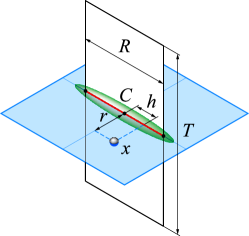
Figure 1: (Color online) The geometry of our simulations. The topological/action densities are calculated at the point $(r,h)$, where $r$ and $h$ are, respectively, the transverse and longitudinal coordinates with respect to the geometrical center $C$ of the rectangular $T\times R$ Wilson loop.

The geometry relevant to the correlation functions (6), (7) is shown in Figure 1. For the rectangular $T\times R$ Wilson loop the chromoelectric string appears between the static quark-antiquark pair at the moment $t=0$. Once created, the string develops in full at the time $t=T/2$ when the numerical evaluation of the string profile is performed. Finally, the string disappears at the time $t=T$ when the quark and the antiquark are annihilated. For large enough $T$ the problem evidently possesses spacial cylindrical symmetry, which suggests to use coordinates $x=(r,h)$, where $r$ and $h$ are, respectively, the transverse and longitudinal distances to the geometrical string center $C$.

As is well known, at the quantum-mechanical level the string must fluctuate around classical (minimum action) configuration. Lüscher Luscher:1980iy has obtained long ago a quantitative estimation of the quantum fluctuations of a bosonic string. According to Ref. Luscher:1980iy one generally expects that the deviation of the string position with respect to its classical limit should follow a Gaussian distribution with a calculable width. The quantum fluctuations of the string should also affect distributions of all other quantities associated with the string. In particular, the profiles of the action and topological densities should become noticeably wider due to the string fluctuations compared to the that for the classical (non-fluctuating) string. Therefore, one expects generically that the transverse slices of the correlation functions (6), (7) at the geometrical center $h=0$ of the string should follow the Lüscher scaling law:

$$X_{\cal C}(r,R)=-C_{X}(R)\,\exp\Bigl{\{}-\frac{r^{2}}{\delta^{2}_{X}(R)}\Bigr{\}}\,,$$ (10)

where $X$ stands for either the topological charge or the action, $X=Q,S$. This distribution is characterized by two quantities which are the amplitude $C_{X}$ and the width $\delta_{X}$ of the transverse string fluctuations. Note that both these quantities depend in general on the length of the string $R$. In particular, the squared width of the bosonic string is known Luscher:1980iy to increase logarithmically for sufficiently long strings:

$$\delta^{2}_{X}(R)=\frac{\zeta_{X}}{\pi\sigma}\ln\frac{R}{R^{\mathrm{core}}_{X}}\,.$$ (11)

Here $\sigma$ is the tension of the string and $\zeta_{X}$ is a coefficient of proportionality which is expected to be unity in $(3+1)$ dimensions

$$\zeta_{X}=1\,.$$ (12)

Note that the range of qualitative applicability of the result (10) is dictated by purely geometrical reasons: the length $R$ of the string should be larger than some critical value $R^{\mathrm{core}}_{X}$ of order of the string width. In the case of unprojected action density, which is related to the heavy quark potential via the action sum rules ref:sum-rules , one assumes that the coefficient $\sigma$ in Eq. (11) equals to the physical string tension. For the ${\mathrm{HP}^{1}}$-projected action density we also expect the same: although the sum rules are not applicable any longer, physics-wise it seems natural that $\sigma$ must be equal to the ${\mathrm{HP}^{1}}$-projected string tension. However, for the topological density the arguments break down and the scale of the width of the topological fluctuations in the vicinity of the string should be examined in the numerical simulations.

IV Details of Numerical Simulations

$\beta$ $a\sqrt{\sigma_{\mathrm{full}}}$ $a\sqrt{\sigma_{\mathrm{HP}}}$ $N^{\mathrm{conf}}$ $V^{\mathrm{lat}}$ $V^{\mathrm{phys}}\cdot\sigma^{2}_{\mathrm{HP}}$ 2.510 0.176(2) 0.119(3) 60 $32^{4}$ $[3.8(1)]^{4}$ 2.600 0.131(2) 0.105(2) 70 $28^{4}$ $[2.9(1)]^{4}$

Table 1: The parameters of our simulations.

Our measurements were performed on two sets (Table 1) of statistically independent $SU(2)$ gauge configurations generated with standard Wilson action. These thermalized gauge ensembles were used only to produce the embedded ${\mathrm{HP}^{1}}$ $\sigma$-model configurations, the procedure being exactly the same as in the second paper of Ref. Gubarev:2005rs . The physical scale for the obtained $\sigma$-model data sets could be fixed by the requirement that either the full string tension $\sigma_{\mathrm{full}}$ or its ${\mathrm{HP}^{1}}$-projected counterpart $\sigma_{\mathrm{HP}}$ equals to the conventional value $(440~{}\mathrm{MeV})^{2}$. Physically these two prescriptions are equivalent since it is known that the ${\mathrm{HP}^{1}}$-projected string tension coincides with the full one in the continuum limit. However, at necessarily finite $\beta$ values a particular choice might be preferable for scaling checks. For us the prescription $\sqrt{\sigma_{\mathrm{full}}}=440~{}\mathrm{MeV}$ seems to be unnatural since after all the original gauge configurations were not used in the measurements. What is physically relevant in the present context is the ${\mathrm{HP}^{1}}$-projected string tension and we set the scale by fixing $\sigma_{\mathrm{HP}}$ to the above value. Note that since this prescription differs from the conventional one we use the dimensionless combinations like $R\sqrt{\sigma_{\mathrm{HP}}}$ instead of the usual fermi units.

The string profiles may obviously be affected by the finiteness of the temporal extension $T$. To reduce these finite-time effects we used the conventional APE-smearing procedure ref:smearing for spatial pieces of the trajectory ${\cal C}$ and checked independence of our results against variation of $T$. The geometrical setup described above makes it convenient to consider Wilson loops of only even temporal and spacial extents in lattice units. Furthermore, the non-locality issue, Eq. (5), forces us to disregard the smallest loops. Thus we confined ourselves to planar $T\times R$ Wilson contours with $T,R=4,...,14$ with understanding that $T,R=4,6$ data points must be used with care.

V Topological Density in the String

The qualitative topological portrait of the confining string is revealed by the correlation function (6), shown in Figure 2 for our $\beta=2.60$ data set. As is apparent from this Figure the quantity $Q_{\cal C}$ is always negative in the vicinity of the string while approaching zero far away from quark-antiquark pair. Thus the confining flux tube suppresses the topological fluctuations. Note also that the suppression is maximal at the positions of quarks, which are sitting at the absolute minima of the topological density profile (this observation is in agreement with Ref. string:topcharge:first ; string:topcharge ). Moreover, the quarks look like the sources of Coulomb potential in the topological density, which by itself a rather striking result especially in view of the corresponding action density profile to be discussed below.

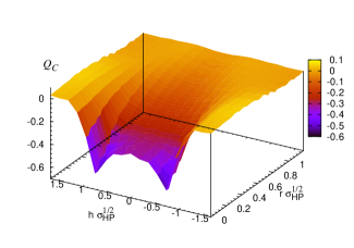
Figure 2: (Color online) Correlation function (6) at quark-antiquark separation $R\sqrt{\sigma_{\mathrm{HP}}}=1.47(3)$ measured on $\beta=2.60$ data set. Temporal extent of the Wilson loop is $T\sqrt{\sigma_{\mathrm{HP}}}=1.05(2)$.

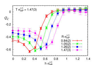
Figure 3: (Color online) The longitudinal slices ($r=0$) of the topological density correlation function (6) at various quark-antiquark separations $R$ at $\beta=2.60$. Only the positive half ($h\geqslant 0$) of the axis is shown, lines are plotted to guide the eye.

The typical longitudinal ($r=0$) slices of the topological density correlation function (6) are plotted in Figure 3 for various lengths $R$ of the confining string. The minima of the topological density are reached in the vicinities of the quark and anti-quark, $h_{\min}\approx R/2$. As one goes outward the string, $h>h_{\min}$, the quantity $Q_{\cal C}$ rapidly approaches zero indicating that topological charge density quickly comes to its vacuum expectation value outside the string. To the contrary, if one moves toward the string center, $h\to 0$, the magnitude of $Q_{\cal C}$ remains negative slowly approaching its limiting value at $h=0$.

The degree of the suppression of the topological density at the geometrical center of the string $r=h=0$ varies with the string length. This property is visualized for both our data sets and for various temporal extensions $T$ of the Wilson loops on Figure 4. One can see that the topological density at the string center tend to its vacuum value as the string gets longer. This feature is in agreement with the picture of the fluctuating string: as the string gets longer its transverse fluctuations increase in amplitude and the string gets more dispersed in the space. As the consequence, the correlation of all quantities (including the topological charge density) with the string gets weaker at the geometrical center with increasing string length.

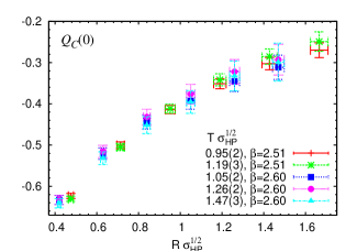
Figure 4: (Color online) The topological density correlation function (6) at the geometrical center of the string ($h=r=0$) versus the quark separation $R$ for the Wilson loops of various temporal extension.

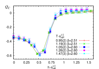
Figure 5: (Color online) Example of the longitudinal profiles at $r=0$ of the correlator (6) at string lengths $R\sqrt{\sigma_{\mathrm{HP}}}=1.19(3)$ for $\beta=2.51$ and $R\sqrt{\sigma_{\mathrm{HP}}}=1.26(2)$ for $\beta=2.60$ and various time extensions of the Wilson loop.

Another information imprinted in Figure 4 is small sensitivity of the central value of the topological density correlator (6) against the variation of the temporal extent of the Wilson loop $T$. The typical dependence of the string profile for $h>0$ on the time extension of the Wilson loop is presented on Figure 5 for the quark-antiquark separations $R\sqrt{\sigma_{\mathrm{HP}}}=1.19(3)$ (data set $\beta=2.51$) and $R\sqrt{\sigma_{\mathrm{HP}}}=1.26(2)$ ($\beta=2.60$). It is seen that the string profile is indeed robust against the time passed between creation and annihilation of the quark pair. Therefore we conclude that within our accuracy the dependence of the results on the time extension $T$ is negligible.

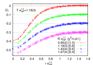
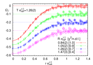
Figure 6: (Color online) The distributions of the topological charge fluctuations (6) in the transverse direction $r$ around the geometrical string center $h=0$. For the sake of clarity the data points were $y$-shifted, and the corresponding $Q_{\cal C}=0$ levels are shown by thin horizontal lines. Upper and lower panels refer, respectively, to the $\beta=2.51$ and $\beta=2.60$ data sets. Best fits by the Gaussian function (10) are shown by thick lines. The string lengths $R$, the temporal extensions $T$ and the reduced $\chi^{2}$ values are indicated as well.

In order to check the validity of the Lüscher formula (10) for the width of the topological charge fluctuations around the string we fitted the transverse slice of the correlation function (6) at the string center $h=0$ by the Gaussian ansatz (10). We find that the scaling law (10) well describes both our data sets as one can see from various examples of the fits shown in Figure 6. The only notable deviations from (10) was observed for small string lengths, $R\sqrt{\sigma_{\mathrm{HP}}}\lesssim 0.7$, which, however, is to be expected since Eq. (10) is valid only for large $R$. Therefore in terms of the topological density the string formation length, at which the asymptotic behavior (10) settles in, could be estimated as $R\sqrt{\sigma_{\mathrm{HP}}}\approx 0.7$ and is in agreement both with the literature Bali:1994de and with the corresponding result coming from the action density profiles (see below). In turn, the Gaussian fits allow to obtain the corresponding parameters. On the bottom panel of Figure 7 we plot the squared string width $\delta^{2}_{Q}(R)$ obtained for $\beta=2.60$ data set as a function of the string length $R$ for various temporal extensions $T$ of the Wilson contour.

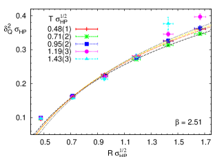
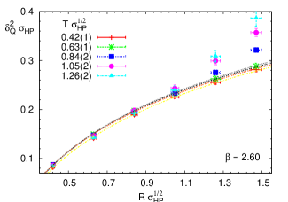
Figure 7: (Color online) The squared string width $\delta^{2}_{Q}$ vs. the string length $R$ for various time extensions of the Wilson contour. Data points had been obtained with $\beta=2.51$ (top) and $\beta=2.60$ (bottom) sets. The lines represent the best fits by the function (11) (the details are given in the text).

One obvious thing to note here is that $\delta^{2}_{Q}(R)$ data points are indeed compatible with logarithmic dependence (11) in the whole $R$ interval for small $T\sqrt{\sigma_{\mathrm{HP}}}=0.42(1),0.63(1)$, while for $T\sqrt{\sigma_{\mathrm{HP}}}\gtrsim 0.84(2)$ they start to deviate from (11) for large string lengths. In fact, for $T\sqrt{\sigma_{\mathrm{HP}}}=0.84(2),1.05(2)$ the total set of $R$ data points corresponds rather to the linear dependence of $\delta^{2}_{Q}$ on $R$, which is presumably a manifestation of finite size effects. Indeed, the considerations Bali:1994de showing that finite size corrections are negligible even for largest loops are not applicable in our case: for ${\mathrm{HP}^{1}}$ $\sigma$-model induced gauge fields the relevant center symmetry transformations do not exist. Therefore the finite volume effects are expected to be much more severe than they are in usual approaches and indeed at largest available $T\sqrt{\sigma_{\mathrm{HP}}}=1.26(2)$ the squared string width increases with $R$ even more rapidly showing somewhat irregular behavior for large quark-antiquark separations. We attribute the deviation of the string width from logarithmic law to the boundary conditions in the temporal and spatial directions: the long enough string interacts with its temporal and spatial replicas. The strength of this artificial interaction is rising with increase of the area of the string worldsheet achieved at large $R$ and $T$. The assumption of strong finite volume effects present for $\beta=2.60$ configurations is justified below (see also Section VI). However, for small $T$ the finite volume corrections are surely negligible, which permits us to fit $\delta^{2}_{Q}(R)$ to Eq. (11) in the range $R\sqrt{\sigma_{\mathrm{HP}}}\gtrsim 0.7$ for $T\sqrt{\sigma_{\mathrm{HP}}}=0.42(1),0.63(1)$ and in the interval $0.7\lesssim R\sqrt{\sigma_{\mathrm{HP}}}<1.2$ at $T\sqrt{\sigma_{\mathrm{HP}}}=0.84(2),1.05(2)$. The lower bound on $R$ is due to Eq. (5) and because the Gaussian fit (10) is not adequate at small distances resulting in rather large $\chi^{2}$ values. The outcome of these fits is used below.

In order to check finite volume effects we performed the same calculations on our $\beta=2.51$ configurations, for which the physical volume is much larger. The results are presented on the top panel of Figure 7, from which it is apparent that the data points are much more stable in this case. Namely, the dependence $\delta^{2}_{Q}(R)$ follows the logarithmic law (11) up to the time scale of order $T\sqrt{\sigma_{\mathrm{HP}}}\lesssim 1.2$. However, at even larger $T$ we again see notable deviations from Eq. (11) the source of which is not so evident for us at present. Most probably, the errors bars are underestimated for the corresponding largest Wilson loops and much more statistics in needed to confirm (11) at $T\sqrt{\sigma_{\mathrm{HP}}}\gtrsim 1.2$, $R\sqrt{\sigma_{\mathrm{HP}}}\gtrsim 1.4$.

To summarize, our numerical data on the string width obtained from the topological density correlation function (6) indeed favors the logarithmic widening (11) of the confining string. Unfortunately, $\beta=2.60$ data set has relatively small physical volume which disturbs the expected dependence $\delta^{2}_{Q}(R)$. Anyway, for not so large time extent of the Wilson loops logarithmic string broadening is clearly seen. As far as the measurements at $\beta=2.51$ are concerned, the corresponding physical volume is much larger and the logarithmic widening is confirmed for much larger Wilson loops.

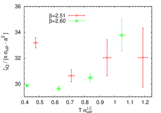
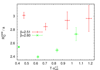
Figure 8: (Color online) The coefficients $\zeta_{Q}/[\pi\sigma_{\mathrm{HP}}\cdot a^{2}]$ (top) and $R^{\mathrm{core}}_{Q}/a$ (bottom) of the Lüscher scaling law (11) as determined from Wilson loops of various time extension $T$ for both our data sets. Note that all quantities are given in the lattice units.

The fits of the Gaussian string profiles (10) allow us to estimate the dimensionless parameters $\zeta_{Q}$ and $R^{\mathrm{core}}_{Q}$ of the Lüscher scaling law (11). According to the theoretical expectation the parameter $\zeta_{Q}$ must of order one provided that the width $\delta_{Q}$ is given in terms of the physical string tension, while there are essentially no theoretical predictions for the string core width $R^{\mathrm{core}}_{Q}$. However, the relevant question for both quantities is whether they are given in physical units or are of order lattice spacing. In the upper and lower panels of Figure 8 we plot the parameters $\zeta_{Q}/[\pi\sigma_{\mathrm{HP}}\cdot a^{2}]$ and $R^{\mathrm{core}}_{Q}/a$, respectively, obtained by the logarithmic fits (11) as a functions of the temporal string extension $T$. It is apparent that $T$-dependence is indeed mild in both cases. At the same time, it is essential that the parameters are expressed in the units of UV cutoff, which we found the only possibility to make $\beta=2.51$ and $\beta=2.60$ data points qualitatively consistent. Hence the string width and the size of the string core, as they are seen by the topological fluctuations, are likely to be at the scale of the lattice spacing. Unfortunately, this result is mainly qualitative and is not fairly convincing because we consider only two lattice spacings while the logarithmic fits are weakly sensitive to variations of $R^{\mathrm{core}}_{Q}$. For these reasons we refrain from definite conclusions since more data is needed to clarify the issue.

VI Action Density in the String

In this Section we repeat the above investigations of the string profiles using the ${\mathrm{HP}^{1}}$-projected action density

$$s=\mathop{\rm Tr}F^{\mathrm{HP}}_{\mu\nu}F^{\mathrm{HP}}_{\mu\nu}\,,$$ (13)

where the inessential normalization factor was omitted. Note that in this case the obtained statistics is much better allowing more precise analysis. The typical distribution of the action density around the string is presented on Figure 9.

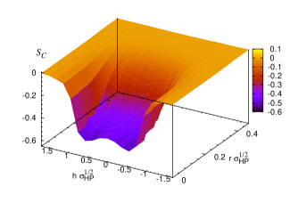
Figure 9: (Color online) The action density correlation function (7) measured on $\beta=2.51$ configurations for the string length $R\sqrt{\sigma_{\mathrm{HP}}}=1.67(4)$ and for the temporal extension of the Wilson loop $T\sqrt{\sigma_{\mathrm{HP}}}=1.19(3)$.

It is clear from the figure that the action density is indeed suppressed in the vicinity of the string in agreement with the analogous result for unprojected fields ref:sum-rules . At the same time, there are a few noticeable differences between the action density profile of the string and the corresponding topological charge correlation function, Figure 2. First, the positions of the test quark and the anti-quark are explicitly noticeable in the string topological profile as these positions correspond to the two global minima of $Q_{\cal C}$. However, the location the test charges in the action density correlator is not seen clearly. Second, the transverse distribution of the action is seemingly wider compared to the one of the topological charge. Finally, the data for the action comes with much less noise compared to one of the topological distribution at the same numerical statistics.

In order to illustrate the above observations we plot in Figure 10 the longitudinal profiles of the action density and compare them with the same quantity for the topological charge plotted in Figure 3.

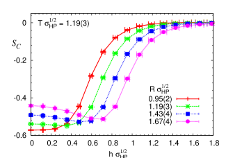
Figure 10: (Color online) The longitudinal profile ($r=0$) of the action density correlator $S_{\cal C}$ obtained with $\beta=2.51$ data set. The positive half ($h\geqslant 0$) of the axis is shown for various indicated string lengths $R$. The lines are plotted to guide eye.

One notices that the global minimum of the quantity $S_{\cal C}$ shifts with increasing distance between test color charges, being located at the string center point for relatively small $R$. As $R$ enlarges the minimum shifts roughly to the string end-point, however, it remains much wider compared to that of the topological density. This property is also illustrated in Figure 11 in which the correlation function (6) at the geometrical center $r=h=0$ of the string is plotted as a function of the string length $R$.

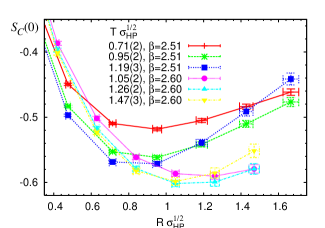
Figure 11: (Color online) The action density (6) at the center of the string ($h{=}r{=}0$) vs. the string length $R$ at various time extensions $T$.

We conclude qualitatively that the location of the quarks becomes visible in the longitudinal action density profile at string length about $R\sqrt{\sigma_{\mathrm{HP}}}\approx 1.0$. Note that the apparent discrepancy in this number between $\beta=2.51$ and $\beta=2.60$ data points is presumably due to the finite volume effects discussed in previous section.

As it was done in the case of the topological charge, we study the transverse slices of the action density correlation function (7) at the geometrical center $h=0$ of the string. Generically, one expects that the Gaussian distribution (10) should adequately describe the data provided that the string length is large enough. It turns out that indeed the transverse action density distribution around the string obeys (10) for $R\sqrt{\sigma_{\mathrm{HP}}}\gtrsim 0.7$ as is illustrated on Figure 12.

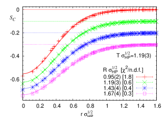
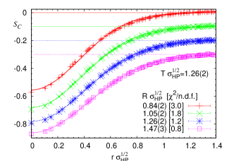
Figure 12: (Color online) Transverse slices of the action density correlation function (7) at the geometrical center of the string $h=0$ for various temporal $T$ and spacial $R$ extensions of the Wilson contour. Upper (lower) panel refers to $\beta=2.51$ ($\beta=2.60$) data set. For clarity reasons data points were $y$-shifted by $-0.1$, $-0.2$ and $-0.3$ (the corresponding $S_{\cal C}=0$ levels are shown by thin horizontal lines). The fits of the distributions by the Gaussian function (10) are shown by thick lines.

For smaller string lengths the data shows significant deviations from the Gaussian ansatz indicating that the string formation length is not reached yet. Therefore, the string width could be extracted reliably from fits only for $R\sqrt{\sigma_{\mathrm{HP}}}>0.7$ and in the considerations below we restrict ourselves to these distances.

As far as the parameters of the Gaussian distribution are concerned, we plot the corresponding squared width of the action density profile obtained at various $R$ and $T$ on Figure 13.

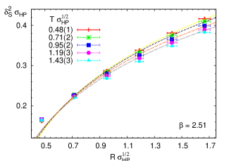
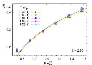
Figure 13: (Color online) The squared string width $\delta^{2}_{S}$ vs. the string length $R$ for various time extensions $T$ of the Wilson contour. Data points corresponds to $\beta=2.51$ (top) and $\beta=2.60$ (bottom) sets. The lines represent the best fits to (11).

As is apparent from that Figure, the data points for $\delta^{2}_{S}(R)$ at each $\beta$-value confirm the logarithmic string widening for all available $T$ in the entire range of quark-antiquark separations beyond the string formation length. Moreover, the function $\delta^{2}_{S}(R)$ appears to depend very mildly on $T$. However, basing on our experience with the topological density distribution we excluded from our analysis the largest $T$ data points, which presumably suffer from finite volume corrections.

Next we estimate the parameters $\zeta_{S}$ and $R^{\mathrm{core}}_{S}$ entering the logarithmic scaling law (11). To this end, we fitted the $\delta^{2}_{S}(R)$ dependence to Eq. (11) in the range $R\sqrt{\sigma_{\mathrm{HP}}}\geq 0.7$ for $T$ values, for which the finite volume corrections are expected to be small, namely, for $T\sqrt{\sigma_{\mathrm{HP}}}<1.0$ on $\beta=2.51$ configurations and for $T\sqrt{\sigma_{\mathrm{HP}}}=0.42(1),0.63(1)$ with $\beta=2.60$ data set. For larger temporal extensions of the Wilson loops we restricted the fitting range from above, $R\sqrt{\sigma_{\mathrm{HP}}}\lesssim 1.3$, although we checked that inclusion of largest $R$ points changes the results at most by $\sim 10\%$. The outcome of the fits is presented on Figure 14. As might be expected, the amplitude of the logarithmic widening seems to be given indeed in physical units, as is illustrated on the top panel of Figure 14.

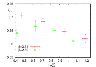
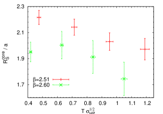
Figure 14: (Color online) The coefficients $\zeta_{S}$ (top) and $R^{\mathrm{core}}_{S}/a$ (bottom) of the Lüscher scaling law (11) as determined from Wilson loops of various time extensions $T$ calculated at both available data sets. Note that $\zeta_{S}$ is shown in physical units with the normalization $\sigma=\sigma_{\mathrm{HP}}$, while $R^{\mathrm{core}}_{S}$ is plotted in the lattice units.

Namely, if we assume that the string width scale $\sigma$, Eq. (11), equals to the projected string tension $\sigma_{\mathrm{HP}}$ then the corresponding dimensionless coefficient $\zeta_{S}$ appears to be spacing independent and is about unity. However, the data for string core width favors again the constancy of $R^{core}_{S}$ in lattice units, the value of which is close to one obtained from the topological density profiles (see the bottom panel of Figure 14). Note that due to the generically expected small sensitivity of logarithmic fits to $R^{core}_{S}$, our statistics and the spacing variations considered might be insufficient to determine accurately the width of the string core. Hence at present we cannot fairly insist on the relation $R^{core}_{S}\sim a$, new measurements are needed to confirm it.

To summarize, the measurements of the action density correlation function (7) confirm the logarithmic widening of the confining string. Moreover, we were able to demonstrate that the string broadening is in agreement with general theoretical expectations and is qualitatively compatible with the bosonic string picture of the confining flux tube. However, the data for the string core width, where the string widening settles in, is less conclusive and favors rather small value of $R^{core}_{S}$ of order lattice spacing. In particular, even if one would insist that $R^{core}_{S}$ is given in physical units, then its numerical value is about

$$R^{\mathrm{core}}_{S}\approx 0.1~{}\mathrm{fm}\,.$$ (14)

Note that Eq. (14) is in qualitative agreement with the literature. Indeed, it had been shown in Refs. Luscher:2002qv ; Juge:2002br that the transition from perturbative to stringy description of quark-antiquark pair happens at rather small distances of order $0.2\div 0.3~{}\mathrm{fm}$ Luscher:2002qv . The early start of the string regime was also found in Ref. Panero:2005iu in compact $U(1)$ gauge theory in four space-time dimensions. It could well be that the early onset of the string fluctuations is a universal feature of the theories possessing string excitations.

VII Discussion and Conclusion

In this paper we investigated the topological and the action density profiles of the confining string in pure $SU(2)$ Yang-Mills theory on the lattice using the method of the quaternionic projective $\sigma$-model embedding. Indeed, the main difficulty in the conventional considerations is caused by UV dominated zero-point fluctuations, which give identically vanishing but numerically destructive contribution to the correlation functions of the topological/action density and the confining flux tube. On the other hand, the ${\mathrm{HP}^{1}}$ $\sigma$-model embedding and corresponding gauge covariant ${\mathrm{HP}^{1}}$-projection procedure allows to filter out essentially the only leading power divergences from local observables in question, leaving intact the subleading and the IR dominated contributions. At very least this property ${\mathrm{HP}^{1}}$ embedding is known to hold in numerical simulations and hence allows to obtain rather accurate results for the topological and action density profiles of the confining string. It is worth mentioning that the known disadvantages of ${\mathrm{HP}^{1}}$ embedding are expected to play no role in the problem considered. Indeed, the finite non-locality range of the approach should be inessential for large enough Wilson loop, which are relevant for the present investigation. Moreover, our results are in agreement with the existing literature, when the comparison is possible.

Our paper presents the first quantitative investigation of the topological density distribution in the vicinity of the chromoelectric string. Although it had been known for some time string:topcharge:first ; string:topcharge that confining string suppresses the topological fluctuations, we were able to investigate the problem in details and to show, in particular, that the confining flux tube in terms of the topological density corresponds likely to the fluctuating string. Moreover, we confirmed the generically expected logarithmic string widening and we attempted also to estimate the characteristic string scales. Our data seems to indicate that in terms of the topological density the confining flux tube is rather thin object stretched in between quark-antiquark pair. Although at present we cannot fairly insist on this picture and more data is obviously needed to confirm the result, nevertheless, it is rather striking and theoretically challenging by itself. We hope to shed more light on the issue in forthcoming publications.

As far as the action density profiles are concerned, the use of the projected action density allowed us to obtain rather accurate results confirming the string picture. In this case, the string formation and its logarithmic widening is also established. Moreover, the characteristic width of the flux tube is shown to be given in physical units and the features of its broadening seem to be compatible with the effective bosonic string description.

- (1) G. S. Bali, C. Schlichter and K. Schilling, Phys. Rev. D 51, 5165 (1995).
- (2) G. S. Bali, Phys. Rept. 343, 1 (2001); G. S. Bali, “The mechanism of quark confinement”, in “Newport News 1998, Quark confinement and the hadron spectrum III” p. 17, Ed. by Nathan Isgur (Singapore, World Scientific, 2000), arXiv:hep-ph/9809351.
- (3) R. W. Haymaker, V. Singh, Y. C. Peng and J. Wosiek, Phys. Rev. D 53, 389 (1996); T. T. Takahashi, H. Suganuma, Y. Nemoto and H. Matsufuru, Phys. Rev. D 65, 114509 (2002); F. Okiharu and R. M. Woloshyn, Nucl. Phys. Proc. Suppl. 129, 745 (2004); A. M. Green, C. Michael and P. S. Spencer, Phys. Rev. D 55, 1216 (1997); A. M. Green, P. S. Spencer and C. Michael, in “Como 1996, Quark confinement and the hadron spectrum II”, p.289, Ed. by N. Brambilla and G.M. Prosperi (River Edge, NJ, World Scientific, 1997), arXiv:hep-lat/9609019.
- (4) F. Bissey et al., Nucl. Phys. Proc. Suppl. 141, 22 (2005); F. Bissey, F. G. Cao, A. R. Kitson, A. I. Signal, D. B. Leinweber, B. G. Lasscock and A. G. Williams, arXiv:hep-lat/0606016.
- (5) V.G. Bornyakov et al. Phys. Rev. D 70, 054506 (2004); V.G. Bornyakov et al., Prog. Theor. Phys. 112, 307 (2004).
- (6) F. Karsch, Nucl. Phys. B 205, 285 (1982); C. Michael, Nucl. Phys. B 280, 13 (1987); H. G. Dosch, O. Nachtmann and M. Rueter, arXiv:hep-ph/9503386; H. J. Rothe, Phys. Lett. B 355, 260 (1995); H. J. Rothe, Phys. Lett. B 364, 227 (1995).
- (7) M. N. Chernodub et al., Phys. Rev. D 72, 074505 (2005).
- (8) M. J. Lavelle, M. Schaden, Phys. Lett. B 208, 297 (1988); P. Boucaud, A. Le Yaouanc, J. P. Leroy, J. Micheli, O. Pene, J. Rodriguez-Quintero, Phys. Lett. B 493, 315 (2000); F. V. Gubarev, L. Stodolsky, V. I. Zakharov, Phys. Rev. Lett. 86, 2220 (2001); F. V. Gubarev, V. I. Zakharov, Phys. Lett. B 501, 28 (2001).
- (9) Y. Nambu, Phys. Rev. D 10, 4262 (1974); G. ’t Hooft, in Proceedings of the EPS International Conference, edited by A. Zichichi, p. 1225 (1976); S. Mandelstam, Phys. Rept. 23, 245 (1976).
- (10) T. Suzuki, Nucl. Phys. Proc. Suppl. 30, 176 (1993); M. N. Chernodub, M. I. Polikarpov, “Abelian projections and monopoles”, in ”Confinement, duality, and nonperturbative aspects of QCD”, Ed. by P. van Baal, Plenum Press, p. 387, hep-th/9710205; R.W. Haymaker, Phys. Rept. 315, 153 (1999).
- (11) E. Laermann and P. Schildberg, Nucl. Phys. Proc. Suppl. 30, 503 (1993).
- (12) W. Sakuler, W. Burger, M. Faber, H. Markum, M. Muller, P. De Forcrand, A. Nakamura, I.O. Stamatescu, Phys. Lett. B 276, 155 (1992).
- (13) M. Faber, H. Markum, S. Olejnik and W. Sakuler, Phys. Lett. B 334, 145 (1994).
- (14) S. Thurner, M. Feurstein, H. Markum, W. Sakuler, Phys. Rev. D 54, 3457 (1996).
- (15) H. Neuberger, Phys. Lett. B 417, 141 (1998); H. Neuberger, Phys. Lett. B 427, 353 (1998); R. Narayanan and H. Neuberger, Nucl. Phys. B 443, 305 (1995); P. Hasenfratz, V. Laliena and F. Niedermayer, Phys. Lett. B 427, 125 (1998); D. H. Adams, Annals Phys. 296, 131 (2002); R. Narayanan and P. M. Vranas, Nucl. Phys. B 506, 373 (1997).
- (16) I. Horvath et al., Phys. Lett. B 617, 49 (2005).
- (17) I. Horvath et al., Phys. Rev. D 66, 034501 (2002); Phys. Rev. D 67, 011501 (2003); Phys. Rev. D 68, 114505 (2003).
- (18) F. V. Gubarev and S. M. Morozov, Phys. Rev. D 72, 076008 (2005); P. Y. Boyko, F. V. Gubarev and S. M. Morozov, Phys. Rev. D 73, 014512 (2006).
- (19) P. Y. Boyko and F. V. Gubarev, Phys. Rev. D 73, 114506 (2006).
- (20) F. Bruckmann, C. Gattringer, E. M. Ilgenfritz, M. Muller-Preussker, A. Schafer and S. Solbrig, arXiv:hep-lat/0612024; C. Gattringer, E. M. Ilgenfritz and S. Solbrig, arXiv:hep-lat/0601015.
- (21) M. Luscher, G. Munster and P. Weisz, Nucl. Phys. B 180, 1 (1981).
- (22) M. Caselle, F. Gliozzi, U. Magnea and S. Vinti, Nucl. Phys. B 460, 397 (1996);
- (23) M. Caselle, M. Hasenbusch and M. Panero, JHEP 0301, 057 (2003); M. Caselle, M. Panero and P. Provero, ibid. 0206, 061 (2002).
- (24) V. G. Bornyakov et al. [DIK Collaboration], Phys. Rev. D 70, 074511 (2004).
- (25) L. Del Debbio, M. Faber, J. Greensite and S. Olejnik, Phys. Rev. D 55, 2298 (1997); J. Greensite, Prog. Part. Nucl. Phys. 51, 1 (2003).
- (26) V. G. Bornyakov, A. V. Kovalenko, M. I. Polikarpov and D. A. Sigaev, Nucl. Phys. Proc. Suppl. 129, 757 (2004).
- (27) M. S. Narasimhan, S. Ramanan, Amer. Journ. of Math. 85, 223 (1963).
- (28) F. Gursey and C. H. Tze, Annals Phys. 128, 29 (1980); J. Lukierski, CERN-TH-2678; Y. N. Kafiev, Phys. Lett. B 87 (1979) 219; Nucl. Phys. B 178, 177 (1981); M. A. Jafarizadeh, M. Snyder and C. H. Tze, Nucl. Phys. B 176, 221 (1980); D. Maison, MPI-PAE/PTh 52/79; J. E. Avron, L. Sadun, J. Segert and B. Simon, Comm. Math. Phys. 124, 595 (1989); M. T. Johnsson and I. J. R. Aitchison, J. Phys. A 30, 2085 (1997); E. Demler and S. C. Zhang, Annals Phys. 271, 83 (1999); M. F. Atiyah, N. J. Hitchin, V. G. Drinfeld and Y. I. Manin, Phys. Lett. A 65, 185 (1978); V. G. Drinfeld and Y. I. Manin, Commun. Math. Phys. 63, 177 (1978); M. Dubois-Violette, Y. Georgelin, Phys. Lett. B 82, 251 (1979).
- (29) I. Horvath et al., Nucl. Phys. Proc. Suppl. 129, 677 (2004); Phys. Lett. B 612, 21 (2005); A. Alexandru, I. Horvath, J. Zhang, Phys. Rev. D 72, 034506 (2005); I. Horvath, Nucl. Phys. B 710, 464 (2005) [Erratum-ibid. B 714, 175 (2005)]; C. Gattringer, M. Gockeler, P. E. L. Rakow, S. Schaefer and A. Schafer,Nucl. Phys. B 617, 101 (2001); C. Aubin et al., Nucl. Phys. Proc. Suppl. 140, 626 (2005); C. Bernard et al., PoS LAT2005, 299 (2005).
- (30) Y. Koma, E. M. Ilgenfritz, K. Koller, G. Schierholz, T. Streuer and V. Weinberg, PoS LAT2005, 300 (2005); arXiv:hep-lat/0611007; arXiv:hep-lat/0610087; F. V. Gubarev, S. M. Morozov, M. I. Polikarpov and V. I. Zakharov, JETP Letters 82, 381 (2005); PoS LAT2005, 143 (2005).
- (31) A. M. Polyakov, Mod. Phys. Lett. A 3, 325 (1988); P. B. Wiegmann, Phys. Rev. Lett. 60, 821 (1988); H. B. Nielsen and D. Rohrlich, Nucl. Phys. B 299, 471 (1988); L. Schulman, Phys. Rev. 176, 1558 (1968); G. P. Korchemsky, Int. J. Mod. Phys. A 7, 339 (1992); Phys. Lett. B 232, 334 (1989); T. Jaroszewicz and P. S. Kurzepa, Annals Phys. 210, 255 (1991); J. Ambjorn, B. Durhuus and T. Jonsson, Nucl. Phys. B 330, 509 (1990); J. Grundberg, T. H. Hansson and A. Karlhede, Phys. Rev. D 41, 2642 (1990).
- (32) C. Csaki, H. Ooguri, Y. Oz and J. Terning, JHEP 9901, 017 (1999); J. Erlich, E. Katz, D. T. Son and M. A. Stephanov, Phys. Rev. Lett. 95, 261602 (2005); L. Da Rold and A. Pomarol, Nucl. Phys. B 721, 79 (2005); N. Evans, J. P. Shock and T. Waterson, Phys. Lett. B 622, 165 (2005); E. Katz, A. Lewandowski and M. D. Schwartz, Phys. Rev. D 74, 086004 (2006); A. Karch, E. Katz, D. T. Son and M. A. Stephanov, Phys. Rev. D 74, 015005 (2006); C. Csaki and M. Reece, arXiv:hep-ph/0608266; O. Andreev and V. I. Zakharov, Phys. Rev. D 74, 025023 (2006); JHEP 0704, 100 (2007); Phys. Lett. B 645, 437 (2007).
- (33) M. Albanese et al. [APE Collaboration], Phys. Lett. B 192, 163 (1987).
- (34) M. Luscher and P. Weisz, JHEP 0207, 049 (2002).
- (35) K. J. Juge, J. Kuti and C. Morningstar, Phys. Rev. Lett. 90, 161601 (2003).
- (36) M. Panero, JHEP 0505, 066 (2005).