CERN-PH-TH/2007-030
DESY 07-005
KEK-CP-192
UTHEP-539
COLO-HEP-522
Non-perturbative improvement of the axial current with three dynamical flavors and the Iwasaki gauge action

Abstract

We perform a non-perturbative determination of the improvement coefficient $c_{\rm A}$ to remove $O(a)$ discretization errors in the axial vector current in three-flavor lattice QCD with the Iwasaki gauge action and the standard O$(a)$-improved Wilson quark action. An improvement condition with a good sensitivity to $c_{\rm A}$ is imposed at constant physics. Combining our results with the perturbative expansion, $c_{\rm A}$ is now known rather precisely for $a^{-1}\!\gtrsim\!1.6$ GeV.

1 Introduction

Various discretizations of QCD on a lattice are presently used in the large scale efforts aiming at non-perturbative results in the theory of strong interactions (see [1, 2, 3, 4, 5, 6, 7, 8, 9, 10] and references therein). Wilson’s original formulation [11] is theoretically very well founded [12, 13] and rather simple to implement in numerical simulations. The flavor symmetries are exact and with modern algorithms [14, 15, 16, 17, 18] the regime of small quark masses and small lattice spacings can be reached [1, 19]. On the other hand it is well known that since the chiral symmetries are broken by the Wilson term, lattice artifacts linear in the lattice spacing are present. It has long been understood how these can be removed by applying Symanzik’s improvement programme [20, 21, 22, 23, 24]. One has to add dimension five fields to the lattice Lagrangian and (for example) dimension four fields to the quark bilinears. In particular the bare flavor axial current

$$A_{\mu}^{a}(x)=\overline{\psi}(x)\,T^{a}\,\gamma_{\mu}\gamma_{5}\,\psi(x)$$ (1)

(the SU($N_{\rm f}$) generator $T^{a}$ acts in flavor space) is improved by

$$(A_{\rm I})_{\mu}^{a}(x) = A_{\mu}^{a}(x)+a\,c_{\rm A}\,\frac{1}{2}(\partial_{\mu}+\partial_{\mu}^{*})\,P^{a}(x)\,,\quad P^{a}(x)=\overline{\psi}(x)\,T^{a}\,\gamma_{5}\,\psi(x)\,,$$ (2)

with

$$\partial_{\mu}\,f(x) = \frac{1}{a}[f(x+a\hat{\mu})-f(x)]\,,\quad\partial^{*}_{\mu}\,f(x)=\frac{1}{a}[f(x)-f(x-a\hat{\mu})]\,.$$ (3)

The coefficients of these correction terms, such as $c_{\rm A}$, can be determined non-perturbatively by requiring specific continuum chiral Ward-Takahashi identities to be valid at finite lattice spacing [25]. One is then sure that the O$(a)$ effects are entirely removed. Details of this programme as well as the present status have recently been reviewed [26]. Here we just mention that the coefficient $c_{\rm sw}$ of the Sheikholeslami-Wohlert term [21], the only dimension five correction to the action, has been determined non-perturbatively for different gauge actions and numbers of flavors [25, 27, 28, 29].

Next to $c_{\rm sw}$, the axial current improvement coefficient $c_{\rm A}$ is of particular relevance – for example in the determination of weak leptonic decay constants such as $F_{\pi}$ or the quark masses. Non-perturbative determinations of $c_{\rm A}$ have been studied for $N_{\rm f}=0$ and $2$ in refs.[25, 30, 31, 32, 33]. It turned out that they need special care since the spread between $c_{\rm A}$-values computed from different improvement conditions is significant around $a\approx 0.1$ fm. There is nothing fundamentally wrong with this fact. However, as explained in some detail in refs. [26, 28, 33, 34], in such a situation it is important to impose improvement conditions on a line of constant physics. This means that as the lattice spacing $a$ is varied, all other physical scales are kept fixed. The remaining effects (after improvement) are then smooth O($a^{2}$) terms.

Here we apply this strategy to the theory with $N_{\rm f}=3$ flavors and the Iwasaki gauge action [35], which is of immediate interest to the large scale computations of the CP-PACS/JLQCD Collaborations [3]. All known practical methods for a computation of $c_{\rm A}$ start from the fact that in the continuum limit the (PCAC) quark mass

$$m=\frac{\langle\phi^{\prime}|\frac{1}{2}\left(\partial_{\mu}+\partial_{\mu}^{*}\right)(A_{I})_{0}^{a}|\phi\rangle}{2\langle\phi^{\prime}|P^{a}|\phi\rangle}$$ (4)

does not depend on the choice of the external states $|\phi\rangle\,,\;|\phi^{\prime}\rangle$. This is just a rephrasing of the PCAC (operator) identity. On the lattice an O($a$) dependence will exist in general. It is reduced to O($a^{2}$) by improvement. Requiring $m$ to be the same for two different choices of $|\phi\rangle\,,\;|\phi^{\prime}\rangle$, or as we will say later “two different kinematical conditions”, allows a determination of $c_{\rm A}$ when $c_{\rm sw}$ is already known.

As in ref. [33], we use the Schrödinger functional defined in a Euclidean $L^{3}\times T$ world to construct suitable states with a large sensitivity to $c_{\rm A}$. In the following section we define the exact choices of kinematical conditions. The reader who is familiar with ref. [33] may skip this section and proceed directly to the description of the simulation details, sect. 3, and the results, sect. 4. We finish with some conclusions.

2 Improvement condition

We introduce the following Schrödinger functional [36, 37] correlation functions [32, 33]

$$f_{\rm A}^{(n)}(x_{0}) = -\frac{a^{3}}{3}\sum_{\bf x}\langle A_{0}^{a}(x){\mathcal{O}}^{a,(n)}\rangle\;,\quad f_{\rm P}^{(n)}(x_{0})=-\frac{a^{3}}{3}\sum_{\bf x}\langle P^{a}(x){\mathcal{O}}^{a,(n)}\rangle\quad{\rm and}$$ (5)

$$f_{1}^{(n,m)} = -\frac{1}{3}\langle{\mathcal{O}}^{\prime\,a,(n)}{\mathcal{O}}^{a,(m)}\rangle,$$ (6)

with

$${\mathcal{O}}^{a,(n)}=\frac{a^{6}}{L^{3}}\,\sum_{\bf y,z}\omega^{(n)}({\bf y}-{\bf z})\,\bar{\zeta}({\bf y})\,T^{a}\,\gamma_{5}\,\zeta({\bf z}).$$ (7)

where $\zeta$ and $\bar{\zeta}$ are the fermionic boundary fields on the $x_{0}=0$ timeslice ($\cal{O}^{\prime}$ is defined in the same way in terms of the boundary fields at $x_{0}=T$). The correlators depend on the smooth functions $\omega^{(n)}$. Here, as in ref. [33], we use three wave functions

$$\omega^{(n)} = \frac{1}{N^{(n)}}\sum_{{\bf k}\in{\bf Z}^{3}}\bar{\omega}^{(n)}(|{\bf r}-{\bf k}L|)\hskip 14.22636pt(n\!=\!1,2,3),$$ (8)

$$\bar{\omega}^{(1)}({\bf r}) \propto e^{-|{\bf r}|/a_{0}}\;,\quad\bar{\omega}^{(2)}({\bf r})\propto(|{\bf r}|/r_{0})\,e^{-|{\bf r}|/a_{0}}\;,\quad\bar{\omega}^{(3)}({\bf r})\propto e^{-|{\bf r}|/(2a_{0})}\;,$$ (9)

with $a_{0}\!=\!L/6$. The normalization factors $N^{(n)}$ are fixed by $a^{3}\sum_{\bf x}(\omega^{(n)})^{2}\!=\!1$.

By suitably combining the operators ${\cal{O}}^{a,(n)}$, the resulting correlation functions get contributions from different states in the pseudoscalar channel. In fact we construct the boundary operators ${\mathcal{O}}_{0}$ and ${\mathcal{O}}_{1}$, which mainly couple to the ground and first excited states respectively, by using the eigenvectors of the $3\times 3$ symmetric matrix $f_{1}^{(n,m)}$

$${\mathcal{O}}_{0}^{a}=\sum_{n}\eta_{0}^{(n)}{\mathcal{O}}^{a,(n)},\quad{\mathcal{O}}_{1}^{a}=\sum_{n}\eta_{1}^{(n)}{\mathcal{O}}^{a,(n)},$$ (10)

where $\eta_{0}$ ($\eta_{1}$) represents the eigenvector associated with the largest (2nd largest) eigenvalue. The corresponding correlators $f_{{\rm X},i}=\sum_{n}\eta_{i}^{(n)}f_{\rm X}^{(n)}$ with $i=0,1$ and X$=$A,P are eventually used to define the improvement condition, which reads

$$m_{0}(x_{0})=m_{1}(x_{0}),$$ (11)

where

$$m_{i}(x_{0}) = r_{i}(x_{0})+c_{\rm A}\,a\,s_{i}(x_{0}),$$ (12)

$$r_{i}(x_{0}) = \frac{\left(\partial_{0}+\partial_{0}^{*}\right)\,f_{{\rm A},i}(x_{0})}{4f_{{\rm P},i}(x_{0})}\quad{\rm and}\quad s_{i}(x_{0})=\frac{\partial_{0}\partial_{0}^{*}\,f_{{\rm P},i}(x_{0})}{2\,f_{{\rm P},i}(x_{0})}.$$ (13)

Solving eq. (11) for $c_{\rm A}$ yields

$$c_{\rm A}(x_{0})=-\frac{1}{a}\frac{\Delta r(x_{0})}{\Delta s(x_{0})},\hskip 14.22636pt\Delta r(x_{0})=r_{1}(x_{0})-r_{0}(x_{0}),\hskip 14.22636pt\Delta s(x_{0})=s_{1}(x_{0})-s_{0}(x_{0})\;.$$ (14)

The sensitivity of the improvement condition to $c_{\rm A}$ is given by $a\,|\Delta s(x_{0})|$. In the ideal case of exact projection on the ground ($\pi$) and first excited ($\pi^{1}$) states (and large $T-x_{0}$) that would be given by $a\,(m_{\pi^{1}}^{2}-m_{\pi}^{2})$. As discussed in ref. [33] however the vectors $\eta_{i}^{(n)}$ do not achieve perfect projection and the correlator $f_{{\rm A},1}(x_{0})$ for example gets some contribution from the ground state. Anyway what is really needed is that at intermediate times $x_{0}\simeq T/2$ where we extract $c_{\rm A}$, the correlation functions are dominated by states with different energies, such that the sensitivity is high. We will see in sect. 4 that in our setup this is indeed the case.

3 Simulation details

We work in the theory with three (dynamical) degenerate flavors of non-perturbatively improved Wilson-fermions and the Iwasaki gauge action [21, 29, 35]. The latter reads

$$S_{g} = \beta\left\{\;\sum_{x,\,\mu<\nu}w_{\mu\nu}^{P}(x_{0})\frac{1}{3}\,{\rm Re}\,{\rm Tr}[1\!-\!P_{\mu\nu}(x)]+\sum_{x,\,\mu,\,\nu}w_{\mu\nu}^{R}(x_{0})\frac{1}{3}\,{\rm Re}\,{\rm Tr}[1\!-\!R_{\mu\nu}(x)]\right\},$$ (15)

where $\beta\!=\!6/g_{0}^{2}$, and $P_{\mu\nu}$ and $R_{\mu\nu}$ are the $1\times 1$ and $1\times 2$ Wilson loops in the $(\mu,\nu)$ plane. Their weights are $w_{\mu\nu}^{P}\!=\!3.648$ and $w_{\mu\nu}^{R}\!=\!-0.331$ on periodic lattices.

The Schrödinger functional formalism is implemented on a $L^{3}\times T$ lattice with $L\!=\!T$. The background field is set to zero and the fields are chosen to be periodic in space. The weights in the gauge action are modified to the following choice [38]

$$w_{\mu\nu}^{P}(x_{0}) = \left\{\begin{array}[]{ll}1/2&\mbox{at $x_{0}\!=\!0$ or $T$, and $\mu,\nu\!\neq\!4$}\\ 3.648&\mbox{otherwise}\end{array}\right.$$ (18)

$$w_{\mu\nu}^{R}(x_{0}) = \left\{\begin{array}[]{ll}0&\mbox{at $x_{0}\!=\!0$ or $T$, and $\mu,\nu\!\neq\!4$}\\ -0.331\times(3/2)&\mbox{at $x_{0}\!=\!0$ or $T$, and $\mu\!=\!4$}\\ -0.331&\mbox{otherwise}\end{array}\right.$$ (22)

which entails tree level O($a$) improvement “at the boundaries” [22]. The coefficients of the O($a$) boundary counterterms for the fermions are also set to their tree level value [22]. Note that this is not at all essential. Irrespective of whether the boundary improvement terms are implemented, eq. (11) is a correct improvement condition [22].

We simulate at three points in the $(\beta,L/a,\kappa)$ space on a line of constant physics defined by keeping the volume and the quark mass fixed. Scales are fixed through $r_{0}$ [39] and we will use $r_{0}=0.5$ fm to quote physical units. For our action, the ratio $r_{0}/a$ has been computed in the region $1.83\leq\beta\leq 2.05$ [3]. With a slight interpolation of the data of ref. [3] we fixed $L/r_{0}\approx 3$, somewhat larger than the physical size used in ref. [33]. The resulting pairs $(\beta,L/a)$, together with some algorithmic details are collected in table 1.

$\beta$	$L/a$	$\kappa$	$N_{\rm MD}$	$N_{\rm poly}$	$N_{\rm traj}$	$P_{\rm PHMC}$	$P_{\rm NMT}$
1.83	12	0.13852	90	200	3800	0.90	0.97
1.83	12	0.13867	90	220	3800	0.89	0.95
1.95	16	0.13685	125	230	3000	0.91	0.96
1.95	16	0.13697	140	260	3000	0.94	0.94
2.05	20	0.13604	130	350	3000	0.87	0.97

Table 1: Simulation parameters. We denote the number of the Molecular Dynamics steps by $N_{\rm MD}$, the order of the polynomial approximation by $N_{\rm poly}$ and the number of unit length trajectories by $N_{\rm traj}$. The acceptance rates for the PHMC updating and for the noisy Metropolis test in the PHMC algorithm are denoted by $P_{\rm PHMC}$ and $P_{\rm NMT}$ respectively.

The hopping parameter $\kappa$ is tuned in order to give a bare quark mass $m_{\rm ref}$ of about 15 MeV. At $\beta\!=\!1.83$ and $1.95$, two quark masses around 10 and 20 MeV are simulated so that we can interpolate $c_{\rm A}$ to $m_{\rm ref}$. Notice that we are ignoring presumably small changes of the renormalization factors in our range of $\beta$ and we just keep the bare quark mass fixed. Also, the 1-loop value of $c_{\rm A}$ [38, 40] is used at this point in the definition of the quark mass.

The algorithm has been described in ref. [15]. It is a combination of HMC [41] and PHMC [42, 43]. Non-Hermitian Chebyshev polynomials $P[D]$ are used to approximate the inverse square root of the Dirac operator $D$ required for the third flavor, whereas the other two flavors are treated using the usual HMC pseudo-fermion action. The number of molecular dynamics steps is chosen such that the acceptance rate $P_{\rm PHMC}$ is about 90%. In order to make this algorithm exact, the correction factor

$$P_{\rm corr}=\det\left[W[D]\right],\hskip 14.22636ptW[D]=P[D]D$$ (23)

is taken into account by a noisy Metropolis test [44]. The order of the polynomial approximation is chosen such that the acceptance rate of the noisy Metropolis test is around 95%. Throughout all the computation the symmetrically even-odd preconditioned version of the Dirac operator [15, 45] is used.

The correlators in eqs. (5, 6) are measured each 5th trajectory and residual autocorrelations are estimated by binning the jack-knife samples. For $c_{\rm A}(x_{0})$ the errors flatten out for bin-sizes larger than four, which is what we finally use in our analysis.

4 Numerical results

4.1 Wave function projection

$\beta$	$\kappa$	$\eta_{0}$	$\eta_{1}$
1.83	0.13867	( 0.5459, 0.5920, 0.5929 )	( 0.8323, -0.3019, -0.4649 )
1.95	0.13697	( 0.5415, 0.5942, 0.5948 )	( 0.8367, -0.3120, -0.4500 )
2.05	0.13604	( 0.5360, 0.5962, 0.5976 )	( 0.8371, -0.2836, -0.4679 )

Table 2: Example of eigenvectors $\eta_{0}$ and $\eta_{1}$ in three-flavor QCD at each $\beta$.

As discussed above, the analysis starts with the determination of the eigenvectors of the correlator matrix $f_{1}^{(n,m)}(n,m=1,2,3)$. The results at the lightest quark mass for each $\beta$ value are given in table 2. The errors on the components of the eigenvectors are less than $10^{-3}$ and $10^{-2}$ for $\eta_{0}$ and $\eta_{1}$, respectively.

The entries of the (normalized) eigenvectors are ratios of correlation functions for which the $Z$-factors of the boundary fields cancel. They will thus have a well defined continuum limit along a line of constant physics as long as the wave functions $\omega^{(n)}$ are defined only through physical length scales. Indeed, we observe only a small lattice spacing dependence and also note that the values we obtain are close to those in ref.[33], where slightly smaller values of $a_{0}$ ($\sim\!0.2$ fm) and $L$ are used in two-flavor QCD with the plaquette gauge action.

Using the measured eigenvectors, we now construct the pseudoscalar correlators $f_{{\rm X},0}$ and $f_{{\rm X},1}\ (\rm X\!=\!P,A)$. Fig. 1 shows the effective masses in units of the box size for the projected correlators $f_{{\rm P},i}$ at $\beta=1.83$ and 1.95. Clearly, the correlators are dominated by different states and the effective masses are well separated even for large times. The data at the two coarser lattice spacings are obtained at physical quark masses similar to each other and we observe good agreement also for the effective masses in the pseudoscalar channel ($m_{\rm P,0}\,L\!\approx\!3$ and $m_{\rm P,1}\,L\!\approx\!11$). In table 3 we have included also the combination $L^{2}\,\Delta s$, which has a continuum limit when all quantities are computed on a line of constant physics. While an $a$-dependence appears to be present in this combination, this is small. We can take its smallness as good evidence that our improvement condition does not suffer from large O$(a^{2})$ contributions.

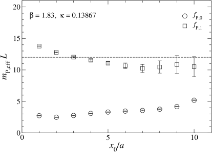
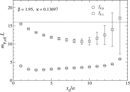
Figure 1: Effective mass $m_{\rm P,eff}=\frac{1}{2a}\log(f_{{\rm P},i}(x_{0}\!-\!a)/f_{{\rm P},i}(x_{0}\!+\!a))$ for $f_{\rm P,0}$ and $f_{\rm P,1}$ rescaled by $L$. The dotted line shows where the effective mass is equal to $a^{-1}$.

Note, however, that the effective mass $m_{{\rm P},1}$ at our smallest $\beta$ is already close to the cutoff (i.e. $m_{{\rm P},1}\,L\sim L/a$ in fig. 1). This implies that a rapid increase of the residual ${\rm O}(a^{2})$ effects might occur if one were to evaluate the improvement condition at even coarser lattice spacings.

4.2 The improvement coefficient

With the projected correlation functions we can proceed to the extraction of $c_{\rm A}$ itself. Table 3 lists the differences $\Delta r$ and $\Delta s$ for the lightest quark mass at each $\beta$. In all cases we see a good signal for $\Delta s$ and thus have a large sensitivity to $c_{\rm A}$.

$\beta$	$\kappa$	$a\,\Delta r$	$a^{2}\,\Delta s$	$L^{2}\,\Delta s$
1.83	0.13867	0.0229(14)	0.429(22)	62(3)
1.95	0.13697	0.0072(17)	0.236(14)	60(4)
2.05	0.13604	0.0036(13)	0.133(16)	53(2)

Table 3: Examples of $\Delta r$ and $\Delta s$ at $x_{0}\!=\!T/2$.

In fig. 2, we plot the effective $c_{\rm A}(x_{0})$, cf. eq. (14), from the finest and coarsest lattices. The value of $c_{\rm A}(x_{0})$ stabilizes after only a few lattice spacings from the lower temporal boundary where higher exited states contribute. In all cases $x_{0}=T/2$ is already in the region, where these effects are small and we use this choice to complete the definition of $c_{\rm A}$. Results for the improvement coefficient and the PCAC quark mass from all simulations are collected in table 4.

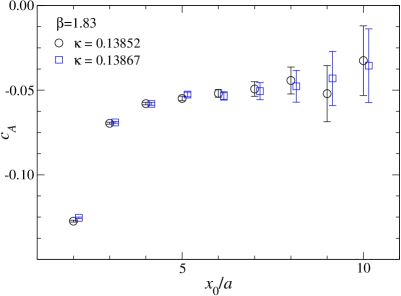
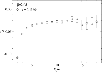
Figure 2: Effective value of $c_{\rm A}$ as a function of $x_{0}$ at $\beta\!=\!1.83$ (left panel) and $\beta\!=\!2.05$ (right panel). The data at $\beta\!=\!1.83$ and $\kappa\!=\!0.13867$ are slightly shifted along the vertical axis for clarity.

$\ \ \beta$	$\kappa$	$am$	$\quad\ c_{\rm A}$
2.05	0.13604	0.00554(14)	-0.0272(18)
1.95	0.13685	0.01020(29)	-0.0348(25)
	[interp.]	$am_{\rm ref}$	-0.0319(18)
	0.13697	0.00508(28)	-0.0303(24)
1.83	0.13852	0.01406(54)	-0.0519(23)
	[interp.]	$am_{\rm ref}$	-0.0528(17)
	0.13867	0.00614(63)	-0.0534(24)

Table 4: Numerical results for $am$ and $c_{\rm A}$. Also shown are the results of the interpolation to $m_{\rm ref}$ at the two coarser lattice spacings.

4.3 Interpolation of $c_{\rm A}$

As discussed above, we aim at evaluating the improvement condition on a line of constant physics in order to avoid potentially large O($a$) ambiguities in $c_{\rm A}$ itself. To this end we interpolate the results for $c_{\rm A}$ at $\beta=1.83$ and 1.95 to a quark mass $m_{\rm ref}$ that is matched to the one measured on the finest lattice. The quark mass dependence seems to be very small and thus the uncertainties in the quark masses become unimportant and we obtain $c_{\rm A}$ at $m_{\rm ref}$ with a small statistical error.

For future use we summarize the present results for the improvement coefficient in an interpolating formula (24), which by construction reduces to the one-loop result from refs. [38, 40] in the perturbative limit

$$c_{\rm A}(g_{0}^{2})=-0.0038\,g_{0}^{2}\,\times\,\frac{1-0.195\,g_{0}^{2}}{1-0.279\,g_{0}^{2}}\;.$$ (24)

It is plotted in fig 3, where one can verify that this formula reproduces the data well and gives a smooth interpolation in the range of $\beta$ values we simulated. As was the case with the plaquette gauge action and two quark flavors [33], the non–perturbative result is quite different from the one-loop estimate for practically relevant lattice spacings.

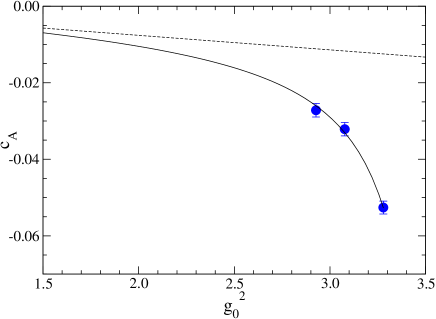
Figure 3: Non-perturbative estimate of $c_{\rm A}$ as a function of $g_{0}^{2}$.

4.4 Systematic uncertainties

The computation of $c_{\rm A}$ on a line of constant physics reduces the intrinsic ambiguity on the improvement coefficient to a smooth O($a$) form. Deviations from this condition will lead to systematic effects and we should therefore check the consequences of variations of the physical volume and quark mass for our improvement condition.

All simulations, on which we report here, are performed at fixed physical volume and we thus have no direct check of the volume effects on $c_{\rm A}$ from this improvement condition. From [33] we know that those can be large, but we know that our condition guarantees that they disappear smoothly as we approach the continuum limit, especially since our volume scaling is based on actual measurements of $r_{0}/a$.

From the data at the two coarser lattice spacings in table 4 it is evident that the quark mass dependence of $c_{\rm A}$ is very weak in our setup. This implies that no fine tuning of $m$ is required and also a posteriori justifies the fact that we ignore small changes of the renormalization factor in our range of $\beta$ and use the bare quark mass in our definition of a line of constant physics.

As mentioned above, the energy of the first excited state at our lowest $\beta\!=\!1.83$ is close to $a^{-1}$. Consequently, enforcing the present improvement condition at $\beta\!\lesssim\!1.83$ may induce large $O(a^{2})$ scaling violations in the axial current. While larger volumes might help in lowering this energy, the observation shows that even with improved gauge actions, one should not push the simulations too much towards coarse lattice spacings. On the other hand it is useful to repeat our earlier observation: within the range of lattice spacings covered here, we see a reasonable scaling of $L^{2}\,\Delta s$; this is a good hint that the considered matrix elements do not suffer from large $a$-effects. In retrospect the same statement can be made about the $N_{\rm f}=2$ computation with plaquette gauge action [33].

5 Conclusions

We have computed the O($a$)-improvement coefficient $c_{\rm A}(g_{0})$ of the axial current non-perturbatively in three-flavor QCD with the Iwasaki gauge action and non-perturbative $c_{\rm sw}(g_{0})$ [29]. The improvement coefficient $c_{\rm A}$ is parametrized as a function of $g_{0}$. Since the results connect smoothly to the one-loop formula at weak coupling, a simple interpolation formula (24) could be given in the range of $a^{-1}>1.6$ GeV.

We note that at the largest lattice spacing covered, the correction term amounts to 10 – 15% in decay constants $F_{\pi},\;F_{K}$ and then also in the renormalized quark masses evaluated from the PCAC relation. As a next step, a full non-perturbative evaluation of these quantities now requires the computation of the renormalization factor $Z_{\rm A}$ and for interesting applications of vector form factors also the corresponding quantities $Z_{\rm V}$ and $c_{\rm V}$ are very relevant. On the other hand, improvement terms proportional to the light quark masses are suppressed by the smallness of $am$. It then appears sufficient to approximate the associated coefficient by one-loop perturbation theory [38, 40].

References

- [1] L. Giusti, PoS LAT2006 (2006) 009, arXiv:hep-lat/0702014.
- [2] L. Del Debbio, L. Giusti, M. Lüscher, R. Petronzio and N. Tantalo, arXiv:hep-lat/0610059.
- [3] T. Ishikawa et al. (CP-PACS/JLQCD Collaborations), PoS LAT2006 (2006) 181, arXiv:hep-lat/0610050.
- [4] Y. Kuramashi et al., (PACS-CS Collaboration), PoS LAT2006 (2006) 029, arXiv:hep-lat/0610063.
- [5] S. R. Sharpe, PoS LAT2006 (2006) 022, arXiv:hep-lat/0610094.
- [6] C. Bernard et al., (MILC Collaboration), PoS LAT2006 (2006) 163, arXiv:hep-lat/0609053.
- [7] C. Allton et al., (RBC and UKQCD Collaborations), arXiv:hep-lat/0701013.
- [8] K. Jansen and C. Urbach (ETM Collaboration), arXiv:hep-lat/0610015.
- [9] Ph. Boucaud et al. (ETM Collaboration), arXiv:hep-lat/0701012.
- [10] H. Fukaya et al. (JLQCD Collaboration), arXiv:hep-lat/0702003.
- [11] K.G. Wilson, Phys. Rev. D10 (1974) 2445.
- [12] T. Reisz, Nucl. Phys. B318 (1989) 417.
- [13] M. Lüscher, Commun. Math. Phys. 54 (1977) 283.
- [14] M. Hasenbusch, Phys. Lett. B519 (2001) 177, arXiv:hep-lat/0107019.
- [15] S. Aoki et al. (JLQCD Collaboration), Phys. Rev. D65 (2002) 094507, arXiv:hep-lat/0112051
- [16] M. Lüscher, Comput. Phys. Commun. 165 (2005) 199, arXiv:hep-lat/0409106.
- [17] C. Urbach, K. Jansen, A. Shindler and U. Wenger, Comput. Phys. Commun. 174 (2006) 87, arXiv:hep-lat/0506011.
- [18] M. A. Clark and A. D. Kennedy, Phys. Rev. Lett. 98 (2007) 051601, arXiv:hep-lat/0608015.
- [19] L. Del Debbio, L. Giusti, M. Lüscher, R. Petronzio and N. Tantalo, JHEP 0602 (2006) 011, arXiv:hep-lat/0512021.
- [20] K. Symanzik, Nucl. Phys. B226 (1983) 187; ibid. Nucl. Phys. B226 (1983) 205.
- [21] B. Sheikholeslami and R. Wohlert, Nucl. Phys. B259 (1985) 572.
- [22] M. Lüscher, S. Sint, R. Sommer and P. Weisz, Nucl. Phys. B478 (1996) 365, arXiv:hep-lat/9605038.
- [23] M. Lüscher, Lectures given at the Les Houches Summer School “Probing the Standard Model of Particle Interactions”, Session LXVIII, 1997, R. Gupta, A. Morel, E. de Rafael and F. David eds. (Elsevier, Amsterdam), arXiv:hep-lat/9802029.
- [24] T. Bhattacharya, R. Gupta, W. Lee, S.R. Sharpe and J.M.S. Wu, Phys. Rev. D73 (2006) 034504, arXiv:hep-lat/0511014.
- [25] M. Lüscher, S. Sint, R. Sommer, P. Weisz and U. Wolff, Nucl. Phys. B491 (1997) 323, arXiv:hep-lat/9609035.
- [26] R. Sommer, arXiv:hep-lat/0611020.
- [27] K. Jansen and R. Sommer (ALPHA Collaboration), Nucl. Phys. B530 (1998) 185, arXiv: hep-lat/9803017.
- [28] N. Yamada et al. (CP-PACS/JLQCD Collaborations), Phys. Rev. D71 (2005) 054505, arXiv:hep-lat/0406028.
- [29] S. Aoki et al. (CP-PACS and JLQCD Collaborations), Phys. Rev. D73 (2006) 034501, arXiv:hep-lat/0508031.
- [30] T. Bhattacharya, R. Gupta, W.-J. Lee and S.R. Sharpe, Phys. Rev. D63 (2001) 074505, hep-lat/0009038.
- [31] S. Collins, C.T.H. Davies, G.P. Lepage and J. Shigemitsu (UKQCD Collaboration), Phys. Rev. D67 (2003) 014504, arXiv: hep-lat/0110159.
- [32] S. Dürr and M. Della Morte (ALPHA Collaboration), Nucl. Phys. B (Proc. Suppl.) 129 (2004) 417, arXiv:hep-lat/0309169.
- [33] M. Della Morte, R. Hoffmann and R. Sommer (ALPHA Collaboration), JHEP 0503 (2005) 029, arXiv:hep-lat/0503003.
- [34] M. Guagnelli et al. (ALPHA Collaboration), Nucl. Phys. B595 (2001) 44, arXiv:hep-lat/0009021.
- [35] Y. Iwasaki, Nucl. Phys. B258 (1985) 141; Univ. of Tsukuba report UTHEP-118 (1983), unpublished.
- [36] M .Lüscher, R. Narayanan, P. Weisz and U. Wolff, Nucl. Phys. B384 (1992) 168, arXiv:hep-lat/9207009.
- [37] S. Sint, Nucl. Phys. B421 (1994) 135, arXiv:hep-lat/9312079.
- [38] S. Aoki, R. Frezzotti and P. Weisz, Nucl. Phys. B540 (1999) 501, arXiv:hep-lat/9808007.
- [39] R. Sommer, Nucl. Phys. B411 (1994) 839, arXiv:hep-lat/9310022.
- [40] Y. Taniguchi and A. Ukawa, Phys. Rev. D58, (1998) 114503, arXiv:hep-lat/9806015.
- [41] S. Duane, A. D. Kennedy, B. J. Pendleton and D. Roweth, Phys. Lett. B195 (1987) 216.
- [42] T. Takaishi and P. de Forcrand, arXiv:hep-lat/0009024.
- [43] R. Frezzotti and K. Jansen, Nucl. Phys. B555 (1999) 395, arXiv:hep-lat/9808011.
- [44] A. D. Kennedy and J. Kuti, Phys. Rev. Lett. 54 (1985) 2473.
- [45] K. Jansen and C. Liu, Comput. Phys. Commun. 99 (1997) 221, arXiv:hep-lat/9603008.