Hadronic form factors in Lattice QCD at small and vanishing momentum transfer

Abstract:

The introduction of partially twisted boundary conditions allows weak and electromagnetic form factors to be evaluated at specified values of the hadronic momenta (and hence momentum transfers) in lattice simulations. We present and demonstrate this technique for the computation of the $K\to\pi$ semileptonic form factor at zero momentum transfer and for the electromagnetic form factor of the pion at arbitrarily small momentum transfers. These exploratory computations are carried out in full QCD with 3 flavours of sea quarks, but with only two values of $m_{u}=m_{d}$ which limits our ability to perform the chiral extrapolations. The results should therefore be viewed primarily as a demonstration of the feasibility of the method. For the $K\to\pi$ form factor we compare the new technique to the conventional approach and for the pion form factor we assess our results for very small momentum transfer with the help of chiral perturbation theory.

1 Introduction

In this paper we investigate the feasibility of using partially twisted boundary conditions in lattice computations to evaluate hadronic form factors at any chosen value of the momentum transfer. With conventional periodic boundary conditions on the quark fields on a spatial lattice of volume $L^{3}$ the components of the hadrons’ momenta are quantized to be integer multiples of $2\pi/L$ . This leads to a very poor momentum resolution for phenomenological studies. For example, on a $24^{3}$ lattice with lattice spacing $a\simeq 0.1$ fm, the components of the momentum are quantized in steps of about 0.5 GeV . The available momentum transfers are therefore also discrete. Using partially twisted boundary conditions we show that it is indeed possible to evaluate the form factors at any required momentum transfer, provided of course that the hadronic momenta are sufficiently small for lattice artefacts to be negligible. We illustrate the technique by evaluating:

1. the $K\to\pi$ form factors at zero $q^{2}$, where $q$ is the momentum transfer. These are required for the determination of the $V_{us}$ matrix element of the CKM matrix. In the standard approach to lattice computations of the $K\to\pi$ form factor at $q^{2}=0$, first proposed by Becirevic et al. [1, 2] and subsequently employed in a number of simulations [3, 4, 5, 6], the form factors are calculated (very precisely) at $q^{2}=q^{2}_{\textrm{max}}$ (corresponding to the pion and kaon both at rest) and somewhat less precisely at other accessible values of $q^{2}$. The results are then interpolated to $q^{2}=0$. In ref. [7], twisted boundary conditions were used in a quenched study to obtain the form factors at values of $q^{2}$ not accessible with periodic boundary conditions. In this paper we demonstrate that by using partially twisted boundary conditions in a dynamical simulation it is possible to evaluate the form factors directly at $q^{2}=0$ with comparable errors to the conventional approach but without the need for any interpolation in the momentum transfer, thus removing one source of systematic error [6].

2. the electromagnetic form factor of the pion at low momentum transfers (from which, for example, the charge radius can be determined). In particular we evaluate the form factor at values of $q^{2}$ below the minimum value obtainable with periodic boundary conditions; this minimum is given by $|q^{2}|=2m_{\pi}(m_{\pi}-\sqrt{m_{\pi}^{2}+(2\pi/L)^{2}})$. In contrast to recent lattice studies [8, 9, 10] this allows therefore for a direct evaluation of the charge radius of the pion.

These are two phenomenologically important examples, but we stress that the techniques can also be applied to a wide variety of hadronic matrix elements. The primary aim of this paper is to demonstrate the feasibility of the technique. We have therefore used a restricted set of quark masses and hence have only a very limited control of the chiral extrapolation. Having demonstrated the effectiveness of the technique we will now undertake a large-scale computation of the form factors.

The plan for the remainder of this paper is as follows. In the next section we introduce all the necessary definitions, correlation functions and ratios of correlation functions and then detail the new approaches to compute the $K_{l3}$ scalar and pion form factor. In particular, in section 2.3 we explain why it is possible to use a general set of partially twisted boundary conditions for the evaluation of the electromagnetic form factor of the pion. Section  3 contains the details of our numerical study together with the results and finally in section 4 we present a brief summary and outlook.

2 Description of the Technique

The matrix element of the vector current between initial and final states consisting of pseudoscalar mesons $P_{i}$ and $P_{f}$, respectively, is in general decomposed into two invariant form factors:

$$\langle P_{f}(p_{f})|V_{\mu}|P_{i}(p_{i})\rangle=f_{P_{i}P_{f}}^{+}(q^{2})(p_{i}+p_{f})_{\mu}+f_{P_{i}P_{f}}^{-}(q^{2})(p_{i}-p_{f})_{\mu}\,,$$ (1)

where $q=p_{i}-p_{f}$ is the momentum transfer. For $K\to\pi$ semileptonic decays $V_{\mu}$ is the weak current $\bar{s}\gamma_{\mu}u$, $P_{i}=K$ and $P_{f}=\pi$, whereas for the electromagnetic form factor of the pion $V_{\mu}$ is the electromagnetic current, both $P_{i}$ and $P_{f}$ are pions and vector current conservation implies that $f_{\pi\pi}^{-}(q^{2})=0$. The form factors $f_{P_{i}P_{f}}^{+}(q^{2})$ and $f_{P_{i}P_{f}}^{-}(q^{2})$ contain the non-perturbative QCD effects. In addition to the matrix elements considered here, form factors for other phenomenologically interesting semileptonic decays, for example for $B\to\pi$, $B\to D$ and $D\to K$ decays as well as those for decays into a vector final state, are also being computed in lattice simulations. As explained in the introduction, with the conventional periodic boundary conditions the form factors can only be evaluated at values of $q^{2}$ such that the components of momenta of the pseudoscalars, $\vec{p}_{i}$ and $\vec{p}_{f}$, are integer multiples of $2\pi/L$. Our aim is to compute the form factors at arbitrary preselected values of $q^{2}$ and in the following subsections we explain our technique for achieving this. We start with a brief introduction to twisted boundary conditions.

2.1 Twisted Boundary Conditions

It is well known that the choice of boundary conditions for particles or fields in quantum mechanics or field theory in a finite volume governs the momentum spectrum. This observation has been exploited in many applications. More recently it has been appreciated that by varying the boundary conditions the momentum resolution for lattice phenomenology can be significantly improved [11, 12, 13, 14, 15, 16, 7, 17, 18, 19]. However, if a new simulation (i.e. a new set of gauge configurations) were necessary for every choice of momentum, the use of twisted boundary conditions would be prohibitively expensive in computing resources and therefore impracticable. In ref. [13] it was demonstrated that for processes without final state interactions, such as the form factors studied in this paper, it is sufficient to apply twisted boundary conditions only on the valence quarks, whilst using sea quarks defined with periodic boundary conditions (see also ref.[14]). In this way the need for new simulations is avoided and the method becomes practicable. The introduction of such partially twisted boundary conditions changes the finite-volume corrections, but, as demonstrated in refs. [13, 20], they remain exponentially small in the volume and, as is standard, we neglect them.

In our study we use partially twisted boundary conditions, combining gauge field configurations generated with sea quarks with periodic boundary conditions with valence quarks with twisted boundary conditions, i.e. the valence quarks satisfy

$$\psi(x_{k}+L)=e^{i\theta_{k}}\psi(x_{k}),\qquad(k=1,2,3)\,,$$ (2)

where $\psi$ is either a strange quark $s$ or a light quark $q$. By varying $\vec{\theta}$ we can tune the momenta of the mesons continuously. For the purposes of our study it will be sufficient to twist only the valence quark in each meson, with the valence antiquark satisfying periodic boundary conditions (the generalization to antiquarks with twisted boundary conditions is also straightforward). The dispersion relation for the mesons is then

$$E=\sqrt{m^{2}+(\vec{p}_{\rm FT}+\vec{\theta}/L)^{2}},$$ (3)

where $m$ is the mass of the meson and $\vec{p}_{\rm FT}$ is the meson momentum induced by Fourier summation (the components of $\vec{p}_{\rm FT}$ are integer multiples of $2\pi/L$).

For the matrix element in (1) with the initial and the final meson carrying momenta $\vec{p}_{i}$ and $\vec{p}_{f}$, respectively, the momentum transfer between the initial and the final state meson is

$$q^{2}=(p_{i}-p_{f})^{2}=\left\{[E_{i}(\vec{p}_{i})-E_{f}(\vec{p}_{f})]^{2}-\left[(\vec{p}_{{\rm FT},i}+\vec{\theta}_{i}/L)-(\vec{p}_{{\rm FT},f}+\vec{\theta}_{f}/L)\right]^{2}\right\}.$$ (4)

2.2 Correlation Functions

In order to determine the form factors we compute two- and three-point correlation functions. The two-point function is defined by

$$C_{i}(t,\vec{p}_{i})=\sum_{\vec{x}}e^{i\vec{p}_{i}\cdot\vec{x}}\langle\,O_{i}(t,\vec{x})\,O_{i}^{\dagger}(0,\vec{0})\,\rangle=\frac{|Z_{i}|^{2}}{2E_{i}}\left(e^{-E_{i}t}+e^{-E_{i}(T-t)}\right)\,,$$ (5)

where $i=\pi$ or $K$, the $O_{i}$ are local pseudoscalar interpolating operators for the corresponding mesons $O_{\pi}=\bar{q}\gamma_{5}q$ and $O_{K}=\bar{s}\gamma_{5}q$ and we assume that $t$ and $T-t$ (where $T$ is the temporal extent of the lattice) are sufficiently large that the correlation function is dominated by the lightest state (i.e. the pion or kaon). The constants $Z_{i}$ are given by $Z_{i}=\langle\,P_{i}\,|\,O_{i}^{\dagger}(0,\vec{0})\,|\,0\,\rangle$ . The three-point functions are defined by

$$C_{P_{i}P_{f}}(t_{i},t,t_{f},\vec{p}_{i},\vec{p}_{f}) = \sum_{\vec{x}_{f},\vec{x}}e^{i\vec{p}_{f}\cdot(\vec{x}_{f}-\vec{x})}e^{i\vec{p}_{i}\cdot\vec{x}}\langle\,O_{f}(t_{f},\vec{x}_{f})\,V_{4}(t,\vec{x})\,O_{i}^{\dagger}(t_{i},\vec{0})\,\rangle$$ (6)

$$= \frac{Z_{i}\,Z_{f}}{4E_{i}E_{f}}\,\langle\,P_{f}(\vec{p}_{f})\,|\,V_{4}(0)\,|\,P_{i}(\vec{p}_{i})\,\rangle\,$$

$$\times\left\{\theta(t_{f}-t)\,e^{-E_{i}(t-t_{i})-E_{f}(t_{f}-t)}\ -\ \theta(t-t_{f})\,e^{-E_{i}(T+t_{i}-t)-E_{f}(t-t_{f})}\right\}\,,$$

where $P_{i,f}$ is a pion or a kaon and $V_{4}$ is the time component of the vector current with flavour quantum numbers to allow the $P_{i}\to P_{f}$ transition and where we have defined $Z_{f}=\langle\,0\,|\,O_{f}(0,\vec{0})|\,P_{f}\,\rangle$. Again we assume that all the time intervals are sufficiently large for the lightest hadrons to give the dominant contribution. For the remainder of this paper we choose to keep $t_{i}$ and $t_{f}$ fixed (with $t_{i}=0$ and $t_{f}=T/2$) and we will therefore only explicitly refer to them where necessary  and write $C_{P_{i}P_{f}}(t,\vec{p}_{i},\vec{p}_{f})$ with just three arguments.

The correctly normalized vector currents $V_{\mu}$ in eq. (6) are obtained by multiplying the local currents used in the numerical simulations by the normalization constant $Z_{V}$ defined by

$$Z_{V}=\frac{1}{2}\frac{C_{\pi}(t_{f}=T/2,0)}{C^{B}_{\pi\pi}(t,0,0)},$$ (7)

where the index $B$ in $C^{B}_{\pi\pi}(t,0,0)$ implies that the bare vector current is being used. The factor of $\frac{1}{2}$ in eq. (7) corresponds to the two terms on the right hand side of eq. (5).

In order to extract the matrix element $\langle\,P_{f}(\vec{p}_{f})\,|\,V_{4}(0)\,|\,P_{i}(\vec{p}_{i})\,\rangle$ effectively, it is convenient to define the three ratios:

$$\begin{array}[]{rcl}R_{1,\,P_{i}P_{f}}(\vec{p}_{i},\vec{p}_{f})&{=}&4\sqrt{E_{i}E_{f}}\,\sqrt{\frac{C_{P_{i}P_{f}}(t,\vec{p}_{i},\vec{p}_{f})\,C_{P_{f}P_{i}}(t,\vec{p}_{f},\vec{p}_{i})}{C_{P_{i}}(T/2,\vec{p}_{i})\,C_{P_{f}}(T/2,\vec{p}_{f})}},\\[11.38109pt] R_{2,\,P_{i}P_{f}}(\vec{p}_{i},\vec{p}_{f})&=&2\sqrt{{E_{i}E_{f}}}\,\sqrt{\frac{C_{P_{i}P_{f}}(t,\vec{p}_{i},\vec{p}_{f})\,C_{P_{f}P_{i}}(t,\vec{p}_{f},\vec{p}_{i})}{C_{P_{i}P_{i}}(t,\vec{p}_{i},\vec{p}_{i})\,C_{P_{f}P_{f}}(t,\vec{p}_{f},\vec{p}_{f})}},\\[11.38109pt] R_{3,\,P_{i}P_{f}}(\vec{p}_{i},\vec{p}_{f})&=&4{\sqrt{E_{i}E_{f}}}\,\frac{C_{P_{i}P_{f}}(t,\vec{p}_{i},\vec{p}_{f})}{C_{P_{f}}(T/2,\vec{p}_{f})}\,\sqrt{\frac{C_{P_{i}}(T/2-t,\vec{p}_{i})\,C_{P_{f}}(t,\vec{p}_{f})\,C_{P_{f}}(T/2,\vec{p}_{f})}{C_{P_{f}}(T/2-t,\vec{p}_{f})\,C_{P_{i}}(t,\vec{p}_{i})\,C_{P_{i}}(T/2,\vec{p}_{i})}}\,.\end{array}$$ (8)

For sufficiently large $t$ and $T/2-t$, so that only the lightest mesons contribute significantly to each of the correlation functions, each of the three ratios is independent of $t$ and is equal to the matrix element $\langle\,P_{f}(\vec{p}_{f})\,|\,V_{4}(0)\,|\,P_{i}(\vec{p}_{i})\,\rangle$. Here we are assuming that $t$ is in the forward half of the lattice $0<t<T/2$. The correlation functions for $t$ in the backward half, $T/2<t<T$ are readily related to those in the forward half and hence can be combined with them to construct the ratios in (8). We discuss the quality of the plateaus and the numerical determination of the form factors in section 3.

2.3 The Pion’s Form Factor with Twisted Boundary Conditions

A sketch of the quark-flow diagram for the transition in eq. (1), with the final-state meson $P_{f}$ composed of valence quarks ($q_{1}\bar{q}_{3}$) and the initial-state meson with valence quarks ($q_{2}\bar{q}_{3}$) is as follows:

For $K_{\ell 3}$ decays, specifically for the decay $\bar{K}^{0}\to\pi^{+}\ell\nu_{l}$, each of the three valence has a different flavour, $q_{1}=u,\,q_{2}=s$ and $q_{3}=d$, and the partially twisted theory can be readily constructed as discussed in ref. [13]. We can therefore introduce three independent twisting angles for the three flavours. For the electromagnetic form factor of the pion however, $q_{1}$ has the same flavour as $q_{2}$, nevertheless it is still possible to use partially twisted boundary conditions to evaluate the form factor, with three different twisting angles for the three valence quarks, as we now explain .

1. We start by imagining that we evaluate the matrix element $\langle\pi(p_{f})\,|\,V_{\mu}\,|\,\pi(p_{i})\rangle$ in an infinite volume in full QCD with 3 flavours of sea quarks. We assume isospin symmetry, and it will be important to note that in this case $G$-parity implies that only the isovector component of the electromagnetic current couples to pions. When we consider partially quenched QCD below, this will imply that the vector current is composed of valence quark fields.

2. We next consider the partially quenched 3-flavour theory in which $m_{u}^{V}=m_{d}^{V}=m_{u}^{S}=m_{d}^{S}=m_{s}^{V}$, where the superscripts $V$ and $S$ label valence and sea, respectively, and $m_{s}^{S}$ is equal to the physical strange quark mass. The partial quenching arises because the mass of the valence strange quark is different to that of the sea strange quark. However, since the valence strange quark plays no role in the evaluation of $\langle\pi(p_{f})\,|\,V_{\mu}\,|\,\pi(p_{i})\rangle$, this matrix element is correctly given in this theory.

3. We now exploit the $SU(3)$ flavour symmetry in the valence sector which implies that, for example,

   $$\langle\pi^{+}(p_{f})\,|\,\bar{u}\gamma^{\mu}u\,|\,\pi^{+}(p_{i})\rangle=-\langle\pi^{+}(p_{f})\,|\,\bar{d}\gamma^{\mu}d\,|\,\pi^{+}(p_{i})\rangle=\langle\pi^{+}(p_{f})\,|\,\bar{u}\gamma^{\mu}s\,|\,\bar{K}^{0}(p_{i})\rangle\,,$$ (9)

   where the fields in the currents correspond to valence quarks. The pion’s form factor in this partially quenched theory is therefore equal to that of the $K\to\pi$ transition (the degeneracy of the three flavours of valence quark implies that there is now also only a single form factor also for $K\to\pi$ transitions).

   Up to this point we have not made any approximations. For example, the $SU(3)$ flavour symmetry in the valence sector implies that exactly the same diagrams arise in chiral perturbation theory ($\chi$PT) in the evaluation of the matrix element$\langle\pi^{+}(p_{f})\,|\,\bar{u}\gamma^{\mu}s\,|\,\bar{K}^{0}(p_{i})\rangle$ in the partially quenched theory as for $\langle\pi(p_{f})\,|\,V_{\mu}\,|\,\pi(p_{i})\rangle$. Of course the labelling of the quark content of the mesons may be different; in one case we may have a meson with a strange valence quark and in the other an $u$-quark, but as they are degenerate the diagrams give identical contributions (as they must by symmetry). In particular, in contrast to the general case for partially quenched theories, there are no hairpin contributions here.

4. Finally we consider performing the simulations in finite volume, taking all the sea quarks to have periodic boundary conditions. For the three flavours of valence quarks however, we introduce different twists, $\vec{\theta}_{u},\,\vec{\theta}_{d}$ and $\vec{\theta}_{s}$, which changes the momentum spectrum but not the mass spectrum. For propagators in $\chi$PT with quark content of the form $\bar{q}q\ (q=u^{V},d^{V},s^{V})$, the effects of the twisted boundary condition cancel and the spectrum is the same as for the mesons composed of the corresponding sea quarks (i.e. as if the boundary conditions were periodic). Thus, in spite of the different masses of the valence and sea strange quarks, no double-pole hairpin contributions are introduced.

   For valence flavour non-singlet mesons, the momentum spectrum is changed by using twisted boundary conditions rather than periodic ones. However, as explicitly demonstrated in Appendix A of ref. [13], at one-loop order in $\chi$PT the resulting summations in finite-volume are equal to the corresponding infinite volume integrals, up to exponentially small terms in the volume. Such exponentially small terms are also present with periodic boundary conditions and are generally neglected.

We have therefore established that we can evaluate the pion form factor with 3 different twisting angles for the valence quarks (up to the usual exponential precision in the volume).

2.4 $f^{+}_{K\pi}(0)$ and $f_{\pi\pi}(q^{2})$ at Small Momentum Transfers

We wish to compute the scalar form factor for $K_{\ell 3}$ decays at zero momentum transfer, $f^{0}_{K\pi}(0)$. The scalar form factor is defined in terms of $f^{+}_{K\pi}$ and $f^{-}_{K\pi}$ by:

$$f_{K\pi}^{0}(q^{2})=f_{K\pi}^{+}(q^{2})+{q^{2}\over m_{K}^{2}-m_{\pi}^{2}}f_{K\pi}^{-}(q^{2}),$$ (10)

and $f^{0}_{K\pi}(0)=f_{K\pi}^{+}(0)$.

Our approach is to use twisted boundary conditions to induce momenta for the pion and kaon such that $q^{2}=0$. A simple way to do this is to take the pion (kaon) to be at rest and to tune the momentum of the kaon (pion). We therefore compute the ratios

$$\begin{array}[]{llcccc}&R_{\alpha,K\pi}(\vec{p}_{K},\vec{0})&\textrm{with}&|\vec{\theta}_{K}|=L\sqrt{({m_{K}^{2}+m_{\pi}^{2}\over 2m_{\pi}})^{2}-m_{K}^{2}}&\textrm{and}&\vec{\theta}_{\pi}=\vec{0}\\[5.69054pt] {\rm and}&R_{\alpha,K\pi}(\vec{0},\vec{p}_{\pi})&\textrm{with}&|\vec{\theta}_{\pi}|=L\sqrt{({m_{K}^{2}+m_{\pi}^{2}\over 2m_{K}})^{2}-m_{\pi}^{2}}&\textrm{and}&\vec{\theta}_{K}=\vec{0}\,,\\[5.69054pt] \end{array}$$ (11)

where $\alpha=1,2,3$. The momenta of the mesons are given by $\vec{p}_{K}=\vec{\theta}_{K}/L$ and $\vec{p}_{\pi}=\vec{\theta}_{\pi}/L$ and it can be readily verified that the choices of twisting angles in the two lines of eq.(11) both correspond to $q^{2}=0$.

The required form factor, $f^{0}_{K\pi}(0)$, can be obtained directly from a linear combination of the ratios in eq. (11):

$$f_{K\pi}^{0}(0)=\frac{R_{\alpha,K\pi}(\vec{p}_{K},\vec{0})(m_{K}-E_{\pi})-R_{\alpha,K\pi}(\vec{0},\vec{p}_{\pi})(E_{K}-m_{\pi})}{(E_{K}+m_{\pi})(m_{K}-E_{\pi})-(m_{K}+E_{\pi})(E_{K}-m_{\pi})}\qquad(\alpha=1,2,3)\,.$$ (12)

Here $E_{K}$ ($E_{\pi}$) is the energy of the kaon (pion) corresponding to the momentum induced by the twisting angle in the first (second) line of eq.(11).

By using the spatial component of the vector current $V_{k}$ ($k=1,2$ or 3) it is possible to tune the momenta such that $q^{2}=0$ and $q_{k}=0$ so that one obtains the form-factor $f^{+}(0)$ directly. We find however, that this procedure leads to a significantly larger statistical error.

The case of the pion’s electromagnetic form factor is simpler since current conservation implies that $f_{\pi\pi}^{-}(q^{2})=0$ so that (dropping the redundant superscript $+$)

$$\langle\pi^{+}(p_{f})|V_{\mu}(0)|\pi^{+}(p_{i})\rangle=f_{\pi\pi}(q^{2})\,(p_{i}+p_{f})_{\mu}.$$ (13)

$f_{\pi\pi}(q^{2})$ can therefore be directly computed from the ratios in eq.(8) by inducing the required momenta for the initial- and final-state pions.

2.5 Comparison with the Conventional Approaches

One aim of this paper is to compare the precision with which we can determine the form factors using the techniques introduced in the preceding subsection with that obtained using standard methods. The numerical comparison will be given in section 3, here we describe what the conventional approaches are.

Recent calculations of $f^{0}_{K\pi}(0)$ follow the procedure introduced by Becirevic et al. [1]. The scalar form factor at $q^{2}=0$ is determined using a phenomenologically motivated interpolation of $f^{0}_{K\pi}(q^{2})$ between the point at $q^{2}_{\rm max}=(m_{K}-m_{\pi})^{2}$ and points at negative values of $q^{2}$ which are accessible by Fourier summation with periodic boundary conditions. The value of $f^{0}_{K\pi}(q^{2}_{\rm max})$ is readily obtained with excellent statistical precision from

$$R_{2;K\pi}(\vec{0},\vec{0})=f_{K\pi}^{0}(q^{2}_{\rm max})(m_{K}+m_{\pi})\,.$$ (14)

The interpolation in $q^{2}$ (to $q^{2}=0$) is constrained by computing $f_{K\pi}^{+}(q^{2})$ and $f_{K\pi}^{-}(q^{2})$ (and hence $f_{K\pi}^{0}(q^{2})$) for a variety of values of $q^{2}$. In order to improve precision, where possible ratios of correlation functions are used. $f_{K\pi}^{+}(q^{2})$ and $f_{K\pi}^{-}(q^{2})$ can be written in the form

$$f_{K\pi}^{+}(q^{2})={F(p_{K},p_{\pi})}f_{K\pi}^{0}(q^{2}_{\rm max})\left(1+{E_{K}({\vec{p}}_{K})-E_{\pi}({\vec{p}}_{\pi})\over E_{K}({\vec{p}}_{K})+E_{\pi}({\vec{p}}_{\pi})}{\xi(q^{2})}\right)^{-1},$$ (15)

and

$$f_{K\pi}^{-}(q^{2})=f_{K\pi}^{+}(q^{2}){\xi(q^{2})}.$$ (16)

In order to define the quantities $F(p,p^{\prime})$ and $\xi(q^{2})$ used in these expressions we start by defining the ratio of correlation functions

$$\tilde{R}_{k}(\vec{p}_{K},\vec{p}_{\pi})=\frac{C_{k,\,K\pi}(t,{\vec{p}}_{K},{\vec{p}}_{\pi})\,C_{KK}(t,{\vec{p}}_{K},{\vec{p}}_{\pi})}{C_{K\pi}(t,{\vec{p}}_{K},{\vec{p}}_{\pi})\,C_{k,\,KK}(t,{\vec{p}}_{K},{\vec{p}}_{\pi})}\,,$$ (17)

where $k=1,2,3$ is a spatial index and $C_{k,\,P_{i}P_{f}}(t,{\vec{p}}_{i},{\vec{p}}_{f})$ is the three point correlation function defined in eq. (6) with $V_{4}$ replaced by $V_{k}$ . For time intervals such that only the lightest states contribute significantly, $\tilde{R}_{k}$ is independent of $t$. $\xi$ and $F$ are then defined by:

$$\xi(q^{2})=\frac{-\left(E_{K}({\vec{p}}_{K})+E_{K}({\vec{p}}_{\pi})\right)\left(p_{K}+p_{\pi}\right)_{k}+\left(E_{K}({\vec{p}}_{K})+E_{\pi}({\vec{p}}_{\pi})\right)\left(p_{K}+p_{\pi}\right)_{k}\tilde{R}_{k}(\vec{p}_{K},\vec{p}_{\pi})}{\hskip 11.38109pt\left(E_{K}({\vec{p}}_{K})+E_{K}({\vec{p}}_{\pi})\right)\left(p_{K}-p_{\pi}\right)_{k}-\left(E_{K}({\vec{p}}_{K})-E_{\pi}({\vec{p}}_{\pi})\right)\left(p_{K}+p_{\pi}\right)_{k}\tilde{R}_{k}(\vec{p}_{K},\vec{p}_{\pi})},$$ (18)

and

$$\frac{C_{K\pi}(t,{\vec{p}}_{K},{\vec{p}}_{\pi})\,C_{K}(t,{\vec{0}})\,C_{\pi}(T/2-t,{\vec{0}})}{C_{K\pi}(t,{\vec{0}},{\vec{0}})\,C_{K}(t,{\vec{p}}_{K})\,C_{\pi}(T/2-t,{\vec{p}}_{\pi})}=\frac{E_{K}({\vec{p}}_{K})+E_{\pi}({\vec{p}}_{\pi})}{m_{K}+m_{\pi}}F(p_{K},p_{\pi})\,.$$ (19)

Having determined $f_{K\pi}^{+}(q^{2})$ and $f_{K\pi}^{-}(q^{2})$ for a variety of values of $q^{2}<0$ and at $q^{2}_{\textrm{max}}$, we fit the results to some ansatz for the $q^{2}$ behaviour and determine the scalar form factor at $q^{2}=0$. It should be noted that in addition to the systematic uncertainties introduced by the choice of ansatz, one is limited to the number of values of $q^{2}$ one can use while keeping the lattice artefacts small enough for the required precision.

Recent examples for the use of this approach have been presented in refs. [3, 4, 5, 6].

3 Results for the Form Factors

In this section we describe the details of our numerical simulation and present our results.

3.1 Lattice Parameters

For the numerical studies presented in this paper we use two ensembles out of the set of $N_{f}=2+1$ flavour Domain Wall Fermion [21, 22, 23] configurations with $(L/a)^{3}\times T/a\times L_{s}=16^{3}\times 32\times 8$ which were jointly generated by the UKQCD/RBC collaborations using the QCDOC computer [24, 25, 26, 27]. A detailed study of the light-hadron spectrum and other hadronic quantities using these configurations has recently been reported in ref. [28]. In particular, we use the gauge configurations generated with the DBW2 gauge action [29, 30] at $\beta=0.72$. The bare strange quark mass is $am_{s}=0.04$ and we use two different ensembles with light quark masses $am_{l}=0.02$ and $am_{l}=0.01$ respectively. The corresponding pion and kaon masses are summarized in table 1 and for the inverse lattice spacing we take $a^{-1}=1.6(1)$ GeV. We use the jackknife technique to estimate the statistical errors.

We generate the three point functions of type (6) by contracting propagators $S(t,\vec{x};t_{i},\vec{0})$ from the origin to any point $(t,\vec{x})$ with the generalized quark propagator [31] defined by

$$S^{\prime}(t_{i},\vec{0};t_{f},\vec{p}_{f};t,\vec{x})=\sum_{\vec{x}_{f}}\gamma_{5}\left(S(t,\vec{x};t_{f},\vec{x}_{f})\gamma^{5}S(t_{f},\vec{x}_{f};t_{i},\vec{0})\,e^{-i\vec{p}_{f}\cdot\vec{x}_{f}}\right)^{\dagger}\gamma_{5}\,,$$ (20)

where we suppress the label indicating the twisting angle on the propagators (cf. fig. 1).

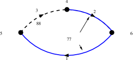
Figure 1: The three point function $C_{P_{i}P_{f}}(t_{i},t,t_{f},\vec{p}_{i},\vec{p}_{f})$ defined in (6) in terms of the the quark propagator $S(t,\vec{x};t_{i},\vec{0})$ (dashed black) and the generalized quark propagator $S^{\prime}(t_{i},\vec{0};t_{f},\vec{p};t,\vec{x})$ (solid blue).

For the present study we generate the generalized propagators in (20) with $\vec{p}_{f}=0$, although it would be straightforward to extend the study to include other values.

For the $K_{\ell 3}$ form factors in all cases one meson is at rest and the other has a momentum which is induced entirely by the twisted boundary conditions. As a result we can evaluate all three ratios $R_{\alpha,K\pi}(\vec{p}_{K},\vec{p}_{\pi})$ at a comparable computational cost. A selection of the plateaus for the $K_{l3}$ decay is presented for illustration in fig. 2. We find that, for the choice of parameters used in this study, ratio $R_{1,K\pi}(\vec{p}_{K},\vec{p}_{\pi})$ and $R_{2,K\pi}(\vec{p}_{K},\vec{p}_{\pi})$ have the most pronounced plateaus and the fits lead to comparable final statistical errors. The results we present in the following have been obtained from fits to $R_{1,K\pi}(\vec{p}_{K},\vec{p}_{\pi})$.

For the electromagnetic form factor of the pion we allow one of the pions to have a non-zero value of Fourier momentum (i.e. its momentum is given by $(2\pi\,\vec{n}+\vec{\theta})/L$, where $\vec{n}$ is a vector of integers and $\vec{\theta}$ is the vector of twisting angles). In order to evaluate the ratios $R_{1,\pi_{i}\pi_{f}}(\vec{p}_{\pi_{i}},\vec{p}_{\pi_{f}})$ and $R_{2,\pi_{i}\pi_{f}}(\vec{p}_{\pi_{i}},\vec{p}_{\pi_{f}})$ we would require the generalized propagators in (20) at non-zero $\vec{p}$ and here we restrict our computations to the evaluation of $R_{3,\pi_{i}\pi_{f}}(\vec{p}_{\pi_{i}},\vec{p}_{\pi_{f}})$. A typical result for this ratio is illustrated in fig. 3.

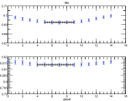
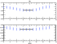
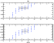
Figure 2: Examples of results for the three different ratios defined in (8) for the $K_{l3}$ decay. The two rows correspond to the two quark masses $am_{l}=0.01$ (upper row) and $am_{l}=0.02$ (lower row), respectively. In each case the kaon is at rest and the pion has a momentum induced by the twisting angle.

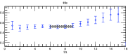
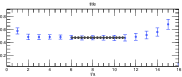
Figure 3: Example of a typical result for $R_{3}$ (cf. eq. (8)) for the pion form factor for $am_{l}=0.01$ (left) and $am_{l}=0.02$ (right). Here the source momentum is $|ap|=0.39$ and the sink momentum is $0.1$.

3.2 The $K\to\pi$ Form Factor, $f^{+}_{K\pi}(0)$

We computed the $K_{\ell 3}$-form factor using both the conventional and our new approach for two values of the light quark mass on 200 configurations with a separation of 10 trajectories. The conventional approach has been described in section 2.5 above; for more details on the analysis see refs. [1, 4, 5]. For this conventional calculation, we average all correlation functions over results from two positions of the propagator source, $(0,0,0,0)$ and $(8,8,8,16)$. For the new approach we generate correlation functions using only a single source, (0,0,0,0), but averaging over three equivalent twisting angles, i.e. $\vec{\theta}_{i}=(\theta_{i},0,0)$, $(0,\theta_{i},0)$ or $(0,0,\theta_{i})$, with $i=\pi$ or $K$. The numerical values of $\theta_{\pi}$ and $\theta_{K}$ obtained using eq. (11) are presented in table 1.

In order to choose the twisting angles which correspond to $q^{2}=0$ using equation (11) we need to know what the masses of the mesons are. We initially estimated these using a subset of 100 configurations from the same ensembles and using only one position for the source of the propagator. The mean values obtained in this way are $am_{\pi}^{0.01}=0.306$, $am_{K}^{0.01}=0.399$, $am_{\pi}^{0.02}=0.374$ and $am_{K}^{0.02}=0.430$, to be compared with those eventually determined on the full ensemble and averaged over various positions of the propagator source given in table 1. The small differences in the central values, together with discretization effects in the pion and kaon dispersion relation lead to a small deviation in $q^{2}$ from 0. We summarize this effect in table 1 where the quoted values for $q^{2}$ are obtained using eq. (4) with the corresponding meson energies determined from fits to the respective two point correlation function.

We present our results in the plots in fig. 4. The left-hand plot shows the data points which one obtains from correlation functions with one meson at rest and the other with momentum of magnitude $\,|\vec{p}\,|=0,{2\pi/L}$ or $\sqrt{2}\,(2\pi/L)$. Since in addition to $f_{K\pi}^{0}(q^{2})$ we also compute $f^{0}_{\pi K}(q^{2})$, from equations (15)-(19) (modified in the obvious way) we obtain results for the form factor at four additional values of $q^{2}$ for each value of the quark mass.

		$am_{l}=0.02$	$am_{l}=0.01$
	$am_{\pi}$	0.3765(21)	0.3002(23)
	$am_{K}$	0.4312(20)	0.3942(20)
$f_{K\pi}$	${\theta}_{\pi}$	0.838	1.315
	${\theta}_{K}$	0.963	1.714
	$q^{2}_{\rm max}$	0.00299(5)	0.00883(20)
	$q^{2}_{\theta_{\pi}}$	-0.00012(4)	0.00016(17)
	$q^{2}_{\theta_{K}}$	-0.00017(5)	0.00017(23)
$f_{\pi\pi}$	${\theta}_{\pi}$	0, 1.6, 2.3	0, 1.6, 2.3

Table 1: Summary of kinematical parameters for the studies involving twisted boundary conditions.

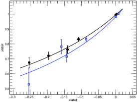
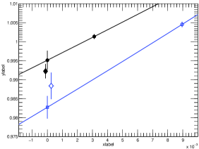
Figure 4: Results for the form factor ($am_{l}=0.02$ as full black circles and $am_{l}=0.01$ as blue squares). Left: All data points entering the conventional approach. Right: Zoom which shows the data points for both the new (diamonds) and the conventional approach at $q^{2}=0$ and the data points at $q^{2}_{\rm max}$.

The corresponding values of $q^{2}$ are determined by using the pion and kaon masses obtained from fits to two-point functions as input to the continuum dispersion relation. The curves represent a fit using the pole-dominance ansatz

$$f^{0}_{K\pi}(q^{2})=\frac{f_{K\pi}^{0}(0)}{1-q^{2}/M^{2}}\,,$$ (21)

where $M$ is a parameter fitted from the data.

The right-hand plot shows a zoom into the region around $q^{2}=0$. The two data points at $q^{2}>0$ correspond to the results for $q^{2}_{\rm max}$ for which the pion and kaon are both at rest; they can be identified by their strikingly small errors. We also display the results for $f_{K\pi}^{0}(q^{2}=0)$ obtained from the pole fit (21) at each quark mass. In addition the right plot of fig. 4 contains the results from the new approach.

We obtain the following results using the conventional and the new approach:

	$am_{l}$	0.02	0.01
$f_{K\pi}^{0}(0)$	conventional	0.9951(24)	0.9827(29)
	new	0.9926(34)	0.9884(34)

The results for $f_{K\pi}(0)$ as determined from the conventional and the new approaches do not agree exactly but the discrepancy is statistically not significant. The size of the statistical errors is similar in the two approaches, which is an important condition for establishing the new technique. The main motivation for the direct approach advocated in this paper is to avoid the need for an ansatz with which to perform the $q^{2}$ interpolation and this is apparently achieved without significantly inflating the error. In addition, it should be stressed that the points at negative $q^{2}$ are obtained with $|\,\vec{p}\,|=2\pi/L$ and $\,|\vec{p}\,|=\sqrt{2}\,2\pi/L$, so that with $L/a=16$ one may have concerns about the size of the lattice artefacts at these momenta. Our results show that both concerns can now be eliminated by using the new approach.

As stated in the introduction, this is an exploratory study in which we investigate the feasibility of the method rather than aim for the ultimate physical results. In particular it will be important to check the precision of the direct approach as the mass of the light quark is reduced and/or the volume is increased. Reducing the light quark mass leads to an increase of $q^{2}_{\rm max}$ and therefore the value for the form factor $f_{K\pi}(0)$ will be more susceptible to the choice for the interpolation in $q^{2}$ in the conventional approach. Simulating in larger volumes, in addition to reducing the finite-volume corrections, enables smaller Fourier momenta (with components which are integer multiples of $2\pi/L$) to be reached, so that the data points at non-vanishing momentum in the conventional approach move closer to $q^{2}=0$ and thus better constrain the interpolation.

3.3 The Electromagnetic Form Factor of the Pion, $f_{\pi\pi}(q^{2})$

We compute the pion’s electromagnetic form factor for two values of the light quark mass $am_{l}=0.02$ and $am_{l}=0.01$ on 200 configurations separated by 10 trajectories in Monte Carlo time. We generate pion three-point functions $C_{\pi\pi}$ with all possible mutual combinations of the twisting angles $\theta_{1,2}$ as given in table 1 (cf. also fig. 1), with the twist being applied only in one direction (i.e. $\vec{\theta}_{1,2}=(\theta_{1,2},0,0)$). After projecting on the Fourier momenta of magnitudes $|\vec{p}_{\rm FT}|=0,$ $2\pi/L,$ and $\sqrt{2}\,(2\pi/L)$ for the initial state, we are thus able to generate data points for the form factor in the entire range from $q^{2}=0$ to approximately $1\,{\rm GeV}^{2}$. We average the results obtained for degenerate values of $q^{2}$ (see eq. (4) ). A simplification compared to the $K_{\ell 3}$ scalar form factor is that we do not need $Z_{V}$; current conservation implies that $f_{\pi\pi}(0)=1$ and this provides the required normalization.

As was noted in ref. [10], for large values of the initial and/or final pion’s momentum the argument of the square root in $R_{3}$ may become negative due to statistical fluctuations. To avoid this problem we follow ref. [10] and consider the two-point functions at smaller times, making the replacement,

$$C_{\pi}(T/2,\vec{p})\to\frac{C_{\pi}(T/2-t_{\rm shift},\vec{p})}{\cosh(E_{\pi}(\vec{p})t_{\rm shift})},$$ (22)

and we find that $t_{\rm shift}/a=7$ gives the best results. This removes the occurrence of negative arguments in the square root in (8) for most of the values of $\vec{p}$ used in this paper. The remaining kinematic points for which we still find negative arguments for the square root in the range of time-slices we wish to fit to are removed from our analysis.

The results are shown in fig. 5. The vertical lines correspond to those values of $q^{2}=2m_{\pi}(m_{\pi}-\sqrt{m_{\pi}^{2}+(2\pi/L)^{2}})$ below which form factors cannot be computed with the conventional periodic boundary conditions.

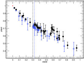
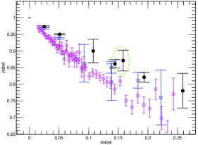
Figure 5: Left: All the numerical results for the pion form factor ($m_{l}=0.02$ circles and $m_{l}=0.01$ squares). Right: Expanded view of low $-q^{2}$-region, now also including experimental results (diamonds) [32, 33] and $f_{\pi\pi}(0)=1$ (star).

The first observation is that our method works very well and that we can indeed compute the pion form factor in the low $|q|^{2}$-regime.

We find that the size of the errors correlates very well with the magnitudes of the momenta of the initial and final state pions. This agrees with the observations of ref. [16] where the statistical noise as a function of the induced meson momentum was investigated numerically in two-point functions and found to increase with the momentum. Similar values of $q^{2}$ may be obtained by pions with very different momenta, and we find that the errors in the form factors are generally smaller if the pions’ momenta are smaller. As an example consider the two results for the pion form factor at the two neighbouring values of $-q^{2}\approx 0.14\,{\rm GeV}^{2}$ and $0.16\,{\rm GeV}^{2}$ for $am_{l}=0.02$ which we indicate by the dashed circle in the right hand plot in fig. 5. In both cases the pion at the sink has a small momentum, $|ap|=0$ and $0.1$, respectively. At the source however the pion’s momentum is $0.25$ in the one case (smaller error bar) and $0.39$ in the other case (larger error bar). In addition, in some cases we achieve a reduction in the error by averaging results for the form factor at degenerate values of the momentum transfer.

3.4 Fits to the Pion Form Factor

Fig. 5 contains the main results of our study for the pion form factor. They are very encouraging, clearly demonstrating the feasibility of the method. Ultimately of course, after performing our large scale simulation, we will wish to compare our results with experimental measurements, but at this stage we can only perform some rudimentary analyses. In particular we investigate various fit-ansätze for our present data with the aim of extracting the pion’s charge radius,

$$\langle r_{\pi}^{2}\rangle=6{df_{\pi\pi}\over dq^{2}}\Big{|}_{q^{2}=0}\,,$$ (23)

which has also been measured in various experiments. For a qualitative comparison of our data to experiment at low values of $|q^{2}|$ we have added the experimental data of refs. [32] and [33] to the r.h.s. plot in fig. 5. We note, that there also exist new measurements of the Pion form factor at larger values of $|q^{2}|$ [34, 35].

One approach is to use a pole-dominance (PD) ansatz of the form:

$$f_{\pi\pi,{\rm PD}}(q^{2})=\frac{n}{1-{q^{2}}/{M^{2}_{\rm PD}(m_{\pi})}}\,,$$ (24)

where the pole mass is related to the pion charge radius by $M_{\rm PD}^{2}=6/\langle r_{\pi}^{2}\rangle_{\rm PD}$. Note that for lattice data $n=1$, whereas for experimental data one either also sets $n=1$ or leaves it as a free parameter due to uncertainties in the overall normalization (see [36] for example). In order to extract the physical value of the charge radius from lattice data one determines $M_{\rm PD}^{2}(m_{\pi})$ for various values of $m_{\pi}$ and extrapolates the pole mass to the chiral limit (cf. e.g. [10]). Since we only have data for two values of the pion mass we will not extrapolate $M_{\rm PD}^{2}(m_{\pi})$ here and merely compare the fit results at fixed pion mass with the ones from the polynomial ansätze,

$$f_{\pi\pi,{\rm lin}}(q^{2})=1+\frac{1}{6}\langle r_{\pi}^{2}\rangle_{\rm lin}\,q^{2}\;\;{\rm and}\;\;f_{\pi\pi,{\rm quad}}(q^{2})=1+\frac{1}{6}\langle r_{\pi}^{2}\rangle_{\rm quad}\,q^{2}+c_{\pi}\,q^{4}\,.$$ (25)

Other ansätze are guided by the prediction of the chiral effective theory [37, 38, 39, 40] where the pion form factor is a well-studied observable [41, 42, 36]. Here we quote the result at next-to-leading order (NLO) [41, 42],

$$f_{\pi\pi,{NLO}}(q^{2})=1+\frac{1}{f_{\pi}^{2}}\left\{2L_{9}^{r}q^{2}+2\tilde{\mathcal{H}}(m_{\pi}^{2},q^{2})+\tilde{\mathcal{H}}(m_{K}^{2},q^{2})\right\}$$ (26)

where $f_{\pi}=92.4(5)(3)$MeV is the physical pion decay constant [43], $L_{9}^{r}$ the only low energy constant relevant at this order of the effective theory and we define

$$\tilde{\mathcal{H}}(m^{2},q^{2}) = q^{2}\left(\frac{5}{576\pi^{2}}-\frac{1}{192\pi^{2}}\log(m^{2}/\mu^{2})\right)-\frac{1}{24\pi^{2}}m^{2}$$ (27)

$$+\left(\frac{1}{96\pi^{2}}\frac{m^{2}}{q^{2}}-\frac{1}{384\pi^{2}}\right)\tilde{\nu}(m^{2},q^{2})\log\left[\frac{2m^{2}-q^{2}-\tilde{\nu}(m^{2},q^{2})}{2m^{2}-q^{2}+\tilde{\nu}(m^{2},q^{2})}\right]\,,$$

with $\tilde{\nu}(m^{2},q^{2})=\sqrt{q^{4}-4q^{2}m^{2}}$.

We have carried out the following fits:

• $\langle r_{\pi}^{2}\rangle$ from fits of (24), (25) and (26) to the lattice data at the unphysical values of the quark mass $am_{l}=0.02$ and $0.01$;

• $\langle r_{\pi}^{2}\rangle_{\chi}$ and $L_{9}^{r}$, where the subscript $\chi$ indicates that the chiral limit has been taken, from global fits to the results at the two pion masses using the NLO expression (26),

• $\langle r_{\pi}^{2}\rangle_{\chi}$ from global fits to the lattice results at the two pion masses using the phenomenologically motivated ansatz

  $$f_{\pi\pi,{\rm pheno}}(q^{2})=f_{\pi\pi,NLO}(q^{2})+c_{1}q^{2}m_{\pi}^{2}+c_{2}q^{2}m_{K}^{2}+c_{3}q^{4}\,.$$ (28)

The results are summarized in fig. 6 and table 2. The plots show how the result of each fit changes under a variation of the range in $q^{2}$ for the various fit functions discussed above. We keep the lowest point in the fit to the $q^{2}$ behaviour fixed at $q^{2}=0$ and vary the upper limit. When we quote the lattice results extrapolated to the chiral limit we mean the point defined by $m_{\pi}=140$ MeV and $m_{K}=494$ MeV. For the final results which we quote in table 2 we chose the upper limit of the fit range to be $\approx 0.1\,{\rm GeV}^{2}$ in the case of the fits A) and B) and about $0.35\,{\rm GeV}^{2}$ for fit C).

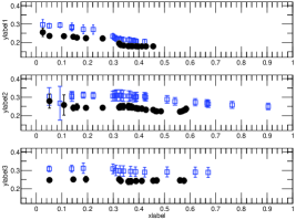
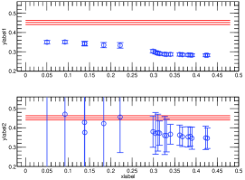
Figure 6: The plots show results from fits to the pion form factor with various fit functions. Left: Results for the charge radius at $am_{l}=0.02$ (black circles) and $am_{l}=0.01$ (blue squares) for linear, quadratic and pole dominance ansatz, respectively. Right: Fits B) and C) compared to the PDG value for the charge radius.

	fit		$\langle r_{\pi}^{2}\rangle|_{0.01}/{\rm fm}^{2}$	$\langle r_{\pi}^{2}\rangle|_{0.02}/{\rm fm}^{2}$
A)	lin.	eq. (25)	0.294(13)	0.234(10)
	quad.	eq. (25)	0.311(16)	0.242(13)
	PD	eq. (24)	0.297(28)	0.239(17)

fit	$\langle r_{\pi}^{2}\rangle_{\chi}/{\rm fm}^{2}$	$L_{9}^{r}(m_{\rho})|_{\chi}$
B)	0.351(8)	0.0050(2)
C)	0.37(5)	0.006(2)

Table 2: Results of pion form factor fits.

All the fits in case A) for the same quark mass are compatible within errors for small values of $|q^{2}|$. The linear fit ansatz starts deviating from the results of the quadratic and PD ansatz between $0.2$ and $0.3\,{\rm GeV}^{2}$. The second order polynomial ansatz and the PD ansatz turn out to be stable and rather constant in the error over a large range of $q^{2}$. We observe a smaller error for the result of the linear fit for small values of the momentum transfer and in this region this is therefore the preferred ansatz.

For case B) we used eq. (26) in a global fit over the results for $am_{l}=0.01$ and $am_{l}=0.02$ and try to obtain a prediction for the charge radius in the chiral limit or equivalently for the low energy constant $L_{9}^{r}$ (we set $\mu=m_{\rho}=0.77$ GeV). For the results which we quote we choose values extracted from the fit including all data points in the interval $q^{2}\in[0,0.1]{\rm GeV^{2}}$. The results are plotted in the upper r.h.s. plot of fig. 6. The blue circles correspond to our lattice results for the charge radius and we indicate the PDG value $\langle r_{\pi}^{2}\rangle=0.452(11){\rm fm}^{2}$ [43] by the horizontal line with error band. Our results disagree very significantly with the PDG value indicating that our quark masses are too heavy to be described by NLO chiral perturbation theory. This conclusion is reinforced by the fact that the values for $L_{9}^{r}$ as determined independently at $am_{l}=0.01$ and $am_{l}=0.02$ are significantly different: $L_{9}^{r}|_{am_{l}=0.01}=0.0056(3)$ and $L_{9}^{r}|_{am_{l}=0.02}=0.0048(2)$. For comparison we also quote the value $L_{9}^{r}=0.00593(43)$ determined by Bijnens [36] using experimental data together with next-to-next-to-leading order chiral perturabation theory.

The results for fit C) are summarized in the lower r.h.s. plot in fig. 6. This global fit of the phenomenologically motivated ansatz (28) leads to results for the charge radius with larger errors. The results which we quote in table 2 correspond to the values extracted from the fit including all data points in the interval $q^{2}\in[0,0.35]{\rm GeV^{2}}$.

4 Conclusions

In this paper we have demonstrated the feasibility of using partially twisted boundary conditions to compute weak and electromagnetic form factors. The technique allows the form factors to be evaluated for any choice of momentum transfer, $q$, within the range of hadronic momenta such that lattice artefacts are small. We have illustrated the techniques for two phenomenologically interesting quantities, the evaluation of the form factors for $K_{\ell 3}$ decays directly at $q^{2}=0$ (thus avoiding the need for an interpolation in $q^{2}$) and of the electromagnetic form factor of the pion at small momentum transfers (thus enabling us to evaluate the pion’s charge radius without extrapolation of the results from large values of $-q^{2}$).

The computations described here were intended to demonstrate the proof of concept, and as such were limited both in statistics and in the lattice parameters. In particular we only compute the form factors for two values of $m_{u,d}$ and hence any investigation of the chiral behaviour is restricted. The next step will be to implement the technique in a large scale simulation which will enable us to overcome the limitations of this feasibility study and to obtain results with the systematic uncertainties under control.

Acknowledgements: We warmly thank Johan Bijnens and Giovanni Villadoro for very helpful discussions.

We gratefully acknowledge the QCDOC design team for developing the QCDOC supercomputer used in these calculations. The development and the computers used in this calculation were funded by the U.S. DOE grant DE-FG02-92ER40699, PPARC JIF grant PPA/J/S/1998/00756 and by RIKEN. We thank the University of Edinburgh, PPARC, RIKEN, BNL and the U.S. DOE for providing these facilities. This work was supported by PPARC grants PPA/G/O/2002/00465, PPA/G/S/2002/00467, PP/D000211/1, PP/D000238/1.

References

- [1] D. Becirevic et al., The vector form factor at zero momentum transfer on the lattice, Nucl. Phys. B705 (2005) 339–362, [hep-ph/0403217].
- [2] D. Becirevic et al., -breaking effects in kaon and hyperon semileptonic decays from lattice QCD, Eur. Phys. J. A24S1 (2005) 69–73, [hep-lat/0411016].
- [3] JLQCD Collaboration, N. Tsutsui et al., Kaon semileptonic decay form factors in two-flavor QCD, PoS LAT2005 (2006) 357, [hep-lat/0510068].
- [4] C. Dawson, T. Izubuchi, T. Kaneko, S. Sasaki, and A. Soni, Vector form factor in semileptonic decay with two flavors of dynamical domain-wall quarks, Phys. Rev. D74 (2006) 114502, [hep-ph/0607162].
- [5] D. J. Antonio et al., form factor with dynamical domain wall fermions, hep-lat/0610080.
- [6] D. J. Antonio et al., form factor with dynamical domain wall fermions: A progress report, hep-lat/0702026.
- [7] D. Guadagnoli, F. Mescia, and S. Simula, Lattice study of semileptonic form factors with twisted boundary conditions, Phys. Rev. D73 (2006) 114504, [hep-lat/0512020].
- [8] Lattice Hadron Physics Collaboration, F. D. R. Bonnet, R. G. Edwards, G. T. Fleming, R. Lewis, and D. G. Richards, Lattice computations of the pion form factor, Phys. Rev. D72 (2005) 054506, [hep-lat/0411028].
- [9] Bern-Graz-Regensburg (BGR) Collaboration, S. Capitani, C. Gattringer, and C. B. Lang, A lattice calculation of the pion form factor with Ginsparg-Wilson-type fermions, Phys. Rev. D73 (2006) 034505, [hep-lat/0511040].
- [10] QCDSF/UKQCD Collaboration, D. Brömmel et al., The pion form factor from lattice QCD with two dynamical flavours, hep-lat/0608021.
- [11] P. F. Bedaque, Aharonov-Bohm effect and nucleon nucleon phase shifts on the lattice, Phys. Lett. B593 (2004) 82–88, [nucl-th/0402051].
- [12] G. M. de Divitiis, R. Petronzio, and N. Tantalo, On the discretization of physical momenta in lattice QCD, Phys. Lett. B595 (2004) 408–413, [hep-lat/0405002].
- [13] C. T. Sachrajda and G. Villadoro, Twisted boundary conditions in lattice simulations, Phys. Lett. B609 (2005) 73–85, [hep-lat/0411033].
- [14] P. F. Bedaque and J.-W. Chen, Twisted valence quarks and hadron interactions on the lattice, Phys. Lett. B616 (2005) 208–214, [hep-lat/0412023].
- [15] B. C. Tiburzi, Twisted quarks and the nucleon axial current, Phys. Lett. B617 (2005) 40–48, [hep-lat/0504002].
- [16] UKQCD Collaboration, J. M. Flynn, A. Jüttner, and C. T. Sachrajda, A numerical study of partially twisted boundary conditions, Phys. Lett. B632 (2006) 313–318, [hep-lat/0506016].
- [17] G. Aarts, C. Allton, J. Foley, S. Hands, and S. Kim, Meson spectral functions at nonzero momentum in hot QCD, hep-lat/0607012.
- [18] B. C. Tiburzi, Flavor twisted boundary conditions and isovector form factors, Phys. Lett. B641 (2006) 342–349, [hep-lat/0607019].
- [19] T. B. Bunton, F. J. Jiang, and B. C. Tiburzi, Extrapolations of lattice meson form factors, Phys. Rev. D74 (2006) 034514, [hep-lat/0607001].
- [20] F. J. Jiang and B. C. Tiburzi, Flavor twisted boundary conditions, pion momentum, and the pion electromagnetic form factor, hep-lat/0610103.
- [21] D. B. Kaplan, A method for simulating chiral fermions on the lattice, Phys. Lett. B288 (1992) 342–347, [hep-lat/9206013].
- [22] Y. Shamir, Chiral fermions from lattice boundaries, Nucl. Phys. B406 (1993) 90–106, [hep-lat/9303005].
- [23] V. Furman and Y. Shamir, Axial symmetries in lattice QCD with Kaplan fermions, Nucl. Phys. B439 (1995) 54–78, [hep-lat/9405004].
- [24] P. A. Boyle et al., Overview of the QCDSP and QCDOC computer, IBM JRD 492 2/3 351–366.
- [25] P. A. Boyle et al., The QCDOC project, Nucl. Phys. Proc. Suppl. 140 (2005) 169–175.
- [26] P. A. Boyle et al., Hardware and software status of QCDOC, Nucl. Phys. Proc. Suppl. 129 (2004) 838–843, [hep-lat/0309096].
- [27] QCDOC Collaboration, P. A. Boyle, C. Jung, and T. Wettig, The QCDOC supercomputer: Hardware, software, and performance, ECONF C0303241 (2003) THIT003, [hep-lat/0306023].
- [28] D. J. Antonio et al., First results from 2+1-flavor domain wall qcd: Mass spectrum, topology change and chiral symmetry with , hep-lat/0612005.
- [29] T. Takaishi, Heavy quark potential and effective actions on blocked configurations, Phys. Rev. D54 (1996) 1050–1053.
- [30] QCD-TARO Collaboration, P. de Forcrand et al., Renormalization group flow of lattice gauge theory: Numerical studies in a two coupling space, Nucl. Phys. B577 (2000) 263–278, [hep-lat/9911033].
- [31] G. Martinelli and C. T. Sachrajda, A lattice study of nucleon structure, Nucl. Phys. B316 (1989) 355.
- [32] NA7 Collaboration, S. R. Amendolia et al., A measurement of the space - like pion electromagnetic form-factor, Nucl. Phys. B277 (1986) 168.
- [33] E. B. Dally et al., Elastic scattering measurement of the negative pion radius, Phys. Rev. Lett. 48 (1982) 375–378.
- [34] Fpi-1 Collaboration, V. Tadevosyan et al., Determination of the pion charge form factor for , nucl-ex/0607007.
- [35] Fpi2 Collaboration, T. Horn et al., Determination of the charged pion form factor at , Phys. Rev. Lett. 97 (2006) 192001, [nucl-ex/0607005].
- [36] J. Bijnens and P. Talavera, Pion and kaon electromagnetic form factors, JHEP 03 (2002) 046, [hep-ph/0203049].
- [37] S. Weinberg, Phenomenological Lagrangians, Physica A96 (1979) 327.
- [38] H. Pagels, Departures from chiral symmetry: A review, Phys. Rept. 16 (1975) 219.
- [39] J. Gasser and H. Leutwyler, Chiral perturbation theory to one loop, Ann. Phys. 158 (1984) 142.
- [40] J. Gasser and H. Leutwyler, Chiral perturbation theory: Expansions in the mass of the strange quark, Nucl. Phys. B250 (1985) 465.
- [41] J. Gasser and H. Leutwyler, Low-energy expansion of meson form-factors, Nucl. Phys. B250 (1985) 517–538.
- [42] J. Bijnens and F. Cornet, Two pion production in photon-photon collisions, Nucl. Phys. B296 (1988) 557.
- [43] Particle Data Group Collaboration, W. M. Yao et al., Review of particle physics, J. Phys. G33 (2006) 1–1232.