The Sign Problem via Imaginary Chemical Potential

Abstract

We calculate an analogue of the average phase factor of the staggered fermion determinant at imaginary chemical potential. Our results from the lattice agree well with the analytical predictions in the microscopic regime for both quenched and phase-quenched QCD. We demonstrate that the average phase factor in the microscopic domain is dominated by the lowest-lying Dirac eigenvalues.

I Introduction

The numerical study of QCD at nonzero chemical potential $\mu$ is hobbled by the complex fermion determinant, which precludes straightforward Monte Carlo calculations based on a real measure. Novel approaches to the problem by means of Taylor expansion Forcrand ; Allton ; Gupta ; Levkova , analytic continuation maria ; owe ; Az , or reweighting Glasgow ; fodor are consistent in measuring the response to small chemical potential around the temperature of chiral restoration, but they disagree at higher values of $\mu$. Moreover, there will be fundamental technical difficulties at larger $\mu$ and larger volumes, and at smaller quark masses and lower temperatures: In all these regimes the fluctuations in the phase of the fermion determinant will become severe GSS ; splitrev . Understanding the behavior of the phase of the determinant is thus of crucial importance for the interpretation of lattice data at nonzero chemical potential (see also Ejiri ).

A common laboratory for studying features of the finite-density theory is entered by making $\mu$ imaginary RW ; AKW . Here the determinant is real and ordinary Monte Carlo methods can be used. On the face of it, it appears that this would be useless for studying the phase of the determinant since the phase is strictly zero for all configurations. It is perhaps startling, then, to note that one can define and compute an analogue of the average phase factor at imaginary $\mu$ exp2ith-long . This offers an approach to studying the strength of the sign problem occurring at real chemical potential by means of simulations at imaginary $\mu$. The advantages of this method are that one does not have to deal with the sign problem in order to measure its strength, and that one does not have to deal with eigenvalues that have spread out into the complex plane.

The phase factor of the fermion determinant at real chemical potential is given by

$$e^{2i\theta} = \frac{\det(D+\mu\gamma_{0}+m)}{\det(D+\mu\gamma_{0}+m)^{*}}$$

$$= \frac{\det(D+\mu\gamma_{0}+m)}{\det(D-\mu\gamma_{0}+m)}.$$

Here we have used the fact that when $\mu$ is real, the complex conjugate determinant is obtained by flipping its sign. The average phase factor at real chemical potential is then

$$\left\langle e^{2i\theta(\mu)}\right\rangle=\left\langle\frac{\det(D+\mu\gamma_{0}+m)}{\det(D-\mu\gamma_{0}+m)}\right\rangle.$$ (2)

As in exp2ith-long we define the average phase factor at imaginary $\mu$ by simply substituting $i\mu$ for $\mu$

$$\left\langle e^{2i\theta(i\mu)}\right\rangle\equiv\left\langle\frac{\det(D+i\mu\gamma_{0}+m)}{\det(D-i\mu\gamma_{0}+m)}\right\rangle,$$ (3)

where the parameter $\mu$ is still real. Both determinants in Eq. (3) are now real. We present in this note a numerical study of the phase factor defined in this manner at imaginary $\mu$. In particular we study the dependence on the chemical potental, the quark mass, and the volume. We work in the microscopic domain of QCD (also called the $\epsilon$-regime) GLeps ; LS , where the quark mass $m$ and the chemical potential are chosen to fulfill

$$|\mu|^{2}F_{\pi}^{2}\ll\frac{1}{\sqrt{V}}\quad\textrm{and}\quad m\Sigma\ll\frac{1}{\sqrt{V}},$$ (4)

while the Euclidean volume $V=L^{3}/T$ (where $T$ is the temperature) is taken large,

$$V\Lambda_{\rm QCD}^{4}\gg 1.$$ (5)

Here $\Sigma=\langle\bar{\psi}\psi\rangle$ is the chiral condensate and $F_{\pi}$ is the pion decay constant. Formulas for the average phase factor have recently been derived in this regime exp2ith-letter ; exp2ith-long .

The values of $\Sigma$ and $F_{\pi}$ on the lattices we use were calculated from a two-point spectral correlation function in Refs. DHSS and DHSST-dyn-dat . Given these values, we can make parameter-free comparisons of the numerical measurements of the average phase factor with the analytical predictions. In all cases we study the agreement is within the statistical errors. This confirmation of the analytic predictions at imaginary $\mu$ gives support to the analytic results derived for real $\mu$ where direct lattice tests are harder to obtain. Our results also show that the average phase factor in the microscopic domain is dominated by the lowest-lying eigenvalues of the Dirac operator.

Below we will recall the theoretical predictions in the microscopic domain and their analytic properties as functions of the chemical potential. Then we will compare these to the lattice data.

II Analytical formulas

Our numerical results are based on data obtained in a quenched ensemble and in an ensemble with dynamical fermions given an imaginary isospin chemical potential. Here we present the microscopic formulas obtained for these two cases.

Below we work with standard unimproved staggered fermions at a coupling where the chiral symmetry breaking pattern is identical to that of the continuum theory in the sector of zero topological charge (see e.g. DHNR ). We therefore present the analytical predictions in the trivial topological sector.

II.1 Quenched theory

The average phase factor at real chemical potential in the quenched theory is given by exp2ith-letter ; exp2ith-long

$$\left\langle e^{2i\theta(\mu)}\right\rangle_{N_{f}=0}=1-4\hat{\mu}^{2}I_{0}(\hat{m})K_{0}(\hat{m})-\frac{e^{-2\hat{\mu}^{2}}}{4\hat{\mu}^{2}}e^{-\frac{\hat{m}^{2}}{8\hat{\mu}^{2}}}\int_{\hat{m}}^{\infty}dx\,xe^{-\frac{x^{2}}{8\hat{\mu}^{2}}}K_{0}\left(\frac{x\hat{m}}{4\hat{\mu}^{2}}\right)\left[I_{0}(x)\hat{m}I_{1}(\hat{m})-xI_{1}(x)I_{0}(\hat{m})\right],$$ (6)

where we have defined microscopic variables via

$$\hat{m}\equiv m\Sigma V\quad\textrm{and}\quad\hat{\mu}\equiv\mu F_{\pi}\sqrt{V}.$$ (7)

The formula (6) cannot be continued to imaginary $\mu$ because of the essential singularity of the last term at $\mu=0$. The non-analyticity has its origin in the inverse determinant of the non-hermitian Dirac operator in Eq. (2)—it is due to the eigenvalues with real part larger than the quark mass SVbos ; exp2ith-long . For purely imaginary $\mu$ the eigenvalues remain on the imaginary axis and are thus always inside the quark mass. The nonanalytic term therefore is not expected to appear at imaginary $\mu$. Indeed, a direct calculation at imaginary $\mu$ gives exp2ith-long

$$\left\langle e^{2i\theta(i\mu)}\right\rangle_{N_{f}=0} = 1+4\hat{\mu}^{2}I_{0}(\hat{m})K_{0}(\hat{m}).$$ (8)

As expected the analytic continuation of this result from imaginary values of the chemical potential back to real values gives just the first two terms in Eq. (6). For real $\mu$ the eigenvalue density outside the quark mass is highly suppressed if $\mu\lesssim m_{\pi}/2$. Consequently the first two terms in (6) are dominant when $\mu\lesssim m_{\pi}/2$ (see Fig. 1). The measurement of the average phase factor at imaginary values of $\mu$ is therefore indicative of the strength of the sign problem for real $\mu\lesssim m_{\pi}/2$.

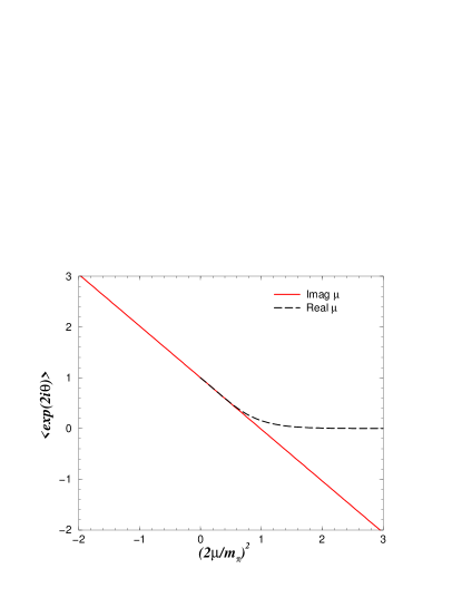
Figure 1: The quenched average phase factor as a function of $(2\mu/m_{\pi})^{2}$ for $\hat{m}=3$. The average phase factor from $\mu^{2}<0$, Eq. (8), gives the solid line when continued via $i\mu\to\mu$. This line agrees with the direct result for real $\mu$, Eq. (6), when $\mu\lesssim m_{\pi}/2$. For larger values of $\mu$ the essential singularity in Eq. (6) at $\mu=0$ becomes important and the analytic continuation fails to reproduce the true result. The same occurs in unquenched QCD.

II.2 Two dynamical flavors with isospin chemical potential

In this theory, also known as the phase-quenched theory, there are two flavors of fermion with opposite values of chemical potential $\pm\mu$. The average phase of the single-flavor determinant is given (for real $\mu$) by

$$\left\langle e^{2i\theta(\mu)}\right\rangle_{1+1^{*}} =$$

$$\frac{\left\langle\frac{\displaystyle\det(D+\mu\gamma_{0}+m)}{\displaystyle\det(D+\mu\gamma_{0}+m)^{*}}\,|\det(D+\mu\gamma_{0}+m)|^{2}\right\rangle}{\langle|\det(D+\mu\gamma_{0}+m)|^{2}\rangle}\,,$$

where the averages on the right-hand side are quenched averages. This simplifies to

$$\left\langle e^{2i\theta(\mu)}\right\rangle_{1+1^{*}} = \frac{\left\langle\det(D+\mu\gamma_{0}+m)^{2}\right\rangle}{\langle|\det(D+\mu\gamma_{0}+m)|^{2}\rangle}=\frac{Z_{N_{f}=2}}{Z_{1+1^{*}}}\,,$$

a ratio of partition functions in ensembles with dynamical fermions. These can be evaluated exactly in the microscopic regime LS ; SplitVerb2 to obtain

$$\left\langle e^{2i\theta(\mu)}\right\rangle_{1+1^{*}}=\frac{I_{0}^{2}(\hat{m})-I_{1}^{2}(\hat{m})}{2\,e^{2\hat{\mu}^{2}}\int_{0}^{1}dt\,te^{-2\hat{\mu}^{2}t^{2}}I_{0}^{2}(\hat{m}t)}$$ (10)

for real $\mu$, with scaling variables as defined in Eq. (7) (note that the numerator, which is $Z_{N_{f}=2}$, does not depend on $\mu$). In this case the average phase factor is analytic at $\mu=0$, because the inverse determinant in the numerator of Eq. (II.2) has been canceled. The average phase factor therefore is

$$\left\langle e^{2i\theta(i\mu)}\right\rangle_{1+1^{*}}=\frac{I_{0}^{2}(\hat{m})-I_{1}^{2}(\hat{m})}{2\,e^{-2\hat{\mu}^{2}}\int_{0}^{1}dt\,te^{2\hat{\mu}^{2}t^{2}}I_{0}^{2}(\hat{m}t)}$$ (11)

for imaginary chemical potential $i\mu$.

III Numerical data

In the lattice theory, we work with standard, unimproved staggered fermions and introduce the chemical potential using the Hasenfratz–Karsch prescription HK . As in the continuum, each operator $D\pm i\mu\gamma_{0}$ is anti-hermitian, and anticommutes with $\gamma_{5}$. Each operator’s eigenvalues therefore come in pairs of opposite sign on the imaginary axis. For each gauge field configuration we measure the two sets of eigenvalues defined by

$$[D(A)+i\mu\gamma_{0}]\psi_{+}^{(j)}=i\lambda_{+}^{(j)}\psi_{+}^{(j)},$$ (12)

$$[D(A)-i\mu\gamma_{0}]\psi_{-}^{(j)}=i\lambda_{-}^{(j)}\psi_{-}^{(j)}.$$ (13)

Thus $\det(D\pm i\mu\gamma_{0}+m)=\prod_{j}(i\lambda_{\pm}^{(j)}+m)$. Combining positive with negative $\lambda$’s, the average phase factor is given by

$$\left\langle e^{2i\theta(i\mu)}\right\rangle = \left\langle\prod_{j=1}^{\infty}\frac{\lambda_{+}^{(j)\,2}+m^{2}}{\lambda_{-}^{(j)\,2}+m^{2}}\right\rangle\equiv\langle\Phi_{+-}\rangle$$ (14)

$$= \left\langle\prod_{j=1}^{\infty}\frac{\lambda_{-}^{(j)\,2}+m^{2}}{\lambda_{+}^{(j)\,2}+m^{2}}\right\rangle\equiv\langle\Phi_{-+}\rangle$$ (15)

where the products run over positive $\lambda$’s only. The equality of $\langle\Phi_{+-}\rangle$ and $\langle\Phi_{-+}\rangle$ follows from charge conjugation symmetry, which exchanges $\lambda_{+}$ with $\lambda_{-}$ and is true in both the quenched and the phase-quenched theory (but not in the unquenched theory). With finite statistics, the two estimators $\Phi_{+-}$ and $\Phi_{-+}$ give distinct measurements of the average phase.

III.1 Quenched theory

Our quenched eigenvalue data are a combination of data used in Ref. DHSS with new data. We simulated the SU(3) gauge theory with the plaquette action at $\beta=5.7$ on lattices with $8^{4}$ and $12^{4}$ sites. For each gauge configuration we calculated the smallest 24 pairs of positive eigenvalues $\lambda_{\pm}^{(j)}$.

On the smaller lattice, we chose two values of the chemical potential: $a\mu=0.01$ and $a\mu=0.1$. In Ref. DHSS we determined $F_{\pi}$ and $\Sigma$, giving the scaled values $\hat{\mu}=0.159$ and $\hat{\mu}=1.59$, respectively; also $\Sigma V/a=1039$, which permits converting the lattice masses $am$ into scaled masses $\hat{m}$. With these values we can make a parameter-free comparison between the analytical prediction (8) and the measurement of the (truncated) average phase factor. The result for $a\mu=0.01$, based on data from Ref. DHSS , is shown in Fig. 2. The agreement is well within the statistical error bars.

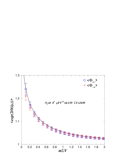
Figure 2: The average phase factor calculated via Eq. (14) (circles) and via Eq. (15) (crosses) from the lowest 24 positive eigenvalues of the staggered Dirac operator on an $8^{4}$ lattice, for fixed chemical potential $a\mu=0.01$ as a function of the scaled quark mass; 4000 configurations. The full line is the analytical microscopic prediction using the parameters determined in Ref. DHSS .

The value $a\mu=0.01$ was chosen in Ref. DHSS to ensure that the scaling variable $\hat{\mu}$ was roughly 1/10, since this facilitates the determination of $F_{\pi}$. At such small values of $\mu$ the shift of the eigenvalues due to the imaginary chemical potential is small compared to the average level spacing. This was our motivation in running a new quenched simulation in order to calculate eigenvalues with the larger value $a\mu=0.1$. The result is shown in Fig. 3; again the agreement with Eq. (8) is good. Note that in this case $\mu L=0.8$ which is pushing the limit of the microscopic domain.

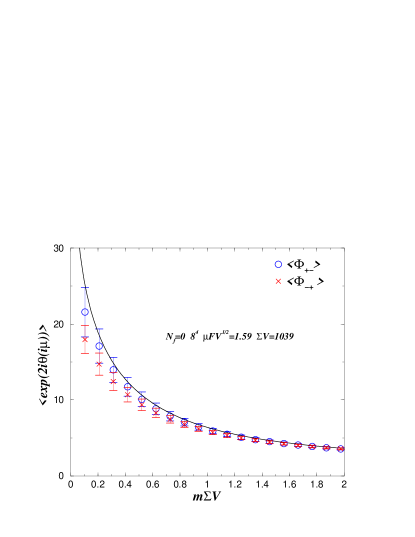
Figure 3: As in Fig. 2 but with $a\mu=0.1$; 6068 configurations.

Since $m$ is not a dynamical parameter of the quenched simulation, the data points for different values of $m$ are highly correlated, and the variation among them is systematic, not statistical. In effect, $m$ determines which eigenvalues contribute the most to the average phase in Eqs. (14) and (15). When $m$ is small, all eigenvalues contribute to the phase; the smallest eigenvalues cause large fluctuations, while the large eigenvalues show but little dependence on $\mu$ and thus contribute little to the ratio. When $m$ is large it eliminates the effect of small eigenvalues on the phase. Therefore as $m$ approaches the largest of the calculated eigenvalues there is a systematic deviation from the analytic curve. We illustrate this by cutting the number of calculated eigenvalues to 10. Figure 4 shows the deviation from the analytic curve as $m\Sigma V$ approaches $\lambda^{(10)}\Sigma V\sim 30$.

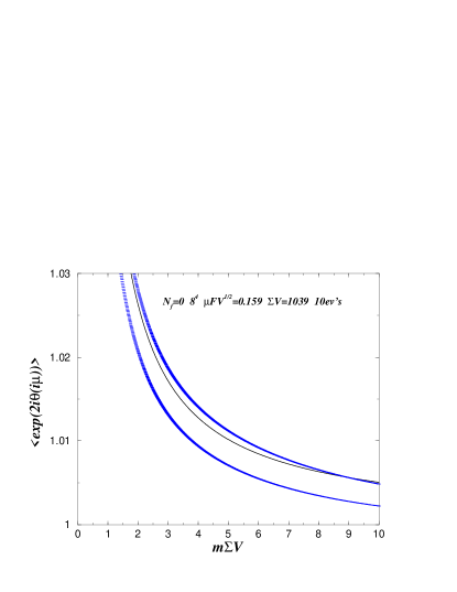
Figure 4: Same eigenvalue data as in Fig. 2, but retaining only 10 eigenvalues. As the quark mass approaches the largest retained eigenvalue ($\lambda^{(10)}\Sigma V\sim 30$) we observe that the error band drops below the analytic curve (thin line).

For the larger lattice, with $12^{4}$ sites, we use data from Ref. DHSS with $a\mu=0.002$. In Ref. DHSS we determined that $\hat{\mu}=\mu F_{\pi}\sqrt{V}=0.159$ and $\Sigma V/a=5259$. Again we can compare the analytical prediction (8) to the measurement of the truncated average phase factor without free parameters, as shown in Fig. 5. The agreement is clear, although statistically weaker than for the smaller lattice.

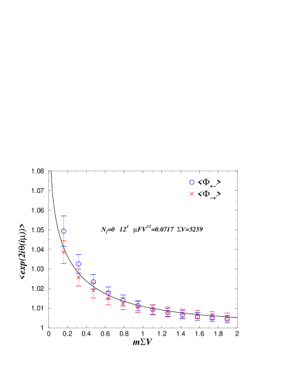
Figure 5: As in Fig. 2, but for the $12^{4}$ lattice; 2000 configurations.

III.2 Two dynamical flavors

For the two-flavor theory with imaginary isospin chemical potential we use eigenvalue data calculated in the long runs of Ref. DHSST-dyn-dat , which should be consulted for numerical details. The lattice theory is based on the plaquette action and unimproved staggered fermions, simulated at $\beta=4.2$ with volume $6^{4}$. We have data for two masses, $am=0.002$ and 0.005, and the imaginary chemical potential coupled to isospin is $a\mu=0.0055$. A determination DHSST-dyn-dat of $aF_{\pi}$ gives $\hat{\mu}=0.1338$.

For the smaller quark mass, $am=0.002$, we calculated DHSST-dyn-dat that $\hat{m}=m\Sigma V=3.318$. From the lowest 24 eigenvalues we measure

$$\left\langle\Phi_{+-}\right\rangle_{1+1^{*}} = 1.0092\pm 0.0020$$ (16)

$$\left\langle\Phi_{-+}\right\rangle_{1+1^{*}} = 1.0082\pm 0.0020.$$ (17)

The analytical prediction for the average phase factor (11) is

$$\left\langle e^{2i\theta(i\mu)}\right\rangle_{1+1^{*}}=1.0094,$$ (18)

in agreement with the numerical averages.

For the larger quark mass ($ma=0.005$) we have $m\Sigma V=8.295$. From the lowest 24 eigenvalues we compute

$$\left\langle\Phi_{+-}\right\rangle_{1+1^{*}} = 1.0036\pm 0.0030$$ (19)

$$\left\langle\Phi_{-+}\right\rangle_{1+1^{*}} = 1.0032\pm 0.0030.$$ (20)

The analytical formula (11) gives

$$\left\langle e^{2i\theta(i\mu)}\right\rangle_{1+1^{*}}=1.0041.$$ (21)

Here also we see satisfactory agreement with theory, although the deviation from unity is not really significant.

IV Conclusions

We have computed an analogue of the complex phase factor of the fermion determinant at imaginary values of the chemical potential. The results have been used as a parameter-free test of the predictions from the microscopic domain of QCD. In the quenched as well as in the dynamical cases studied the numerical and analytical results are in agreement. Furthermore, we have demonstrated that the phase factor in the microscopic domain is dominated by the low-lying Dirac eigenvalues.

We hope that this first numerical study of the phase factor at imaginary chemical potential will encourage studies also outside the microscopic domain.

- (1) S. Choe et al., Phys. Rev. D 65, 054501 (2002); I. Pushkina et al. [QCD-TARO Collaboration], Phys. Lett. B 609, 265 (2005) [hep-lat/0410017].
- (2) C. R. Allton et al., Phys. Rev. D 66, 074507 (2002) [hep-lat/0204010]; ibid. 68, 014507 (2003) [hep-lat/0305007]; ibid. 71, 054508 (2005) [hep-lat/0501030].
- (3) R. V. Gavai and S. Gupta, Phys. Rev. D 68, 034506 (2003) [hep-lat/0303013]; ibid. 71, 114014 (2005) [hep-lat/0412035];
- (4) C. Bernard et al., PoS LAT2006, 139 (2006) [hep-lat/0610017].
- (5) M. D’Elia and M. P. Lombardo, Phys. Rev. D 67, 014505 (2003) [hep-lat/0209146]; ibid. 70, 074509 (2004) [hep-lat/0406012];
- (6) P. de Forcrand and O. Philipsen, Nucl. Phys. B 642, 290 (2002) [hep-lat/0205016]; ibid. 673, 170 (2003) [hep-lat/0307020]; J. High Energy Phys. 0701, 077 (2007) [hep-lat/0607017].
- (7) V. Azcoiti, G. Di Carlo, A. Galante and V. Laliena, J. High Energy Phys. 0412, 010 (2004) [hep-lat/0409157]; Nucl. Phys. B 723, 77 (2005) [hep-lat/0503010].
- (8) I. M. Barbour et al., Phys. Rev. D 56, 7063 (1997) [hep-lat/9705038] and references therein.
- (9) Z. Fodor and S. D. Katz, Phys. Lett. B 534, 87 (2002) [hep-lat/0104001]; J. High Energy Phys. 0203, 014 (2002) [hep-lat/0106002]; ibid. 0404, 050 (2004) [hep-lat/0402006]; Z. Fodor, S. D. Katz and C. Schmidt, arXiv:hep-lat/0701022.
- (10) M. Golterman, Y. Shamir and B. Svetitsky, Phys. Rev. D 74, 071501 (2006) [hep-lat/0602026]; B. Svetitsky, Y. Shamir and M. Golterman, PoS LAT2006, 148 (2006) [hep-lat/0609051].
- (11) K. Splittorff, PoS LAT2006 023 (2006) [hep-lat/0610072].
- (12) S. Ejiri, Phys. Rev. D 69, 094506 (2004) [hep-lat/0401012]; ibid. 73, 054502 (2006) [hep-lat/0506023].
- (13) A. Roberge and N. Weiss, Nucl. Phys. B 275, 734 (1986).
- (14) M. Alford, A. Kapustin, and F. Wilczek, Phys. Rev. D 59 (1999) 054502.
- (15) K. Splittorff and J. J. M. Verbaarschot, hep-lat/0702011.
- (16) J. Gasser and H. Leutwyler, Phys. Lett. B 188, 477 (1987).
- (17) H. Leutwyler and A. Smilga, Phys. Rev. D 46, 5607 (1992).
- (18) K. Splittorff and J. J. M. Verbaarschot, Phys. Rev. Lett. 98, 031601 (2007) [hep-lat/0609076].
- (19) P. H. Damgaard, U. M. Heller, K. Splittorff and B. Svetitsky, Phys. Rev. D 72, 091501 (2005) [hep-lat/0508029].
- (20) P. H. Damgaard, U. M. Heller, K. Splittorff, B. Svetitsky and D. Toublan, Phys. Rev. D 73, 074023 (2006) [hep-lat/0602030].
- (21) P. H. Damgaard, U. M. Heller, R. Niclasen and K. Rummukainen, Phys. Rev. D 61, 014501 (2000) [hep-lat/9907019].
- (22) K. Splittorff and J. J. M. Verbaarschot, Nucl. Phys. B 757, 259 (2006) [hep-th/0605143].
- (23) K. Splittorff and J. J. M. Verbaarschot, Nucl. Phys. B 683, 467 (2004) [hep-th/0310271].
- (24) P. Hasenfratz and F. Karsch, Phys. Lett. B 125, 308 (1983).
- (25) J. C. Osborn, Phys. Rev. Lett. 93, 222001 (2004) [hep-th/0403131].
- (26) G. Akemann, J. C. Osborn, K. Splittorff and J. J. M. Verbaarschot, Nucl. Phys. B 712, 287 (2005) [hep-th/0411030].