Abelian dominance in local unitary gauges and without gauge-fixing in pure SU(2) QCD

Abstract:

We perform lattice Monte-Carlo simulations of pure $SU(2)$ QCD using the multi-level method. We find Abelian dominance in local unitary gauges such as those diagonalizing a plaquette. A static potential described by Abelian link fields alone gives us the same string tension as that of a non-Abelian potential. Abelian dominance of the string tension and Abelian flux tube profiles are observed also without gauge-fixing, i.e., without any Abelian projection. On the basis of these results, we propose a simple gauge-independent Abelian confinement scenario without any Abelian projection. All color components of the non-Abelian field strength become Abelian dominant in the infrared region. The Abelian dual Meissner effect works in any color direction. Abelian neutral states in any color directions which are just non-Abelian color-singlet can exist as a physical state. In this way, the non-Abelian color confinement could be understood in the framework of the Abelian dual Meissner effect.

1 Abelian dominance in Abelian projection.

The Abelian dual Meissner effect is believed to be the color confinement mechanism in QCD [1][2]. In this model Abelian gauge fields and Abelian monopoles play very important roles. How to extract Abelian monopoles from non-Abelian QCD is a problem. In 1981 ’tHooft suggested an Abelian projection method in which the Abelian degrees of freedom can be extracted [3]. A partial gauge-fixing is performed in the Abelian projection. Only $U^{N_{c}-1}(1)$ subgroup remains unbroken after the Abelian projection. On lattice, the Abelian gauge fields $\theta_{n,\mu}$ are defined by the following way: (Here we consider the SU(2) case for simplicity.)

$$U_{n,\mu}^{G}=C_{n,\mu}u_{n,\mu},$$ (1)

$$u_{n,\mu}=\mbox{diag}(e^{\theta_{n,\mu}},e^{-\theta_{n,\mu}}),$$ (2)

where $U_{n,\mu}^{G}$ is a non-Abelian link fields after the partial gauge-fixing using a gauge transformation matrix G. $C_{n,\mu}$ is an off-diagonal field. The maximally Abelian(MA) gauge ,where link variables are abelianized as much as possible, is the most famous gauge-fixing condition in the Abelian projection. Numerically the string tension calculated from Abelian parts reproduces well the original one in MA gauge[4][5]. It is called as Abelian dominance. There are many results which suggest the Abelian scenario in MA gauge(e.g. flux tube profiles[6]). In MA gauge, the Abelian scenario based on the Abelian dual Meissner effect works good. However there is a serious problem in the Abelian scenario. Namely good results suggesting the success of the Abelian scenario are obtained with only a few non-local gauges which are similar to MA gauge. Particularly the Abelian scenario has not been observed in local unitary gauges such as F12 gauge [4][7][8]. We call it ’gauge dependence problem of the Abelian scenario’. In this short note, we investigate this problem with the method of high precision simulations.

2 Abelian dominance in local unitary gauges.

In local gauges, we know quantum fluctuations are very large and there are huge noise. On the other hand, in non-local gauges like MA gauge, vacuum fluctuations are small and we have been able to observe physical quantities very clearly. There are much difference of quantum fluctuations between MA gauge and local unitary gauges. Hence to extract physical signals in local unitary gauges, high precision investigations are necessary. But such a study has not been done so far. We perform such high precision investigations in local unitary gauges using the multi-level method developed by Lűscher and Weisz[9].

2.1 The multi-level method

The multi-level method is a powerful noise reduction method[9]. This method is effective only with respect to local operators. For example it is very useful to measure Polyakov loop correlation functions. The procedure is the following: 1. Lattice is divided into $N_{s}$ sublattices. 2. A sublattice average of operators is taken. 3. The link variables are replaced using gauge update except for the spatial links at the boundary of the sublattice. (it is called internal update.) 4. Step 2, 3 are repeated until stable values for the sublattice average of operators are obtained. Now we adopt this method in the Abelian projection using local unitary gauges. Then gauge-fixing and the Abelian projection steps are implemented in each internal update. And operators are constructed by Abelian link fields. As a gauge-fixing condition, we consider local unitary gauges consistent with the multi-level method.

2.2 Local unitary gauge.

We consider three local unitary gauges here. The first one is a F12 gauge which makes 1-2 plane plaquette diagonal.

$$G_{F12,n}\left(U_{n,1}U_{n+\hat{1},2}U_{n+\hat{2},1}^{\dagger}U_{n,2}^{\dagger}\right)G_{F12,n}^{\dagger}=\mbox{(diagonal)}.$$ (3)

The second is a F123 gauge similar to the F12 gauge. Its gauge-fixing matrix makes a 1-2-3 cube-like operator in Fig.1 diagonal.

$$G_{F123,n}\left(U_{n,1}U_{n+\hat{1},2}U_{n+\hat{1}+\hat{2},3}U_{n+\hat{2}+\hat{3},1}^{\dagger}U_{n+\hat{3},2}^{\dagger}U_{n,3}^{\dagger}\right)G_{F123,n}^{\dagger}=\mbox{(diagonal)}.$$ (4)

The third is a spatial Polyakov line (SPL) gauge similar to Polyakov gauge. The gauge-fixing matrix makes spatial Polyakov line operators in Fig.1 diagonal.

$$G_{SPL,n}\left(\sum_{\mu=1}^{3}\prod_{i=1}^{N_{s}}U_{n+(i-1)\hat{\mu},\mu}\right)G_{SPL,n}^{\dagger}=\mbox{(diagonal)}.$$ (5)

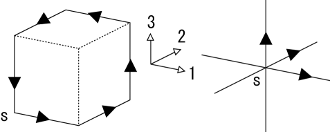
Figure 1: The left figure shows the cube operator diagonalized in the F123 gauge. The right is the set of spatial Polyakov lines used in the SPL gauge.

2.3 Numerical results

We use a simple SU(2) Wilson gauge action. We adopt the coupling constant $\beta=2.5$ which corresponds to the lattice spacing $a(\beta=2.5)=0.082(2)[fm]$. The lattice size is $24^{4}$. For the multi-level method, the number of sublattices is 6, the sublattice size is 4 and iterations of internal updates are over 80000.

First we show an Abelian static potential in F12 gauge and compare it with non-Abelian one. In the figure 2(left) Abelian dominance is seen clearly. This is a very interesting result. Note that the Coulomb part is different from that in the non-Abelian potential. The Coulomb part is also different in MA gauge. Next we show in 2(right) Abelian potentials in other two local unitary gauges. The F123 gauge gives us almost similar results as in F12 gauge. On the other hand, the SPL gauge gives bigger Coulomb coefficient. Nevertheless, explicit values of the fitted string tension shown in Table 1 are the same within the statistical errors. We could conclude that Abelian dominance is confirmed also in these local unitary gauges.

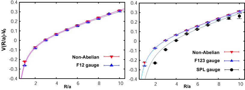
Figure 2: Left is a static potential in F12 gauge in comparison with the non-Abelian potential. Right is a potential in F123 gauge and SPL gauge in comparison with the non-Abelian potential. The solid lines show a fitted function ($\sigma R-{c/R}+V_{0}$).

Table 1: Fitted string tensions($\beta=2.5$). The region for fitting is $R/a=2\sim 10$.

	NonAbelian	F12 gauge	F123 gauge	SPL
String tension $\sigma$	0.034(2)	0.034(2)	0.034(2)	0.034(2)
Coulomb coefficient $c$	0.29(1)	0.29(1)	0.28(1)	0.65(3)

3 Abelian dominance without gauge-fixing.

The Abelian dominance is found to be seen in local unitary gauges where quantum fluctuations are large. This suggests that Abelian dominance works in any Abelian projection scheme, although it is impossible to investigate all gauge-fixing conditions. If it is true, gauge-fixing may not be essential in Abelian confinement scenario. To confirm this suggestion, we measure an Abelian static potential and Abelian flux tube profiles without gauge-fixing. In figure 3 we show the Abelian potential without gauge-fixing using the multi-level method. The parameters for the multi-level method are the same as those used in local unitary gauge cases. In no gauge-fixing case Abelian and non-Abelian potentials are quite similar in all regions. This results had been expected analytically by Ogilvie[10]. The fitted string tension $\sigma$ is 0.034(2). This result shows Abelian dominance can be seen without any gauge-fixing.

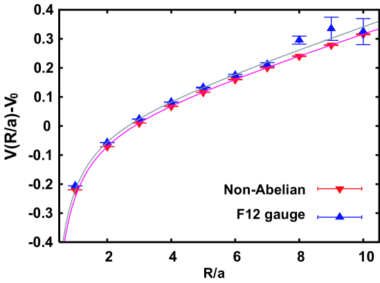
Figure 3: Abelian potential without gauge-fixing in comparison with the non-Abelian potential. The solid lines mean a fitted function ($\sigma R-{c/R}+V_{0}$).

3.1 Abelian flux tube profiles

Abelian flux tube profiles are important observables in understanding the Abelian scenario. For this purpose we calculate correlations between the Wilson loop and Abelian field strength without gauge-fixing. However simple correlation functions between disconnected operators can not observe the profiles, since the Abelian plaquette operator is gauge-variant. Here we measure connected correlation functions to measure the Abelian flux tube profiles without gauge-fixing. Similar investigations were done to measure non-Abelian electric fields around a pair of static quarks by Cea et al. [11] and DiGiacomo et al.[12]. The connected correlation function is defined as follows:

$$\langle{\cal O}_{A}(r)\rangle_{W} = {\langle{1\over 3}\sum_{a}\mbox{Tr}\left[LW(r=0,R,T)L^{\dagger}\sigma^{a}{\cal O}_{A}^{a}(r)\right]\rangle\over\langle\mbox{Tr}\left[W(R,T)\right]\rangle}$$ (6)

where ${\cal O}_{A}$ is an Abelian field strength operator constructed by Abelian link fields, $L$ is a non-Abelian link field connecting the Wilson loop with the Abelian operator and $W$ is the Wilson loop (See figure 4). To avoid the artificial effects of the bridge part $L$ and $L^{\dagger}$, we consider several types of L and then take an average of the results of all types adopted.

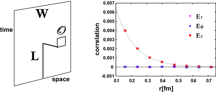
Figure 4: The left shows a connected Wilson loop correlation function. The right figure shows all components of the Abelian electric field. These profiles are studied on a perpendicular plane at the midpoint between the two quarks. The Wilson loops size is ($R\times T$)=($5\times 5$).

In this calculation we use the Iwasaki gauge action[13] . We adopt the coupling constant $\beta=1.20$ which corresponds to the lattice distance $a(\beta=1.20)=0.0792(2)[fm]$. The lattice size is $32^{4}$. After 5000 thermalizations, we have taken 4000 thermalized configurations per 200 sweeps for measurements. To get a good signal-to-noise ratio, the APE smearing technique is used for evaluating Wilson loops[14].

We measured all components of the Abelian electric fields $E_{Ai}$.

$$E_{Ai} = \Theta_{n,4,i}$$ (7)

$$\Theta_{n,\mu,\nu} = \theta_{n,\mu}+\theta_{n+\hat{\mu},\nu}-\theta_{n+\hat{\nu},\mu}-\theta_{n,\nu}$$ (8)

In figure 4 we show that the Abelian electric fields are squeezed. We try to fit using the following function:

$$f(x) = c_{1}\exp(-r/\lambda)+c_{0}.$$ (9)

Here $\lambda$ is the penetration length which is an important quantity in the Abelian dual Meissner effect. The fitted penetration length $\lambda$ is 0.12(2)[fm]. This result is consistent with that in MA gauge in Ref [15]. We find also that all components of the magnetic fields have no correlation with the Wilson loop. These results are consistent with the Abelian scenario.

4 Conjecture and conclusions

We have studied the gauge dependence problem with respect to Abelian confinement scenario. First we have studied extensively Abelian projections in local unitary gauges with the help of the multi-level noise reduction method.

• In local unitary gauges (F12, F123, SPL) Abelian dominance with respect to the string tension is observed very beautifully. The difference is seen only in the Coulomb region.

Next we have investigated if the Abelian confinement scenario can be seen without any gauge-fixing.

• Abelian dominance of the string tension is observed in all regions without any gauge-fixing.

• Abelian electric fields are squeezed and the penetration length observed is consistent with that in MA gauge. Here we have used many vacuum configurations using the Iwasaki improved gauge action on $32^{4}$ lattice.

These results suggest that Abelian confinement scenario works without resort to Abelian projection.

On the basis of the above results, we propose a conjecture of a gauge-independent Abelian confinement scenario;
Each Abelian component in any color direction becomes dominant in the infrared region. Abelian dominance and the Abelian dual Meissner effect are seen in any color direction. A state which is Abelian neutral in any color direction can be a physical state. It is just a color-singlet state. In this way, color confinement can be understood in the framework of Abelian scenario in a gauge-invariant way.
It is very interesting to confirm this conjecture numerically. The investigation is in progress.

Acknowledgments

The authors would like to thank Y. Koma for his simulation code of the multi-level method. The numerical simulations of this work were done using NEC SX7 in RIKEN and NEC SX5 in RCNP. The authors would like to thank RIKEN and RCNP for their support of computer facilities.

References

- [1] S. Mandelstam. Phys. Rept. 23:245–249, 1976.
- [2] Gerard ’t Hooft. Nucl. Phys. B79:276–284, 1974.
- [3] G. ’t Hooft. Nucl. Phys. B190:455, 1981.
- [4] Suzuki, Tsuneo and Yotsuyanagi, Ichiro. Phys. Rev. D42:4257-4260, 1990.
- [5] Bali, Gunnar S. hep-ph/9809351, Talk presented at Quark confinement and the hadron spectrum III(1998)
- [6] Koma, Y. and Koma, M. and Ilgenfritz, Ernst-Michael and Suzuki, T. and Polikarpov, M. I. Phys. Rev. D68:094018, 2003.
- [7] Bernstein, Kenneth and Di Cecio, Giuseppe and Haymaker, Richard W. Phys. Rev. D55:6730-6742, 1997.
- [8] Ito, Shoichi and Park, Tae Woong and Suzuki, Tsuneo and Kitahara, Shun-ichi. Phys. Rev. D67:074504, 2003.
- [9] Luscher, Martin and Weisz, Peter. JHEP 09:010, 2001. JHEP 07:049, 2002.
- [10] Ogilvie, Michael C. Phys. Rev. D59:074505, 1999.
- [11] Cea, Paolo and Cosmai, Leonardo. Phys. Rev. D52:5152-5164, 1995.
- [12] Di Giacomo, Adriano and Maggiore, Michele and Olejnik,Stefan. Phys. Lett. B236:199, 1990. Nucl. Phys. B347:441-460, 1990.
- [13] Y. Iwasaki, Nucl. Phys. B258, 141 (1985). 1983.
- [14] APE, M. Albanese et al., Phys. Lett. B192, 163 (1987).
- [15] Chernodub, M. N. et al., Phys. Rev. D72, 074505 (2005).