Abelian dominance and the dual Meissner effect in local unitary gauges
in SU(2) gluodynamics

Abstract

Performing highly precise Monte-Carlo simulations of SU(2) gluodynamics, we observe for the first time Abelian dominance in the confining part of the static potential in local unitary gauges such as the F12 gauge. We also study the flux-tube profile between the quark and antiquark in these local unitary gauges and find a clear signal of the dual Meissner effect. The Abelian electric field is found to be squeezed into a flux tube by the monopole supercurrent. This feature is the same as that observed in the non-local maximally Abelian gauge. These results suggest that the Abelian confinement scenario is gauge independent. Observing the important role of space-like monopoles in the Polyakov gauge also indicates that the monopoles defined on the lattice do not necessarily correspond to those proposed by ’t Hooft in the context of Abelian projection.

Quark confinement phenomenon remains an important unsolved problem in quantum chromodynamics (QCD) CMI:2000mp . One of the most intriguing conjecture for its mechanism is that the QCD vacuum behaves as a dual superconductor due to magnetic monopole condensation tHooft:1975pu ; Mandelstam:1974pi , i.e., the color flux between a quark and an antiquark is squeezed into a stringlike tube as the Abrikosov vortex Abrikosov:1956sx ; Nielsen:1973cs through the dual Meissner effect, which yields a linear-confining potential. Although it is not straightforward to identify the corresponding monopoles in QCD in contrast to SUSY QCD Seiberg:1994rs or the Georgi-Glashow model 'tHooft:1974qc ; Polyakov:1976fu with scalar fields, it is possible to reduce SU(3) QCD into an Abelian [U(1)]² theory with magnetic monopoles by a partial gauge fixing, also referred to as the Abelian projection tHooft:1981ht , and to accommodate the above dual superconductor scenario Ezawa:1982bf .

However, there are infinite ways of the partial gauge-fixing. Numerically, an Abelian projection with non-local gauges such as the maximally Abelian (MA) gauge Suzuki:1983cg ; Kronfeld:1987ri ; Kronfeld:1987vd has been found to support the Abelian confinement scenario beautifully  Suzuki:1992rw ; Chernodub:1997ay ; Suzuki:1998hc ; Singh:1993jj . On the other hand, the Abelian confinement mechanism has not been observed clearly so far for years in other general gauges in particular, in local unitary gauges Suzuki:1989gp ; Bernstein:1996vr ; Ito:2002zv . This is very unsatisfactory, since the quark confinement mechanism should not depend on a special gauge choice Carmona:2001ja .

It is the purpose of this letter to show for the first time that the Abelian confinement mechanism is observed numerically also in local unitary gauges with the method of highly precise numerical simulations. For numerical simplicity we adopt SU(2) group instead of SU(3), but the essential feature of non-Abelian gauge theory should be the same. As local unitary gauges, we adopt simplest candidates, namely the F12, the F123 and the spatial Polyakov loop (SPL) gauges as well as the original Polyakov (PL) gauge. Applying the multi-level noise reduction method invented by Lüscher and Weisz Luscher:2001up , we investigate the Abelian static potential with high accuracy and find a clear signal of Abelian dominance in its confining part in all local unitary gauges considered. Note that F12 (F123) gauge and PL (SPL) gauge are most typical but are of completely different types. Since we obtain the same results in these different unitary gauges, we expect that the same can be seen also in other local unitary gauges. In addition, we study the flux-tube profile between the quark and antiquark with the vacuum ensemble composed of as many as 4000 thermalized configurations generated by means of the improved Iwasaki action Iwasaki:1985we and observe the squeezing of Abelian electric field into a flux tube due to the magnetic monopole current. This is the dual Meissner effect and the feature is quite similar to that already observed in the MA gauge. The authors expect that the results obtained here are very interesting to general readers, since they strongly suggest that the Abelian dual Meissner effect caused by Abelian monopoles is gauge independent and a correct confinement mechanism.

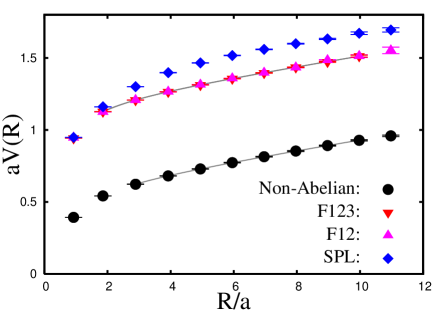
Figure 1: Abelian static potentials in the F123, the F12 and the SPL gauges in comparison with the non-Abelian potential. The solid lines denote the best fitting curves to the function $V_{\rm fit}(R)$.

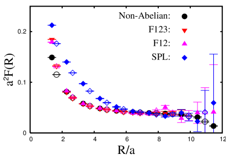
Figure 2: The force in the F123, the F12 and the SPL gauges in comparison with the non-Abelian one. The filled (open) symbols are forces which are defined by using the backward (mid-point) difference.

We generate thermalized gluon configurations using the standard SU(2) Wilson gauge action at the coupling constant $\beta=2.5$ on the lattice $N^{4}=24^{4}$, where the lattice spacing is $a(\beta)=0.0836(8)$ fm. The scale is set from the string tension $\sqrt{\sigma}=440$ MeV. Periodic boundary conditions are imposed in all directions. Then we perform a partial gauge fixing diagonalizing a plaquette operator $X(s)\equiv U_{12}(s)$ [F12 gauge], or an operator $X(s)\equiv U_{1}(s)U_{2}(s+\hat{1})U_{3}(s+\hat{1}+\hat{2})U^{{\dagger}}_{1}(s+\hat{3}+\hat{2})U^{{\dagger}}_{2}(s+\hat{3})U^{{\dagger}}_{3}(s)$ [F123 gauge], or a space-like Polyakov loop $X(s)\equiv\mathcal{P}_{\rm SU(2)}\sum_{k=1}^{3}\prod_{i=0}^{N-1}U_{k}(s+i\hat{k})$ [SPL gauge], or a usual time-like Polyakov loop $X(s)\equiv\prod_{i=0}^{N-1}U_{4}(s+i\hat{4})$ [PL gauge]. After gauge fixing, we decompose SU(2) link variables as

$$U_{\mu}(s)=U^{0}_{\mu}(s)\!+\!i\vec{\sigma}\vec{U}_{\mu}(s)=C_{\mu}(s)\!\left(\begin{array}[]{cc}e^{i\theta_{\mu}(s)}&0\\ 0&e^{-i\theta_{\mu}(s)}\\ \end{array}\right),$$

where $\vec{\sigma}$ is the Pauli matrix, and extract Abelian link variables $\theta_{\mu}(s)=\arctan(U^{3}_{\mu}(s)/U^{0}_{\mu}(s))$ Kronfeld:1987vd . Since the first three gauges contain only space-like link variables, we may apply the multi-level algorithm Luscher:2001up to evaluate the Abelian static potential from the correlator of the Abelian Polyakov loop defined by $P_{A}(\vec{s})=\exp\left[i\sum_{i=0}^{N-1}\theta_{4}(s+i\hat{4})\right]$. For the multi-level method, we choose the temporal extent of a sublattice to be $4a$.

Note that the expectation value of such an U(1) invariant Abelian quantity in some gauges is expressed theoretically by a sum of complicated gauge-invariant quantities composed of operators in various representations Ogilvie:1998wu and hence the numerical results are not predictable.

Table 1: The string tension $\sigma$, the Coulombic coefficient $c$, and the constant $\mu$ obtained by the best fit. FR means the fitting range before tree-level improvement. $\chi^{2}$ is defined by the diagonal components of the covariance matrix and $N_{\rm df}$ is the number of degrees of freedom. $N_{\rm iupd}$ is the number of internal updates used in the multi-level method. $N_{\rm conf}$ is $8$. The errors are estimated by the jackknife method.

	$\sigma a^{2}$	$c$	$\mu a$	FR(R/a)	$\chi^{2}/N_{\rm df}$	$N_{\rm iupd}$
NA	.0348(7)	.243(6)	0.607(4)	3 - 10	0.35	15000
F123	.0350(2)	.239(1)	1.187(1)	2 - 10	0.10	80000
F12	.0345(6)	.244(4)	1.192(3)	2 - 10	1.08	80000

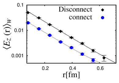
Figure 3: The profile of the Abelian electric field from the connected and disconnected correlators in the MA gauge.

In Fig. 1, we show the Abelian static potential as well as the non-Abelian potential as a function of the $q$-$\bar{q}$ distance $R$, where a tree-level perturbative improvement of the distance is applied to avoid an enhancement of lattice artifacts especially at short distances Necco:2001xg ; Luscher:2002qv . We find that the results in local unitary gauges are remarkably clean. Note that although the number of configurations ($N_{\textrm{conf}}$) for measurements is low, the multi-level algorithm with enough internal updates gives us clear expectation values of the Abelian Polyakov-loop correlators up to as precisely as $10^{-16}$. The slope at large distances looks identical. We may fit the potentials to a usual functional form $V_{\rm fit}(R)=\sigma R-c/R+\mu$ and extract the string tension $\sigma$. The best fitting parameters are summarized in Table 1. In the F12 and the F123 gauges, the string tensions are in almost complete agreement with the non-Abelian one. In the SPL gauge ($N_{\rm conf}=10$ with $N_{\rm iupd}=300000$), however, the Coulombic coefficient becomes so large ($c\approx 0.8$) that we cannot determine the string tension definitely on this small lattice. On the other hand, in all gauges the force, which is defined by differentiating the potential with respect to $R$, shows a good agreement at large distances (see Fig. 2). In the PL gauge, the agreement of Abelian and non-Abelian string tensions is trivial, since non-Abelian Polyakov lines are equal to Abelian ones in this gauge.

Next let us study the dual Meissner effect in local unitary gauges. In this calculation, we employ the improved Iwasaki gauge action with the coupling constant $\beta=1.20$, which corresponds to the lattice spacing $a(\beta)=0.0792(2)$ fm Suzuki:2004dw . The lattice size is $32^{4}$ with periodic boundary conditions. We have taken 4000 thermalized configurations for measurements. To improve a signal-to-noise ratio, the APE smearing technique is applied to the Wilson loop Albanese:1987ds . In addition, although we could measure usual (disconnected) correlators after the gauge-fixing,we evaluate a connected correlator defined by $\langle{\cal O}_{A}(r)\rangle_{W}=\langle\mbox{Tr}\left[LW(R,T)L^{\dagger}\sigma^{3}{\cal O}_{A}^{3}(r)\right]\rangle/\langle\mbox{Tr}\left[W(R,T)\right]\rangle$ for various operators ${\cal O}_{A}$ composed of Abelian link variables in order to get a better signal, where $L$ is a product of non-Abelian link variables called the Schwinger line, connecting the Wilson loop $W$ with the Abelian operator Cea:1995zt ; DiGiacomo:1989yp . $r$ is the minimal distance between $W$ and ${\cal O}_{A}$. As Abelian operators, for instance, we employ the Abelian electric field $E_{i}(s)\equiv\bar{\theta}_{4i}(s)$ and the monopole current $k_{i}(s)\equiv(1/4\pi)\epsilon_{i\nu\rho\sigma}\partial_{\nu}\bar{\theta}_{\rho\sigma}(s+\hat{i})$ where $\theta_{\mu\nu}(s)\equiv\theta_{\mu}(s)+\theta_{\nu}(s+\hat{\mu})-\theta_{\mu}(s+\hat{\nu})-\theta_{\nu}(s)=\bar{\theta}_{\mu\nu}(s)+2\pi n_{\mu\nu}(s)~{}(|\bar{\theta}_{\mu\nu}|<\pi)$ .

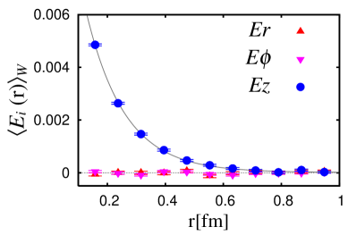
Figure 4: The profile of the Abelian electric field in the F123. The solid line denotes the fitting curve for $\langle E_{z}(r)\rangle_{W}$ to the function $f(r)$.

We first examine the consistency between the result from the usual disconnected correlators Singh:1993jj and the connected one in the MA gauge for $\langle E_{z}(r)\rangle_{W}$. The profile of the electric field is plotted in Fig. 3. We find that while the absolute magnitude of the electric field depends on the type of the correlator, their exponential decay rates look the same. Assuming a functional form $f(r)=c_{1}\exp(-r/\lambda)+c_{0}$, we may estimate the penetration length $\lambda$, which characterizes the strength of the dual Meissner effect. The result is $\lambda=0.133(4)$ fm for the disconnected correlator and $\lambda=0.131(10)$ fm for the connected one in the case of $W(5a,7a)$. $c_{0}$ is consistent with zero in each case. This indicates that the result of the connected correlator can be consistent with that of disconnected one.

In Fig. 4, we show the Abelian electric field profile in the F123 gauge for $W(5a,5a)$. We find that only $\langle E_{z}(r)\rangle_{W}$ exhibits an exponential decay as a function of $r$ and the penetration length is then found to be $\lambda=0.133(3)$ fm. As seen from Table 2, $\lambda$ in other unitary gauges are almost the same, which are also consistent with that in the MA gauge Chernodub:2005gz . Note that we also investigate the profile of the magnetic field with the operator $B_{i}(s)=(1/2)\epsilon_{ijk}\bar{\theta}_{jk}(s)$ and find no correlation with the Wilson loop.

Table 2: The penetration length $\lambda$ and the coherence length $\xi$ both in unit of fm ($\kappa\equiv\lambda/\xi$), which are evaluated from $W(5a,5a)$. MA(d) means the disconnected correlator in the MA gauge. In each case $\chi^{2}/N_{\rm df}=0.6-1.1$.

	MA(d)	F123	F12	SPL	PL
$\lambda$	0.129(2)	0.133(3)	0.132(3)	0.134(7)1	0.132(4)1
$\xi$	0.154(6)	—	—	0.162(38)	0.142(28)
$\sqrt{2}\kappa$	1.18(6)	—	—	1.17(34)	1.31(29)

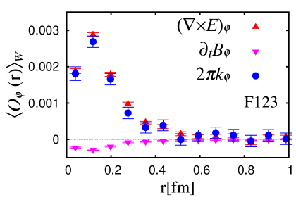
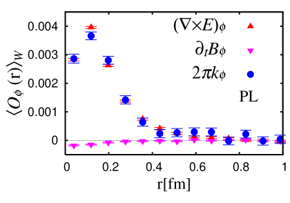
Figure 5: Curl of the Abelian electric field, the magnetic displacement current and the monopole current in the F123 (upper) and PL (lower) gauges.

To identify what squeezes the Abelian electric field, let us study the Abelian (dual) Ampère law $\vec{\nabla}\times\vec{E}=\partial_{t}\vec{B}+2\pi\vec{k}$ . In Fig. 5, we show the profile of each term in the F123 and the PL gauges, where only the non-vanishing azimuthal components are plotted. We find that the curl of electric field $\vec{\nabla}\times\vec{E}$ is reproduced by the monopole current $2\pi\vec{k}$, while the magnetic displacement current $\partial_{t}\vec{B}$ gives only small contribution. The magnitude of the profile depends on the gauge, but the qualitative feature is quite similar in both gauges. Note that this behavior is consistent with that in the MA gauge Suzuki:2004dw .

It is important to note that the space-like monopole current is responsible for squeezing the electric field in the PL gauge. This suggests that the monopoles defined on the lattice do not necessarily correspond to ’t Hooft’s Abelian monopoles tHooft:1981ht , where the latter is due to the degeneracy points of eigenvalues of some adjoint operators and they are always time-like in the PL gauge Chernodub:2003mm . Rather, if the monopoles we observe on the lattice do not exactly correspond to the ’t Hooft monopoles, the role of monopoles for the Abelian confinement mechanism can be gauge independent, and indeed, the above results seem to support such an expectation.

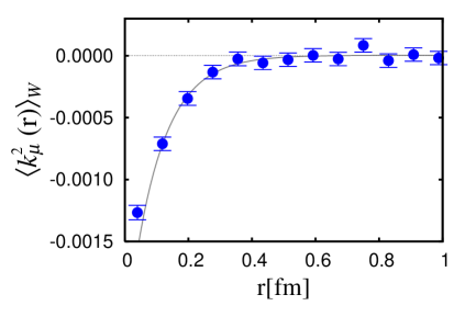
Figure 6: The profile of the squared monopole density $\langle k_{\mu}^{2}(r)\rangle_{W}$ in the PL gauge for $W(5a,5a)$. The solid line denotes the fitting curve to the function $g(r)$.

Finally, let us briefly discuss the type of the dual superconductor vacuum. For this purpose it is important to evaluate the coherence length $\xi$ as well as the penetration length $\lambda$. The ratio of these two length scales, the GL parameter $\kappa=\lambda/\xi$, classifies the vacuum type. $\sqrt{2}\kappa=1$ corresponds to the border between the type I and the type II vacua. As demonstrated in Ref. Chernodub:2005gz we may extract $\xi$ by fitting the profile of the squared monopole density $\langle k_{\mu}^{2}(r)\rangle_{W}$ to a functional form $g(r)=c^{\prime}_{1}\exp(-\sqrt{2}r/\xi)+c^{\prime}_{0}$. For the operator $k_{\mu}^{2}$ the connected correlator is reduced to the disconnected one and here we evaluate the latter. In Fig. 6, we show the profile in the PL gauge for $W(5a,5a)$. We obtain a similar behavior in the SPL gauge. However, we cannot identify the profile in the F12 and the F123 gauges within statistics, which is probably due to contamination from many ultraviolet monopoles. In Table 2, we summarize the coherence length in the SPL and the PL gauges as well as that in the MA gauge for comparison. The value of the GL parameter looks consistent with each other. However, we note that the value may not be definite since the Wilson loop size adopted here is still small and further systematic studies are required. What we can conclude here is that the vacuum type of SU(2) gluodynamics is not far from the border.

In conclusion, we have observed a clear signal of Abelian dominance in the confining part of the static potential in local unitary gauges for the first time. The structure of the flux-tube profile in these gauges strongly support a gauge-independent role of monopoles in the Abelian confinement scenario. The study of Abelian confinement mechanism without performing any gauge fixing is in progress and the result will be published elsewhere.

The authors thank to M. Polikarpov, V. Zakharov, M. Chernodub, V. Bornyakov and G. Schierholz for fruitful discussions. The numerical simulations of this work were done using RSCC computer clusters in RIKEN and SX5 at RCNP of Osaka University. The authors would like to thank RIKEN and RCNP for their support of computer facilities. T.S. is supported by JSPS Grant-in-Aid for Scientific Research on Priority Areas 13135210.

References

- (1) K. Devlin, The millennium problems : the seven greatest unsolved mathematical puzzles of our time,Basic Books, New York (2002).
- (2) G. ’t Hooft, in Proceedings of the EPS International, edited by A. Zichichi, p. 1225, 1976.
- (3) S. Mandelstam, Phys. Rept. 23, 245 (1976).
- (4) A. A. Abrikosov, Sov. Phys. JETP 5, 1174 (1957).
- (5) H. B. Nielsen and P. Olesen, Nucl. Phys. B61, 45 (1973).
- (6) N. Seiberg and E. Witten, Nucl. Phys. B426, 19 (1994), hep-th/9407087.
- (7) G. ’t Hooft, Nucl. Phys. B79, 276 (1974).
- (8) A. M. Polyakov, Nucl. Phys. B120, 429 (1977).
- (9) G. ’t Hooft, Nucl. Phys. B190, 455 (1981).
- (10) Z. F. Ezawa and A. Iwazaki, Phys. Rev. D25, 2681 (1982); T. Suzuki, Prog. Theor. Phys. 80, 929 (1988); S. Maedan and T. Suzuki, Prog. Theor. Phys. 81, 229 (1989).
- (11) T. Suzuki, Prog. Theor. Phys. 69, 1827 (1983).
- (12) A. S. Kronfeld, M. L. Laursen, G. Schierholz, and U. J. Wiese, Phys. Lett. B198, 516 (1987).
- (13) A. S. Kronfeld, G. Schierholz, and U. J. Wiese, Nucl. Phys. B293, 461 (1987).
- (14) T. Suzuki, Nucl. Phys. Proc. Suppl. 30, 176 (1993).
- (15) M. N. Chernodub and M. I. Polikarpov, in ”Confinement, Duality and Nonperturbative Aspects of QCD”, edited by P. van Baal, p. 387, Cambridge, 1997, Plenum Press.
- (16) V. Singh, D. A. Browne, and R. W. Haymaker, Phys. Lett. B306, 115 (1993),hep-lat/9301004; G. S. Bali, C. Schlichter, and K. Schilling, Prog. Theor. Phys. Suppl. 131, 645 (1998),hep-lat/9802005; Y. Koma, M. Koma, E.-M. Ilgenfritz, T. Suzuki, and M. I. Polikarpov, Phys. Rev. D68, 094018 (2003),hep-lat/0308008; Y. Koma, M. Koma, E.-M. Ilgenfritz, and T. Suzuki, Phys. Rev. D68, 114504 (2003),hep-lat/0302006.
- (17) T. Suzuki, Prog. Theor. Phys. Suppl. 131, 633 (1998).
- (18) T. Suzuki and I. Yotsuyanagi, Phys. Rev. D42, 4257 (1990).
- (19) K. Bernstein, G. Di Cecio, and R. W. Haymaker, Phys. Rev. D55, 6730 (1997), hep-lat/9606018.
- (20) S. Ito, T. W. Park, T. Suzuki, and S. Kitahara, Phys. Rev. D67, 074504 (2003), hep-lat/0208049.
- (21) J. M. Carmona, M. D’Elia, A. Di Giacomo, B. Lucini, and G. Paffuti, Phys. Rev. D64, 114507 (2001), hep-lat/0103005.
- (22) M. Lscher and P. Weisz, JHEP 09, 010 (2001), hep-lat/0108014.
- (23) Y. Iwasaki, Nucl. Phys. B258, 141 (1985).
- (24) M. C. Ogilvie, Phys. Rev. D59, 074505 (1999), hep-lat/9806018.
- (25) S. Necco and R. Sommer, Nucl. Phys. B622, 328 (2002), hep-lat/0108008.
- (26) M. Lscher and P. Weisz, JHEP 07, 049 (2002).
- (27) T. Suzuki, K. Ishiguro, Y. Mori, and T. Sekido, Phys. Rev. Lett. 94, 132001 (2005), hep-lat/0410001.
- (28) APE, M. Albanese et al., Phys. Lett. B192, 163 (1987).
- (29) P. Cea and L. Cosmai, Phys. Rev. D52, 5152 (1995), hep-lat/9504008.
- (30) A. Di Giacomo, M. Maggiore, and S. Olejnik, Phys. Lett. B236, 199 (1990).
- (31) M. N. Chernodub et al., Phys. Rev. D72, 074505 (2005), hep-lat/0508004.
- (32) M. N. Chernodub, Phys. Rev. D69, 094504 (2004), hep-lat/0308031.