June 2007

Can we study Quark Matter

in the Quenched Approximation?

Pietro Giudice^a and Simon Hands^b

^a Dipartimento di Fisica Teorica, Università di Torino and INFN, Sezione di Torino,

via P. Giuria 1, I-10125 Torino, Italy.

^b Department of Physics, Swansea University,

Singleton Park, Swansea SA2 8PP, U.K.

Abstract

We study a quenched SU(2) lattice gauge theory in which, in an attempt to distinguish between timelike and spacelike gauge fields, the gauge ensemble $\{U_{\mu}\}$ is generated from a 3 dimensional gauge-Higgs model, the timelike link variables being “reconstructed” from the Higgs fields. The resulting ensemble is used to study quenched quark propagation with non-zero chemical potential $\mu$; in particular, the quark density, chiral and superfluid condensates, meson, baryon and gauge-fixed quark propagators are all studied as functions of $\mu$. While it proves possible to alter the strength of the inter-quark interaction by changing the parameters of the dimensionally reduced model, there is no evidence for any region of parameter space where quarks exhibit deconfined behaviour or thermodynamic observables scale as if there were a Fermi surface.

PACS: 11.15.Ha, 12.38Gc, 12.38.Mh

Keywords: quenched approximation, non-zero chemical potential

1 Introduction

Lattice QCD at non-zero quark chemical potential $\mu$ ought in principle to be much more straightforward than the corresponding problem with non-zero temperature $T$. The reason is that $\mu$ can be introduced via a local term in the Lagrangian, whereas $T>0$ is imposed via a lattice of finite extent $L_{t}a=T^{-1}$ in the temporal direction. Simulations with varying $\mu$ can therefore be performed at fixed lattice spacing $a$, so that the renormalisation factors needed for bulk thermodynamic observables such as the Karsch coefficients required to extract the physical energy density need be calculated only once, rather than for each value of $T$ studied. Moreover, the regime $\mu/T\gg 1$ relevant for the physics of the superdense matter found in neutron star cores implies lattices with large $L_{t}$, so that temporal correlators can be sampled efficiently without recourse to anisotropic lattices requiring careful callibration. This means that excitations above the ground state of the system, or more generally the nature of the spectral density function, can be studied with relative ease. Indeed, this programme has been successfully carried out in certain theories such as the NJL and related models, where both measurement of the superfluid gap in the quasiparticle spectrum at $k\approx\mu$ [1] and the identification of a phonon excitation with $\omega\propto k$ in the spin-1 meson channel [2] have proved possible.

In practice, of course, the reason this happy state of affairs has not been exploited in QCD is the notorious Sign Problem associated with most Euclidean field theories having a non-zero density of a conserved charge. In brief, for lattice QCD with $N_{f}$ quark flavors described by a Lagrangian density of the form $\bar{q}Mq$, the functional measure $\mbox{det}^{N_{f}}M(\mu)=\mbox{det}^{N_{f}}M^{*}(-\mu)$ implying that for $\mu\not=0$ the action is complex, rendering Monte Carlo importance sampling impracticable in the thermodynamic limit. Can one then at least perform lattice QCD simulations in the quenched $N_{f}\to 0$ limit, i.e. study the propagation of valence quarks with $\mu\not=0$ through a non-perturbative gluon background?

In principle the information extracted from such an approach could be at best qualitative, since (unlike the case of $T>0$) the gauge field ensemble $\{U_{\mu}\}$ can only respond to $\mu\not=0$ via virtual quark loops, so that in an orthodox quenched simulation the gluon background is that of the vacuum with zero baryon charge density. Nonetheless, such information might be valuable, for instance, in furnishing a non-perturbative definition of the Fermi surface, whose existence is assumed in most phenomenological treatments of dense matter.

In the NJL studies referred to above, the Fermi surface appears as a minimum of the dispersion relation $\omega(k)$ in the neighbourhood of the Fermi momentum $k=k_{F}$: for weakly-interacting massless quarks we expect $k_{F}\approx\mu$. Even free quark propagation at $\mu\not=0$ reveals the presence of a Fermi surface and so is not entirely trivial. For QCD however, the notion of a distinguished quark momentum is not gauge invariant, so that the identification of regions of phase space occupied by low-energy excitations may be altogether more subtle in a gauge invariant formalism.

However, as plausible as this sounds, the quenched approach has conceptual difficulties at $\mu\not=0$. In the context of a random matrix theory, Stephanov [3] showed that the quenched theory should be thought of as the $N_{f}\to 0$ limit of a QCD-like theory with not just $N_{f}$ flavors of quark $q\in{\bf 3}$ of the SU(3) gauge group but also with $N_{f}$ flavors of conjugate quark $q^{c}\in\bar{\bf 3}$. As has been known for many years [4], the extra particle content results in gauge invariant $qq^{c}$ bound states in the spectrum which in a strongly interacting theory can result in baryons degenerate with light mesons. At $\mu=0$ these extra states are usually regarded as extra pions due to the fermion species doubling resulting from the use of the manifestly real positive measure $\mbox{det}MM^{\dagger}$ required by practical fermion algorithms. The introduction of $\mu\not=0$ distinguishes baryons from mesons. A simple argument, which assumes that binding energy is a relatively small component of the energy density of bulk nuclear matter, predicts that for $\mu/T\gg 1$ there should be an onset transition from the vacuum to a ground state with quark number density $n_{q}>0$ once $\mu$ equals the mass of the lightest baryon divided by the number of quark constituents. For QCD this scale is $m_{N}/3$, where $m_{N}$ is the nucleon mass; for a theory with conjugate quarks the onset scale is $m_{\pi}/2$. Only cancellations among configurations due to a complex-valued measure $\mbox{det}M$ can ensure that the fake signal for $n_{q}>0$ vanishes in the range $m_{\pi}/2<\mu<m_{N}/3$ [5]. A recent analytic demonstration has been given, once again in the context of a random matrix model, in [6].

It is clear from these considerations that quenched calculations at $\mu\not=0$ can only be useful if the distribution of gluon fields is modified in some way to reflect high baryon density. For instance, a minimum requirement is that the timelike links $U_{0}$ are no longer drawn from the same sampling distribution as spacelike links $U_{i}$, reflecting the breakdown of Lorentz invariance due to the preferred rest frame of the background quark distribution. If the gluons were modified in some way so that color confinement no longer holds, then the role of $qq^{c}$ excitations may not be so important in determining the ground state in the quark sector, and it is at least conceivable that valence quark propagation in such a background may qualitatively resemble that of the deconfined regime of the phase diagram at $\mu/T\gg 1$ corresponding to quark matter. The focus of such a study would thus be “cold quarks in hot glue”. While there are several lines one could take, the approach we shall explore in this study is to start with the 3$d$ configurations characteristic of the deconfined phase found at $T>T_{c}$, $\mu/T\ll 1$ produced by the approach to hot gauge theory known as Dimensional Reduction (to be reviewed below in Secs. 2.1 and 2.2). In this approach all non-static modes of the gauge theory (ie. those with non-zero Matsubara frequency) are integrated out leaving a 3$d$ gauge-Higgs model describing the non-perturbative behaviour of the remaining static modes. For sufficiently large $T/T_{c}$ the model coefficients are perturbatively calculable functions of $T$, $\mu$ and $N_{f}$, and the resulting effective theory can be used to make quantitative predictions in the quark gluon plasma phase. Our goals are less ambitious and more speculative; we will use the Higgs fields of the 3$d$ theory to “reconstruct” the timelike gauge fields $U_{0}$ and hence generate (3+1)$d$ configurations of static gauge fields suitable for the study of valence quark propagation with $\mu\not=0$. At this stage we are simply trying to generate a non-confining gluon background, and in no sense claim to be developing a high density effective theory.

With gauge group SU(3) and $\mu\not=0$, the dimensional reduction (DR) machinery yields a cubic higgs self-interaction with imaginary coefficient proportional to $N_{f}$  [7], which is how the 3$d$ effective theory inherits the sign problem from (3+1)$d$ QCD. Whilst there is no reason to suppose the sampling of the model’s configuration space would be any less problematic than that of the full theory, at least the complex phase of each configuration is now expressed in terms of a local term in the action, making its calculation cheap. Moreover, since the coefficient of the complex term can be made arbitrarily small ad hoc, the effect of gradually introducing the sign problem, and the interplay of the complex phase with physical observables, could be explored. In this paper, however, we focus on the technically simpler case of gauge group SU(2). In this case the action is real for even $N_{f}$ (and the cubic DR higgs self-interaction vanishes), permitting orthodox lattice simulations with standard algorithms, e.g. [8].

QCD with gauge group SU(2), often referred to as Two Color QCD or QC₂D, has been studied at $\mu\not=0$ with lattice simulations by several groups using a variety of formulations and algorithms [5, 8, 9, 10, 11, 12]. Since $q$ and $\bar{q}$ fall in equivalent representations of the gauge group, so that in effect $q$ and $q^{c}$ are identical, hadron multiplets contain both $q\bar{q}$ mesons and $qq$, $\bar{q}\bar{q}$ baryons, which are degenerate at $\mu=0$. In the chiral limit the lightest hadrons are Goldstone bosons, and can be analysed using chiral perturbation theory ($\chi$PT) [13]. At leading order for $\mu\gg T$ a second order onset transition from vacuum to matter consisting of tightly bound diquark scalar bosons is predicted at exactly $\mu_{o}=m_{\pi}/2$. At the same point the chiral condensate $\langle\bar{q}q\rangle$ starts to fall below its vacuum value, and a non-vanishing diquark condensate $\langle qq\rangle$ develops, such that $\langle\bar{q}q\rangle^{2}+\langle qq\rangle^{2}$ remains constant. The diquark condensate spontaneously breaks U(1) baryon number symmetry, so the resulting ground state is superfluid. In the limit $\mu\to\mu_{o+}$ the matter in the ground state becomes arbitrarily dilute, weakly-interacting, and non-relativistic, and is a textbook example of Bose-Einstein condensation. This scenario was subsequently confirmed by simulations with staggered lattice fermions [5, 9]. More recent simulations have found evidence for a second transition at larger $\mu$ to a deconfined phase, as evidenced by a non-vanishing Polyakov loop [11] and by a fall in the topological susceptibility [12]. In this regime thermodynamic quantities scale according to the expectations of free field theory (also referred to as “Stefan-Boltzmann” (SB) scaling), namely $n_{q}\propto\mu^{3}$, and energy density $\varepsilon\propto\mu^{4}$ [11].

In this paper we build on our existing experience by exploring $\mu\not=0$ in quenched QC₂D. In Sec. 2 below we specify our procedure for generating (3+1)$d$ quenched SU(2) gauge configurations starting from a 3$d$ gauge-Higgs model, and review standard quark observables once $\mu\not=0$. Our results follow in Sec. 3. First we explore the quark density $n_{q}$ and the chiral $\langle\bar{q}q\rangle$ and superfluid $\langle qq\rangle$ condensates to see how the equation of state responds to attempts to render the (3+1)$d$ theory “non-confining”, and whether the behaviour predicted by $\chi$PT can be supplanted by the SB scaling expected of weakly-interacting degenerate quarks. Next we turn to spectroscopy, calculating both “normal” and “anomalous” components of the quark propagator, taking advantage of the enormous gain in statistical accuracy offered by the quenched approach. First we study the bound state spectrum in both meson and diquark sectors, finding evidence for significant mixing between the sectors at large enough $\mu$. Next, for the first time in a gauge theory, we present results for the quark propagator at $\mu\not=0$ obtained following gauge-fixing. A range of spatial momenta are sampled in an attempt to map out the quasiquark dispersion relation. While we find significant qualitative differences between strongly and weakly-interacting quarks, no signal for a Fermi surface has emerged. Our conclusions follow in Sec. 4.

2 Formulation

2.1 Reconstructing the Fourth Dimension

The quenched action we start from is the 3$d$ SU(2) gauge – adjoint Higgs model given by Eqn. (4) of Ref.[14]:

$$S_{3d} = \beta\sum_{x,i>j}\left(1-{1\over 2}\mbox{tr}U_{x,ij}\right)+2\sum_{x}\mbox{tr}(\varphi_{x}\varphi_{x})$$ (1)

$$- 2\kappa\sum_{x,i}\mbox{tr}(\varphi_{x}U_{x,i}\varphi_{x+\hat{\imath}}U_{x,i}^{\dagger})+\lambda\sum_{x}(2\mbox{tr}(\varphi_{x}\varphi_{x})-1)^{2},$$

where $\varphi\equiv{1\over 2}\varphi_{a}\tau_{a}$ is a traceless hermitian $2\times 2$ matrix representing the adjoint Higgs field. As is usual in a gauge-Higgs model, increasing $\kappa$ at sufficiently large $\beta$ takes one from a “confinement” phase with small $\langle\mbox{tr}\varphi\varphi\rangle$ to a “Higgs” phase with large $\langle\mbox{tr}\varphi\varphi\rangle$.

The action (1) is derived by dimensional reduction from a 4$d$ pure gauge SU(2) theory with non-zero temperature $T$. In continuum notation the original Lagrangian density ${\cal L}_{4}\sim(\partial_{\mu}A_{\nu})^{2}$ in terms of a gluon field with canonical mass dimension $[A]=1$. The dimensionally reduced Lagrangian is obtained by integrating over Euclidean time and discarding all non-static modes, ie. setting $\partial_{0}=0$:

$${\cal L}_{3}=\int_{0}^{1\over T}dx_{0}{\cal L}_{4}\sim{1\over T}(D_{i}A_{j})^{2}+{1\over T}(D_{i}A_{0})^{2}\equiv(D_{i}B_{j})^{2}+(D_{i}\Phi)^{2},$$ (2)

with the new fields defined by $B_{i}=T^{-{1\over 2}}A_{i}$, $\Phi=T^{-{1\over 2}}A_{0}$, $[B]=[\Phi]={1\over 2}$. When transcribing to the 3$d$ lattice action (1) we use

$$U_{i}=\exp(igaA_{i})=\exp(igaT^{1\over 2}B_{i});\;\;\;\varphi=\sqrt{a\over\kappa}\Phi,$$ (3)

with $[U]=[\varphi]=0$. The 3$d$ lattice parameters $\beta$, $\kappa$ and $\lambda$ are all dimensionless, with $\beta$ given in terms of the Yang-Mills coupling by

$$\beta={4\over{ag_{3}^{2}}}\equiv{4\over{ag^{2}T}}={4N_{\tau}\over g^{2}},$$ (4)

where it is helpful to distinguish between the dimensionful coupling $g_{3}$ of the 3$d$ theory and the dimensionless coupling $g$ of the parent hot 4$d$ theory, related via $g_{3}^{2}=g^{2}T$; in the final equality we have assumed that the 4$d$ theory is formulated on a lattice with $N_{\tau}$ time spacings.

In the DR approach to the effective description of hot field theory, the parameters $\beta$, $\kappa$ and $\lambda$ are perturbatively calculable functions of $g$, $T$ and quark chemical potential $\mu$, as outlined in [7]. The attractiveness of this approach is that effects of, say $N_{f}$ flavors of massless quark or a small quark chemical potential $\mu$ can be incorporated in the coefficient calculation, the result always being a $3d$ bosonic model which is relatively cheap to simulate. The DR provides a good effective description when the non-static modes decouple; the authors of [7, 14] claim that this is valid for $T\raisebox{-2.15277pt}{$\ \stackrel{{\scriptstyle\textstyle>}}{{\textstyle\sim}}\ $}2T_{c}$, $\mu\raisebox{-2.15277pt}{$\ \stackrel{{\scriptstyle\textstyle<}}{{\textstyle\sim}}\ $}4T$. The parameter choice employed in this study is discussed further below in Sec. 2.2.

As discussed in Sec. 1, the quenched approximation has long been considered to be inapplicable to QCD with $\mu\not=0$, because it includes unphysical light baryons formed as bound states of $q\in{\bf 3}$ and $q^{c}\in\bf{\bar{3}}$ [3, 4]. The reason these $qq^{c}$ states are light and hence distort the physics is because at $T=0$ quenched QCD configurations are in a confining phase, implying spontaneous chiral symmetry breaking. The lightest $qq^{c}$ state is degenerate with the Goldstone pion. Our goal is to study quark propagation through a non-confining quenched gluon background with $\mu\not=0$. Since chemical potential couples to quarks via the timelike component of the current $\mu\bar{\psi}\gamma_{0}\psi$, this is an inherently four-dimensional problem. In order to generate such a background we take a 3$d$ configuration generated by the DR simulation, motivated by the fact that it describes deconfining physics, and “reconstruct” the gauge field in the timelike direction following (3) via the prescription (recall $aA_{0}=aT^{1\over 2}\Phi=(a\kappa T)^{1\over 2}\varphi$):

$$U_{0}=\exp\left(ig\sqrt{\kappa\over N_{\tau}}\varphi\right)=\cos\left(\tilde{g}\sqrt{\varphi_{a}\varphi_{a}}\right)+i{{\tau_{a}\varphi_{a}}\over\sqrt{\varphi_{a}\varphi_{a}}}\sin\left(\tilde{g}\sqrt{\varphi_{a}\varphi_{a}}\right),$$ (5)

with $\tilde{g}=\sqrt{\kappa\over\beta}$. Spatial link variables $U_{i}$ are taken to be time independent and identical to their 3$d$ counterparts. The resulting model differs from DR in that it has a non-trivial electrostatic potential (ie. a spatially-varying $U_{0}$ field), but more importantly differs from real physics with $\mu\gg T$ in that there are no non-static (ie. $\partial_{0}\not=0$) modes. It is not derivable from QCD in any systematic way.

It is legitimate to ask whether excluding non-static modes from consideration is too severe an approximation to be physically reasonable. It is possible to examine this issue for degenerate quark matter interacting weakly via gluon exchange  [16]. The loop integral in the self-consistent equation for the color-superconducting gap $\Delta$ is dominated by small angle scattering between quarks at antipodal points of the Fermi sphere, diverging as $\ln\theta$ where $\theta\sim q_{0}/\mu$, $q_{0}$ being the timelike momentum of the exchanged gluon. The divergence must be cut off by some physical screening mechanism: for electric gluons this is Debye screening, resulting in a $\theta_{min}\sim g$ below which the interaction is effectively point-like; for magnetic gluons the mechanism is Landau damping resulting in $\theta_{min}\sim g^{2\over 3}q_{0}^{1\over 3}/\mu^{1\over 3}$. In the static limit $q_{0}\to 0$ magnetic gluons are thus unscreened in perturbation theory, and the resulting gap equation yields $\Delta\sim\mu\exp(-3\pi^{2}/\sqrt{2}g)$ [17]. The effect of neglecting non-static modes such as electric gluons can be shown to affect the pre-exponential factor, but not the scaling of the gap with the coupling strength. Neglect of non-static modes thus seems defensible in a weak-coupling approach to quark matter; beyond perturbation theory we have little to guide us.

A conceptual point worth stressing is that due to the different ways spacelike and timelike links are treated, there is no simple relation between spatial and temporal lattice spacings. In principle one could determine the relation empirically by comparison of correlators in different directions, and $a_{s}/a_{t}$ callibrated by matching, say, to the ratio of the physical (and $T,\mu$-dependent) Debye screening mass to a hadron mass measured at $\mu=0$. We make no attempt to follow this prescription in this exploratory study: all masses and energy scales are compared with a reference scale chosen to be the pion mass at $\mu=0$, calculated in dimensionless units as $m_{\pi}a_{t}$. This prevents us for the time being from a direct comparison with condensates such as the physically observable quark density, expressed in dimensionless units as $n_{q}a_{s}^{3}$. Note, however, that the dimensionless ratio $\mu/T$ can be expressed without ambiguity using lattice variables as $N_{\tau}\tilde{\mu}$, where $N_{\tau}$ is the temporal extent of the lattice and $\tilde{\mu}=\mu a_{t}$ is the dimensionless lattice chemical potential introduced in Eqn. (16) below.

To illustrate both the benefits and potential pitfalls of this approach it is helpful to consider rectangular Wilson loops. The spatial Wilson loop $W(r_{1},r_{2})$ clearly inherits the behaviour of the 3$d$ theory; it is known to decay with an area law [18]. Confinement in the (3+1)$d$ theory, however, is governed by the temporal loop $W(r,t)$ given by

$$W(r,t)={1\over N_{c}}\mbox{tr}P(\vec{0},0;\vec{r},0)U_{0}^{t}(\vec{r})P^{\dagger}(\vec{0},t;\vec{r},t)(U_{0}^{\dagger}(\vec{0}))^{t}.$$ (6)

Here $P$ is the path-ordered product of spacelike links connecting $\vec{0}$ to $\vec{r}$; because the configuration is static these can be written $P(\vec{0},0;\vec{r},0)=P(\vec{0},t;\vec{r},t)\equiv P$. Using (4,5) we deduce

$$W(r,t)={1\over N_{c}}\mbox{tr}Pe^{i2\tilde{g}t\varphi_{0}}P^{\dagger}e^{-i2\tilde{g}t\varphi_{r}}.$$ (7)

Now expand the exponentials as power series in $\tilde{g}$, noting that $(2\varphi)^{2}=\varphi_{a}\varphi_{a}1\kern-4.5pt1\equiv|\varphi|^{2}1\kern-4.5pt1$, and $\mbox{tr}\varphi^{n}=0$ for odd $n$, implying that odd terms vanish. The lowest non-trivial term is $O(\tilde{g}^{2})$:

$$-{{\tilde{g}^{2}t^{2}}\over 2!}\biggl{(}|\varphi_{0}|^{2}+|\varphi_{r}|^{2}\biggr{)}+{{4\tilde{g}^{2}t^{2}}\over N_{c}}\mbox{tr}(P\varphi_{0}P^{\dagger}\varphi_{r}).$$ (8)

To proceed we make some simplifying approximations. For any $\varphi\not=0$, $r>0$, the second term of (8) is proportional to $\varphi_{0}^{a}\varphi_{r}^{b}P_{\rm adj}^{ab}$; in the strong coupling limit $\beta\to 0$, strong link field fluctuations should make its expectation value very small, and hence we neglect all terms of this form. Secondly, when integrating over fluctuations of the $\varphi$ we assume translational invariance and neglect all non-Gaussian fluctuations (which should be valid as $\lambda\to 0$), so that $\langle|\varphi_{0}|^{2p}|\varphi_{r}|^{2q}\rangle\approx\langle|\varphi|^{2(p+q)}\rangle$. This also requires physical excitations of the $3d$ theory to be massive so that $\langle\varphi_{0}\varphi_{r}\rangle$ can be neglected. It is then straightforward to show that all $r$-dependence drops out and the expectation value of the $O(\tilde{g}^{2n})$ term is $(-1)^{n}(2\tilde{g}t\langle|\varphi|\rangle)^{2n}/(2\times(2n)!)$. Hence

$$\langle W(r,t)\rangle\approx\cos^{2}(\tilde{g}t\langle|\varphi|\rangle).$$ (9)

As required, the temporal Wilson loop is positive, well-behaved for $\tilde{g}t|\varphi|\ll 1$, and clearly does not obey an area law. The reconstructed (3+1)$d$ theory is thus non-confining. Note that the neglected $P\varphi P^{\dagger}\varphi$ terms always contribute to the series coefficients with the opposite sign (due to an extra factor of $i^{2}$), so that their inclusion would in effect make $\langle W\rangle$ decay less rapidly. Viewed as a function of Euclidean time $\langle W\rangle$ decays with a negative curvature; this is inconsistent with a transfer matrix with positive definite spectrum, which implies decays of the form $\sum_{i}c_{i}e^{-E_{i}t}$. Unsurprisingly, therefore, the (3+1)$d$ model violates unitarity.

2.2 Parameter Choice for the Dimensionally Reduced Model

The DR procedure for SU(N) gauge theory with $N_{f}$ flavours of fermions has been studied to two loops in [14]. The effective theory obtained is a three dimensional SU(N) adjoint Higgs theory, with the scalars corresponding to the electric gauge potential $A_{0}$ in the unreduced theory; the case with chemical potential $\mu\not=0$ is dealt with for example in Ref. [7].

The continuum action of the SU(2) adjoint Higgs model is given by [14]

$$S=\int d^{3}x\left\{\frac{1}{2}\mbox{tr}\left(F_{ij}F_{ij}\right)+\mbox{tr}\left(D_{i}\Phi D_{j}\Phi\right)+m_{3}^{2}\mbox{tr}\left(\Phi\Phi\right)+\lambda_{3}\left[\mbox{tr}\left(\Phi\Phi\right)\right]^{2}\right\},$$ (10)

where $F_{ij}=\partial_{i}A_{j}-\partial_{j}A_{i}+ig_{3}[A_{i},A_{j}]$ and $D_{i}\Phi=\partial_{i}\Phi+ig_{3}[A_{i},\Phi]$. The physical properties of the theory are fixed by the two dimensionless ratios

$$x=\frac{\lambda_{3}}{g_{3}^{2}},\qquad y=\frac{m_{3}^{2}}{g_{3}^{4}}.$$ (11)

In the framework of DR these parameters are completely determined by $g^{2}$ and $T$ of the original four dimensional gauge theory. Since $g^{2}$ is a running coupling its value is fixed by the renormalisation scale $\Lambda_{\overline{\rm MS}}$. Choosing the renormalisation scale as in [19] and expressing $\Lambda_{\overline{\rm MS}}$ through the critical temperature $T_{c}=1.23(11)\Lambda_{\overline{\rm MS}}$ as measured on the lattice [20], it is possible to show [19] that for $N_{f}=0$

$$g_{3}^{2}=\frac{10.7668}{\ln(8.3T/T_{c})}T,\quad x=\frac{0.3636}{\ln(6.6T/T_{c})},\quad y(x)=\frac{2}{9\pi^{2}x}+\frac{1}{4\pi^{2}}+{\cal O}(x).$$ (12)

With these equations, specifying $T/T_{c}$ completely fixes the parameters $x,y$ of the reduced model. Note that the values of $x$ and $y$ corresponding to $T_{c}$ are about $x_{c}\approx 0.19$ and $y_{c}\approx 0.14$. The model exhibits two phases: a symmetric phase with full SU(2)-type confinement and a Higgs phase with residual U(1)-type confinement [21].

Simulations of the three dimensional SU(2) adjoint Higgs model showed that this theory has a phase diagram with continuously connected Higgs and confinement phases, which are partially separated by a line of first order phase transitions [19, 22]. The discretized form of the action (10) in terms of a rescaled lattice field $\varphi$ is simply our action (1). The $3d$ lattice parameters $\beta,\kappa$ and $\lambda$ are all dimensionless. The parameters of the continuum and lattice theory are related up to two loops by a set of equations [23],

$$x = \frac{\beta\lambda}{\kappa^{2}},\qquad\beta=\frac{4}{ag_{3}^{2}},$$

$$y = \frac{\beta^{2}}{8}\left(\frac{1}{\kappa}-3-\frac{2x\kappa}{\beta}\right)+\frac{\Sigma\beta}{4\pi}\left(1+\frac{5}{4}x\right)$$ (13)

$$+ \frac{1}{16\pi^{2}}\left[(20x-10x^{2})\left(\ln\left(\frac{3\beta}{2}\right)+0.09\right)+8.7+11.6x\right],$$

where $\Sigma=3.17591$. Due to the theory’s superrenormalisability, these perturbative relations are exact in the continuum limit and, based on experience, are accurate for all $\beta>6$ [14].

$T/T_{c}$	$x$	$y$	$\kappa$	$\lambda$
$1$	0.193	0.142	0.3637812	0.0028379
$2$	0.141	0.185	0.3620027	0.0020531
$3$	0.122	0.210	0.3612335	0.0017689
$5$	0.104	0.242	0.3603992	0.0015009
$10$	0.087	0.285	0.3594500	0.0012490
$100$	0.056	0.427	0.3569257	0.0007927

Table 1: The lattice parameters for $\beta=9.0$.

In Tab. 1 we report some sample lattice parameter sets obtained by calculating $x$ and $y$ according to Eqs. (12) and fixing the ratio $T/T_{c}$; then we have calculated $\kappa$ and $\lambda$ using Eqs. (13).

For gauge group SU(3) the DR theory is very similar to Eq. (10) [7]:

$$S=\int d^{3}x\left\{\frac{1}{2}\mbox{tr}F_{ij}^{2}+\mbox{tr}[D_{i},A_{0}]^{2}+m_{3}^{2}\mbox{tr}A_{0}^{2}+\lambda_{3}(\mbox{tr}A_{0}^{2})^{2}\right\},$$ (14)

where $F_{ij}=\partial_{i}A_{j}-\partial_{j}A_{i}+ig[A_{i},A_{j}]$, $D_{i}=\partial_{i}+ig_{3}A_{i}$, $F_{ij},A_{i}$, and $A_{0}$ are all traceless $3\times 3$ Hermitian matrices ($A_{0}=A_{0}^{a}T_{a}$, etc), and $g_{3}^{2}$ and $\lambda_{3}$ are the gauge and scalar coupling constants, with mass dimension one. The physical properties of the effective theory, also in this case, are determined by the dimensionless ratios

$$x=\frac{\lambda_{3}}{g_{3}^{2}},\quad y=\frac{m_{3}^{2}(\bar{\mu}_{3}=g_{3}^{2})}{g_{3}^{4}},$$ (15)

where $\bar{\mu}_{3}$ is the $\overline{MS}$ dimensional regularization scale in $3d$.

Here we note that application of DR to QCD with $N_{f}$ quark flavors and non-zero chemical potential $\mu$ results in a complex term $ig^{3}\mu{N_{f}\over{3\pi^{2}}}\mbox{tr}A_{0}^{3}$ [7], so that the DR theory inherits the complex action of the parent theory (for gauge group SU(2) $\mbox{tr}A_{0}^{3}\equiv 0$ and the action is real). In principle a term of this form could be incorporated in our approach, the advantage being that a “Sign Problem” could be introduced with arbitrarily small coefficient, and the response of observables to small phase fluctuations of the measure assessed. This gradualist approach is of course impossible in full QCD simulations.

In applications of the DR action (1) to hot gauge theory, the parameter $\beta$ is used to control the physical lattice spacing in units of $T_{c}^{-1}$, and $\kappa$ and $\lambda$ are tuned according to relations (12, 13) to specify $T$. A complication [14] is that for the $\{\beta,\kappa,\lambda\}$ parameter set appropriate for hot QCD the 3$d$ model has its true ground state in the “Higgs” phase, whereas the perturbative continuation to QCD (12) requires it to be in the “confining” phase. Fortunately the “confining” phase appears to be metastable, so that simulations started off with small $\langle\mbox{tr}\varphi\varphi\rangle$ can be used to yield physically relevant results. Once the model is extended to 4$d$ using (5) the physical meaning of the lattice parameters is no longer clear. In this exploratory study we hold $\beta,\lambda$ fixed and, with the exception of Figs. 10 and 10 below, restrict our attention to two values of $\kappa$.

2.3 Introducing Quarks with $\mu\not=0$

Henceforth we use 4$d$ configurations $\{U_{\mu}\}$ generated as outlined above as input in quenched studies using staggered fermions in the fundamental representation of SU(2), having action $S_{1}$+$S_{2}$ with

$$S_{1}={1\over 2}\sum_{x\nu}\bar{\chi}_{x}[e^{\tilde{\mu}\delta_{\nu 0}}U_{x,\nu}\chi_{x+\hat{\nu}}-e^{-\tilde{\mu}\delta_{\nu 0}}U^{\dagger}_{x-\hat{\nu},\nu}\chi_{x-\hat{\nu}}]+m\sum_{x}\bar{\chi}_{x}\chi_{x}\equiv\bar{\chi}M\chi$$ (16)

and

$$S_{2}=\sum_{x}{j\over 2}\chi^{tr}_{x}\tau_{2}\chi_{x}+{{\bar{\jmath}}\over 2}\bar{\chi}_{x}\tau_{2}\bar{\chi}_{x}^{tr}.$$ (17)

As explained above, the lattice parameter $\tilde{\mu}$ is related to the physical quark chemical potential via $\tilde{\mu}=\mu a_{t}$. Henceforth we will ignore the distinction between $a_{s},\,a_{t}$ when quoting values for parameters such as quark mass $m$ and diquark source $j$; in consequence no attempt will be made to compare these quantities with a physical scale.

The simplest observables to discuss are the chiral condensate and quark density:

$$\langle\bar{\chi}\chi\rangle={1\over 2V}\Bigl{\langle}\mbox{tr}{{\partial{\cal G}^{-1}}\over{\partial m}}{\cal G}\Bigr{\rangle};\;\;\;n_{q}={1\over 4V}\Bigl{\langle}\mbox{tr}{{\partial{\cal G}^{-1}}\over{\partial\tilde{\mu}}}{\cal G}\Bigr{\rangle},$$ (18)

where $\langle\ldots\rangle$ denotes a quenched average using the action (1), and ${\cal G}$ is the Gor’kov propagator defined below in (25). The normalisation, somewhat arbitrary in a quenched simulation, is chosen so that in the limit $\mu\to\infty$ $n_{q}$ saturates at a value of two per lattice site. The term $S_{2}$ comprising gauge invariant diquark source terms is introduced in order to discuss the possibility of diquark condensation. The Pauli matrices $\tau_{2}$ act on SU(2) color indices. While $S_{1}$ is invariant under the global U(1) rotation $\chi\mapsto e^{i\alpha}\chi$, $\bar{\chi}\mapsto\bar{\chi}e^{-i\alpha}$, $S_{2}$ is not. Defining source strengths $j_{\pm}=j\pm\bar{\jmath}$, we obtain diquark condensates

$$\langle qq_{\pm}\rangle={1\over 2V}\Bigl{\langle}\mbox{tr}{{\partial{\cal G}^{-1}}\over{\partial j_{\pm}}}{\cal G}\Bigr{\rangle}.$$ (19)

If we choose sources such that $j_{+}=j_{+}^{*}=j$, $j_{-}=0$, then the condensate forms in the “+” channel, and a massless Goldstone pole develops in the “–” channel as $j\to 0$ as confirmed by the Ward Identity

$$\sum_{x}\langle qq_{-}(0)qq_{-}(x)\rangle={{\langle qq_{+}\rangle}\over j_{+}}.$$ (20)

The numerical implementation of all these observables is identical to that for the NJL model described in [1].

3 Numerical Results

We have chosen $\beta=9.0$ sufficiently close to the continuum limit for the DR formalism to be trustworthy, and start with a point with $T=2T_{c}$ according to (12); from Table 1 this corresponds to $\kappa=0.3620027$, $\lambda=0.0020531$.

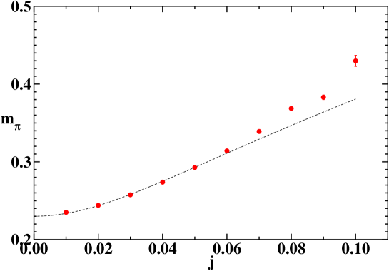
Figure 1: $m_{\pi}$ vs. $j$ from data taken on $8^{3}\times 128$ at $ma=0.05$, $\tilde{\mu}=0$ for $\beta=9.0$, $\kappa=0.362007$, $\lambda=0.0020531$.

For this parameter set, we have explored system volumes $8^{3}\times L_{t}$, with $L_{t}=16$, 32, 64 and 128. For the most part in this section we present data taken with $L_{t}=32$. However, it is important to make a precise determination of the pion mass at $\mu=0$. Fig. 1 shows data for the pion mass $m_{\pi}$ as a function of diquark source $j$ taken at $\mu=0$. The data are extrapolated to $j=0$ using a $\chi$PT-inspired form [13] $m_{\pi}(j)=m_{\pi}(0)(1+bj^{2})^{1\over 4}$ (the bare quark mass $ma=0.05$, so that the pion remains massive as $j\to 0$). We conclude $m_{\pi}a_{t}(j=0)=0.230(3)$, consistent with a measurement made exactly at $\mu=j=0$: $m_{\pi}a_{t}=0.2321(1)$. Since this scale is not too dissimilar to $L_{s}^{-1}$, we have repeated the measurement on $16^{3}\times 64$, where we find $m_{\pi}a_{t}=0.2368(3)$. The systematic error due to finite volume is significant, but small enough at 2% to be acceptable for this exploratory study.

3.1 Equation of State

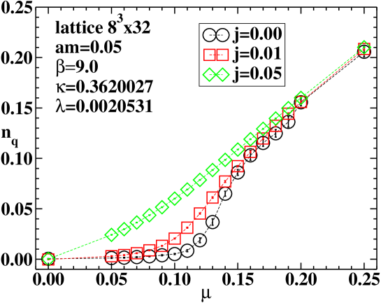
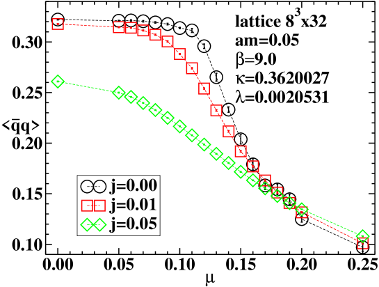
Figure 2: $n_{q}$ vs. $\tilde{\mu}$ for various $j$ using the same $\{\beta,\kappa,\lambda\}$.

Figure 3: $\langle\bar{q}q\rangle$ vs. $\tilde{\mu}$ for various $j$ using the same $\{\beta,\kappa,\lambda\}$.

In Figs. 3 and 3 we plot quark density $n_{q}$ and chiral condensate $\langle\bar{q}q\rangle$ as functions of $\mu$ for various $j$, this time on a $8^{3}\times 32$ lattice, with $0\leq\mu/T\leq 8$. The bare quark mass throughout this study was set to $ma=0.05$. To confirm freedom from finite volume effects we also performed test simulations with $L_{s}=4,8,16,32$ and $L_{t}=16,32,64$. There is a transition at $\tilde{\mu}\approx 0.12$, becoming more abrupt as $j\to 0$, from a phase with $n_{q}=0$, $\langle\bar{q}q\rangle$ constant to one in which $n_{q}$ increases approximately linearly with $\mu$ and $\langle\bar{q}q\rangle\propto\mu^{-2}$. This is in complete accordance with the scenario described by $\chi$PT in which as $\mu$ increases at $T\approx 0$ there is a transition at $\mu_{c}=m_{\pi}/2$ from the vacuum to a weakly-interacting Bose gas formed from scalar diquarks (Cf. Figs. 4 and 5 of Ref. [13]). The diquarks are supposed to Bose-condense to form a superfluid condensate; on a finite system this must be checked at $j\not=0$ using the $\langle qq_{+}\rangle$ observable of (19). Fig. 5 shows a compilation of $\langle qq_{+}\rangle$ data as a function of $j$ for $\mu$ rising from zero up to $\tilde{\mu}=0.25$, the condensate increasing monotonically with $\mu$. To determine the nature of the ground state an extrapolation $j\to 0$ is needed. We have used a cubic polynomial for data with $0.02\leq ja\leq 0.1$, which may result in some systematic uncertainty in the immediate neigbourhood of the transition, but Fig. 5 confirms that once again there is an abrupt

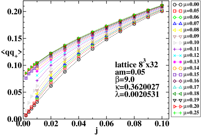
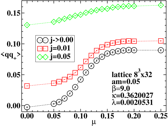
Figure 4: $\langle qq_{+}\rangle$ vs. $j$ for various $\tilde{\mu}$ using the same $\{\beta,\kappa,\lambda\}$.

Figure 5: $\langle qq_{+}\rangle$ vs. $\tilde{\mu}$ for various $j$ using the same $\{\beta,\kappa,\lambda\}$.

change of behaviour in the order parameter at $\mu\approx m_{\pi}/2$, and that the high-$\mu$ phase is superfluid.

Next we explored a parameter set corresponding to a smaller scalar “stiffness” by changing to $\kappa=0.1$ while keeping $ma=0.05$ – naively following Table 1 suggests this corresponds to a huge value of $T/T_{c}$, ie. taking us further into the deconfined phase of the hot gauge theory. Of course, whether DR-based concepts remain valid for the reconstructed theory must be addressed empirically.

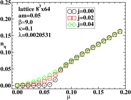
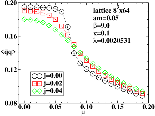
Figure 6: $n_{q}$ vs. $\tilde{\mu}$ for various $j$ at $\beta=9.0$, $\kappa=0.1$, $\lambda=0.0020531$.

Figure 7: $\langle\bar{q}q\rangle$ vs. $\tilde{\mu}$ for various $j$ using the same $\{\beta,\kappa,\lambda\}$.

This time we used a volume $8^{3}\times 64$ for the bulk observables and at $\mu=0$ determined the pion mass $m_{\pi}a_{t}=0.1377(1)$ on $8^{3}\times 128$, and $m_{\pi}a_{t}=0.1423(4)$ on $16^{3}\times 64$, showing that the finite volume error is now roughly 3%. Figs. 7 and 7 show respectively $n_{q}$ and $\langle\bar{q}q\rangle$ as functions of $\mu$ for $0\leq\mu/T\raisebox{-2.15277pt}{$\ \stackrel{{\scriptstyle\textstyle<}}{{\textstyle\sim}}\ $}12$ in the same format as previously. It is noteworthy that for $\mu>m_{\pi}/2$ $n_{q}(\mu)$ is numerically very similar to the values found at $\kappa=0.3620027$, whereas for $\mu<m_{\pi}/2$ the chiral condensate $\langle\bar{q}q\rangle$ is significantly smaller, indicative of a weaker quark – anti-quark binding at this smaller $\kappa$. As before, there is a clear discontinuity in the observables’ behaviour at $\mu_{c}\simeq m_{\pi}/2$, and the general picture is qualitatively very similar, suggesting that the $\chi$PT scenario is still applicable. Diquark binding is now also much weaker, however, as shown by the $\langle qq_{+}\rangle$ data of Fig. 8.

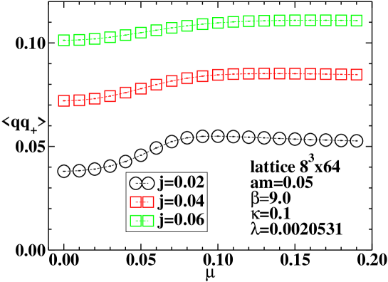
Figure 8: $\langle qq_{+}\rangle$ vs. $\tilde{\mu}$ for various $j$ using the same $\{\beta,\kappa,\lambda\}$.

Note that the source values $j$ are greater than those of Fig. 5, but the corresponding $\langle qq_{+}\rangle$ are smaller in magnitude. Since the curvature of the data as a function of $j$ is quite pronounced, a reliable extrapolation $j\to 0$ is impracticable on this system size. Indeed, inspection by eye would suggest a linear extrapolation would yield $\langle qq_{+}\rangle\simeq 0$ for all $\mu$; however, the $ja=0.02$ data do manifest some significant variation at $\mu\approx m_{\pi}/2$, suggestive that weak symmetry-breaking persists for $\mu>\mu_{c}$.

It is disappointing that we have found no qualitative change in physics as the parameters are varied – recall that the $\chi$PT model which describes the results reasonably well is based on the assumption of confinement, or at least on the presence of very tightly bound diquark states in the spectrum. To explore the parameter space more widely we focussed on a single observable, $n_{q}$, and scanned the $(\kappa,\lambda)$ plane on $8^{3}\times 16$ at five different values of $\mu$ with $\beta=9.0$, $ma=0.05$ and $ja=0.01$. The results are summarised in Figs. 10 and 10. Fig. 10 shows that except

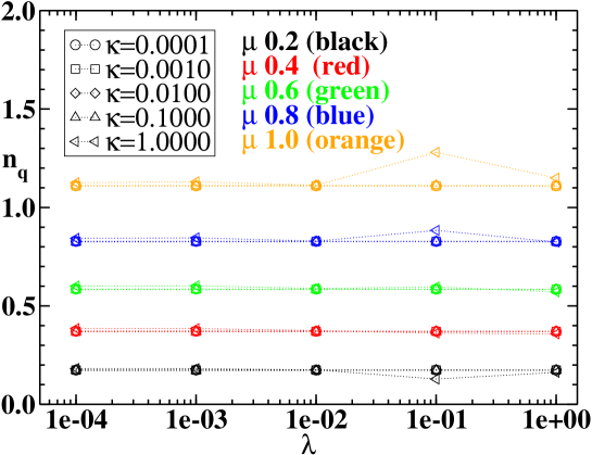
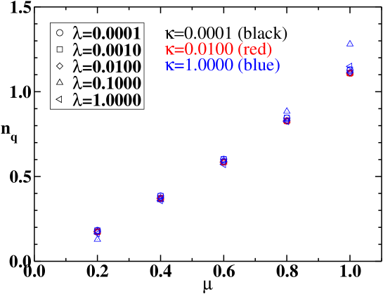
Figure 9: $n_{q}$ vs. $\lambda$ for various $\tilde{\mu}$, $\kappa$. Note $n_{q}$ increases systematically with $\mu$.

Figure 10: $n_{q}$ vs. $\tilde{\mu}$ for various $\kappa$, $\lambda$.

for $\lambda=0.1$ the results for fixed $\mu$ are practically independent of $\kappa$ (shown by the overlapping symbols) and of $\lambda$ (shown by the horizontal lines). Fig. 10 shows that $n_{q}$ increases linearly with $\mu$ over a wide region of parameter space, as it does for $\mu>\mu_{c}$ in Figs. 3,7. This approximate linear behaviour is once again a prediction of $\chi$PT [5, 9, 13], and is to be contrasted with the $n_{q}\propto\mu^{3}$ behaviour expected of a deconfined theory where baryons can be identified with degenerate quark states occupying a Fermi sphere of radius $k_{F}\approx\mu$. The absence of this scaling is a further reason to conclude that the reconstructed model does not describe deconfined physics.

3.2 Bosonic Spectrum

Next we report on bound state spectroscopy. Conventionally, $q\bar{q}$ bound states are referred to as mesons, and $qq$, $\bar{q}\bar{q}$ as diquark baryons and anti-baryons respectively. In a medium with spontaneously broken baryon number symmetry, however, excitations need not have a well-defined baryon number. An appropriate set of states to look at, together with gauge-invariant interpolating operators expressed in terms of staggered fermion fields, is as follows:

pion $$\bar{\chi}_{x}\varepsilon_{x}\chi_{x};$$ (21)

scalar $$\bar{\chi}_{x}\chi_{x};$$ (22)

higgs $${1\over 2}(\chi^{t}_{x}\tau_{2}\chi_{x}+\bar{\chi}_{x}\tau_{2}\bar{\chi}^{t}_{x})\equiv qq_{+x};$$ (23)

goldstone $${1\over 2}(\chi^{t}_{x}\tau_{2}\chi_{x}-\bar{\chi}_{x}\tau_{2}\bar{\chi}^{t}_{x})\equiv qq_{-x}.$$ (24)

Here the phase $\varepsilon_{x}=(-1)^{x_{0}+x_{1}+x_{2}+x_{3}}$, and the Pauli matrix $\tau_{2}$ acts on color indices. Pion and scalar states are related via the U(1)_ε global symmetry $\chi\mapsto e^{i\alpha\varepsilon}\chi$, $\bar{\chi}\mapsto\bar{\chi}e^{i\alpha\varepsilon}$. Analogous to chiral symmetry for continuum spinors, this is an exact symmetry of the action (16) in the limit $m\to 0$. In a phase with spontaneously broken chiral symmetry, the scalar is massive, and the pion a Goldstone mode, becoming massless as $m\to 0$. Similarly, “higgs” and “goldstone” diquark states are related via the U(1)_B baryon number rotation $\chi\mapsto e^{i\beta}\chi$, $\bar{\chi}\mapsto\bar{\chi}e^{-i\beta}$, an exact symmetry of (16,17) in the limit $j\to 0$. In a superfluid phase with $\langle qq_{+}\rangle\not=0$, the higgs is massive, and the goldstone massless in the limit $j\to 0$.

The boson correlators are constructed from the Gor’kov propagator [1]

$${\cal G}_{xy}=\left(\matrix{\bar{\jmath}\tau_{2}&M(\mu)\cr-M^{tr}(\mu)&j\tau_{2}\cr}\right)^{-1}_{xy}=\left(\matrix{A_{xy}&N_{xy}\cr\bar{N}_{xy}&\bar{A}_{xy}}\right),$$ (25)

where the $2\times 2$ (in color space) matrices $N\sim\langle\chi_{x}\bar{\chi}_{y}\rangle$ and $A\sim\langle\chi_{x}\chi_{y}\rangle$ are known as the normal and anomalous parts respectively. On a finite volume $A\equiv 0$ for $j=0$; $\lim_{j\to 0}\lim_{V\to\infty}A\not=0$ signals particle-hole mixing resulting from the breakdown of U(1)_B symmetry, and hence superfluidity. Due to SU(2) symmetries the only independent components of ${\cal G}$ are $\mbox{Re}N_{11}\equiv N$ and $\mbox{Im}A_{12}\equiv A$ and their barred counterparts, so that in practice all information from a single source can be extracted at $\mu\not=0$ using just two matrix inversions per configuration. Each of the correlators $C(t)$ constructed from the forms (21-24) receives contributions from diagrams containing both $N$ and $A$-type propagators; by construction, however, they remain symmetric under $t\mapsto-t$ even once $\mu\not=0$. Note also that in this quenched treatment contributions to the mesons from disconnected $N$ loops and to the diquarks from disconnected $A$ loops are neglected.

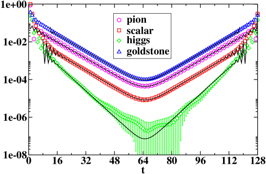
Figure 11: Timeslice propagators of various bosonic bound states at $\tilde{\mu}=0.25$ on a $8^{3}\times 128$ lattice at $\beta=9.0$, $\kappa=0.3620027$, $\lambda=0.0020531$, $ma=0.05$, $ja=0.02$.

Fig. 11 shows all four timeslice correlators evaluated on a $8^{3}\times 128$ lattice with parameter set $\beta=9.0$, $\kappa=0.3620027$ and $\lambda=0.0020531$. The chemical potential $\tilde{\mu}=0.25$, ie. above the critical $\tilde{\mu}_{c}$ required to enter the superfluid phase. The quark bare mass $ma=0.05$ and diquark source $ja=\bar{\jmath}a=0.02$. All four channels yield clear signals for single particle bound states, the higgs being the noisiest.

Like any meson constructed from staggered fermions, the correlators in principle describe two states and must be fitted using the form

$$C(t)=A[e^{-mt}+e^{-m(L_{t}-t)}]+B[e^{-Mt}+(-1)^{t}e^{-M(L_{t}-t)}].$$ (26)

where $m$ and $M$ denote the masses of states with opposite parities. Fits to (26), where positive, are shown by solid lines in Fig. 11. In most cases we find $M\gg m$; however for $\mu>\mu_{c}$ the pion correlator has a distinct “saw-tooth” shape, and in fact the fit yields $m_{\pi}>M_{b1}$, where $\pi$ denotes the usual pseudoscalar pion, and $b1$ a state of opposite parity, which must therefore be scalar (note that the logarithmic scale requires Fig. 11 to plot $|C_{\pi}(t)|$).

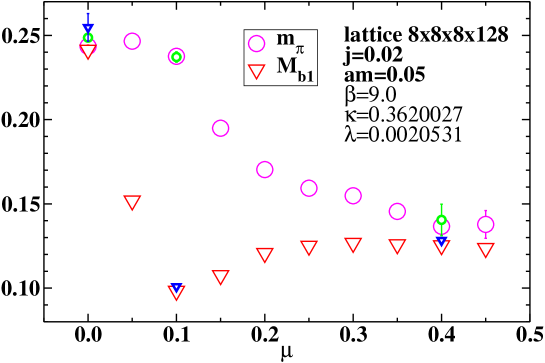
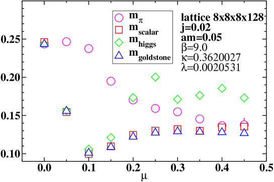
Figure 12: Mass spectrum of the pion and its parity partner as a function of $\tilde{\mu}$. Smaller symbols denote data taken on $16^{3}\times 64$.

Figure 13: Mass spectrum of various bosonic excitations as a function of $\tilde{\mu}$.

In Fig. 13 we plot $m_{\pi}$ and $M_{b1}$ against $\mu$, and in Fig. 13 the corresponding spectrum for all the states (21-24). Fig. 13 also shows $m_{\pi}$ and $M_{b1}$ as measured on a $16^{3}\times 64$ system at some representative values of $\mu$. Even for the lightest measured mass, $M_{b1}^{-1}(\tilde{\mu}=0.9)\approx 10<L_{s}$; while volume effects are statistically significant, they have no impact on the qualitative trends we now discuss. First note that all states are approximately degenerate at $\mu=0$. The equality of pion, higgs and goldstone correlators is guaranteed by SU(2) symmetry at $\mu=0$ [8], but the degeneracy of the scalar in the chirally-broken vacuum suggested by Fig. 3 can only arise as a result of meson-diquark mixing due to $j\not=0$. Next, note that the pion mass remains constant for $\mu<\mu_{c}$, where as reviewed above it is a pseudo-Goldstone boson associated with chiral symmetry breaking, and then falls once the superfluid phase is entered. This is in accordance with the predictions of $\chi$PT for the so-called “$P_{S}$” state of a theory with Dyson index $\beta_{D}=4$ [13], and has also been observed in simulations with dynamical staggered quarks in the fundamental representation of SU(2) [9]. Most of the other states, including the $b1$ in Fig. 13, show a much steeper decrease with $\mu$ for $\mu<\mu_{c}$, followed by a gentle rise to a plateau at $ma\approx 0.13$ in the superfluid phase $\mu>\mu_{c}$, precisely that expected of the goldstone state expected in the superfluid phase with diquark source $j\not=0$ (Cf. the “$Q_{I}$” state shown in Fig. 3 of [13]). The exception is the higgs, which rises more steeply to become the heaviest state at large $\mu$. We conclude (a) the breaking of degeneracy between higgs (23) and goldstone (24) states is clear supplementary evidence for the breaking of U(1)_B symmetry in the superfluid phase; (b) all states with $J^{P}=0^{+}$ including the $b1$ but except the higgs have some projection onto the Goldstone state, regardless of whether the original interpolating operator is mesonic or baryonic. It would be interesting to study this phenomenon as $j$ is varied.

3.3 Fermionic Spectrum

We have also studied the fermion spectrum, often in the context of condensed matter called the quasiparticle spectrum. Since the Gor’kov propagator ${\cal G}$ is not gauge invariant we have to specify a gauge fixing procedure. A feature of the quenched approach is that it permits large statistics to be accumulated with relatively little CPU effort. This has enabled us for the first time in a gauge theory context to study ${\cal G}$ at $\mu\not=0$, by helping to overcome the sampling problems associated with gauge fixing. We have experimented with two gauge choices: Unitary gauge $\varphi\mapsto\varphi^{\prime}=(0,0,\varphi_{3}^{\prime})$, which is implemented before the reconstruction of the 4th dimension, and is unique up to a Z₂ factor, specified by demanding $\varphi^{\prime}_{3}\geq 0$; and Coulomb gauge, implemented by maximising $\sum_{xi}\mbox{tr}(U_{x,i}+U^{\dagger}_{x-\hat{\imath},i})$, in an attempt to make the gauge fields as smooth as possible and hence improve the signal-to-noise ratio.

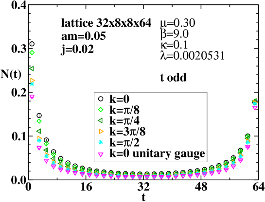
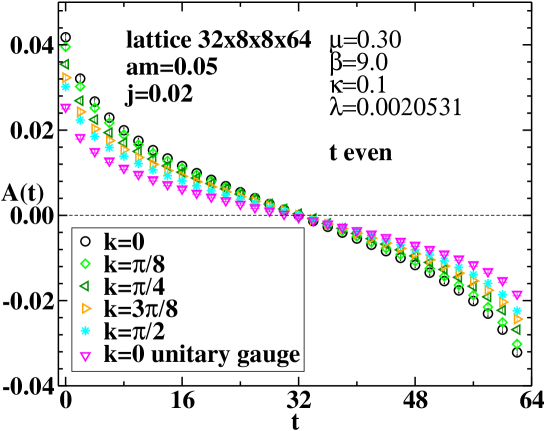
Figure 14: Normal component of the quark propagator $N(t)$ for various momenta $k$ for $\mu>\mu_{c}$.

Figure 15: Anomalous component of the quark propagator $A(t)$ for various momenta $k$ for $\mu>\mu_{c}$.

In Figs. 15 and  15 we plot respectively the normal and anomalous fermion timeslice propagators on a $32\times 8^{2}\times 64$ lattice at $\beta=9.0$, $\kappa=0.1$, $\lambda=0.0020531$, $ma=0.05$, $ja=0.0.2$ and $\tilde{\mu}=0.3$, the last value chosen to ensure $\mu>\mu_{c}$. These plots result from an analysis of 800 independent configurations. As discussed in Ref. [1], the properties of staggered lattice fermions are such that in a phase with approximate chiral symmetry, as expected for $\mu>\mu_{c}$ from Fig. 7, the numerically important contributions to $N(t)$ are from $t$ odd, and to $A(t)$ from $t$ even, and only these points are plotted. Most of the data was obtained using Coulomb gauge and differing values of the momentum $k_{x}a\in\{0,{\pi\over 16},\ldots,{\pi\over 2}\}$, though the $k_{x}=0$ data taken in unitary gauge are shown for comparison. Two features to note are that the Coulomb data is roughly twice as large as the unitary data reflecting an enhanced signal as anticipated above, and that there is little variation with $k_{x}$.

In the NJL model the quasiparticle propagator can be successfully fitted using the forms [1]

$$N(t)=Pe^{-E_{N}t}+Qe^{-E_{N}(L_{t}-t)},$$ (27)

$$A(t)=R[e^{-E_{A}t}-e^{-E_{A}(L_{t}-t)}].$$ (28)

where for $\mu\not=0$ there is no reason to expect $P=Q$, but for a well-defined quasiparticle state the equality $E_{N}=E_{A}$ should hold. Note that the anomalous amplitude $R\not=0$ is evidence for baryon number symmetry breaking, often in a condensed matter context called “particle-hole mixing”.

	Coulomb gauge	$\chi^{2}$/dof	Unitary gauge	$\chi^{2}$/dof
$E_{N}$	0.1244(7)	202	0.1651(17)	182
$E_{A}$	0.0674(13)	3.4	0.0696(15)	5.9

Table 2: Fitted mass values to the data of Figs. 15 and 15 for $k_{x}=0$.

Fits to the data of Figs. 15 and 15 are shown in Table 2, and it should be noted that only the anomalous channel fits produced an acceptable $\chi^{2}$.

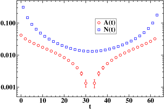
Figure 16: Comparison of the $k_{x}=0$ data of Figs. 15 and 15 on a logarithmic scale.

Some insight can be gained from Fig. 16, which compares the Coulomb gauge normal and anomalous propagators at $k_{x}=0$ on a logarithmic scale; while the fit (28) for $A(t)$ looks plausible, the normal channel never settles to a well-defined quasiparticle pole, even with $L_{t}=64$. Moreover only the anomalous channel shows any evidence of gauge independence in Tab. 2. The value of $E_{A}$ obtained is very close to $m_{\pi}/2$, indicating that at this value of $\kappa$ the pion is a weakly bound state. Another striking feature of the data is the approximate forwards-backwards symmetry of $N(t)$, implying $P\simeq Q$.

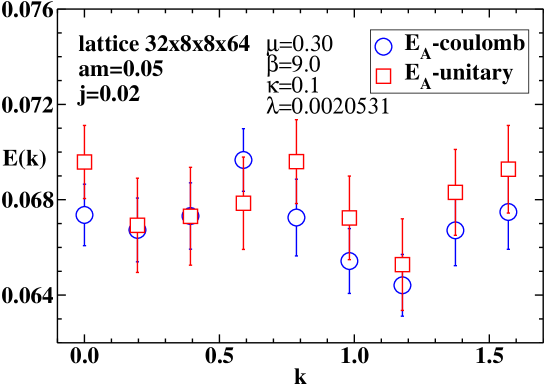
Figure 17: Dispersion relations $E_{N}(k)$ and $E_{A}(k)$.

Fig. 17 shows the dispersion relations $E_{A}(k_{x})$ for data taken on a $32\times 8^{2}\times 64$ lattice at the parameter values shown (we were unable to obtain satisfactory fits to (27) to extract $E_{N}$ for $k_{x}\not=0$). It confirms that the quasiparticle excitation energies are $k$-independent. This should be contrasted with the findings of [1], where a lattice study of the NJL model using identical formalism found $E(k)$ exhibiting a pronounced minimum at $k\approx k_{F}\approx\mu$, the Fermi momentum, evidence that the NJL model has a well-defined Fermi surface with $k_{F}\approx\mu$. One motivation for our study was to investigate to what extent the concept of a Fermi surface, which is not strictly gauge invariant, can be put on a firm empirical footing in a gauge theory. Fig. 17 shows no evidence for a Fermi surface.

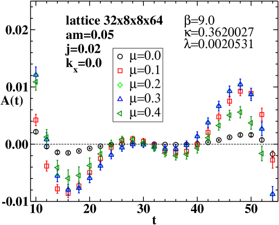
Figure 18: Close-up of $A(t)$ for $\kappa=0.3620027$ for various $\tilde{\mu}$.

The nature of the quasiparticle excitation is clarified a little at the other parameter set studied, namely $\kappa=0.3620027$ (with all other parameters unchanged). In this case our results show no evidence for any well-defined spin-${1\over 2}$ state in either normal or anomalous channels; as a result of confinement the excitation spectrum of the model seems to be saturated by the tightly bound spin-0 states of Fig. 13. Fig. 18 shows a close up of $A(t)$ for various $\mu$ values, showing the presence of an oscillatory component whose amplitude initially grows with $\mu$ (the $\tilde{\mu}=0.3$ points overlay those from $\tilde{\mu}=0.2$), but whose wavelength is roughly $\mu$-independent. The origin of the oscillation could possibly be associated with the non-unitarity of the model discussed in Sec. 2.1, but is most likely a manifestation of independent spin-${1\over 2}$ excitations being ill-defined due to confinement. We have fitted the $\kappa=0.3620027$ data to the forms

$$N(t)=Pe^{-E_{N}t}\cos(\Gamma_{N}t+\phi)+Qe^{-E_{N}(L_{t}-t)}\cos(\Gamma_{N}(L_{t}-t)+\phi),$$ (29)

$$A(t)=R[e^{-E_{A}t}\cos(\Gamma_{A}t+\phi)-e^{-E_{A}(L_{t}-t)}\cos(\Gamma_{A}(L_{t}-t)+\phi)],$$ (30)

where we interpret $E$ as the energy and $\Gamma$ as the width of a quasiparticle excitation. The results are plotted in Fig. 20.

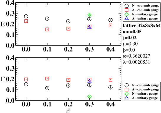
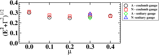
Figure 19: $E$ and $\Gamma$ vs. $\tilde{\mu}$ for $\kappa=0.3620027$ in both normal and anomalous channels.

Figure 20: $\sqrt{E^{2}+\Gamma^{2}}$ vs. $\tilde{\mu}$ for $\kappa=0.3620027$ in both normal and anomalous channels.

Most of the results are taken in Coulomb gauge, but at $\tilde{\mu}=0.3$ data from unitary gauge is also available. The results’ most striking feature is their independence of $\mu$, with $\Gamma$ of the same order of magnitude as $E$. An interesting systematic effect is that $E_{N}>E_{A}$ while $\Gamma_{N}<\Gamma_{A}$, which has motivated us in Fig. 20 to plot $\sqrt{E^{2}+\Gamma^{2}}$ vs. $\mu$. The figure has the same vertical scale as the previous two, and it is clear that the disparity between normal and anomalous channels is significantly reduced. Inspection of the $\tilde{\mu}=0.3$ data also shows that the gauge dependence of this result is O(20%) at worst. Numerically, $\sqrt{E^{2}+\Gamma^{2}}>m_{\pi}$, indicating strong quark – anti-quark binding, due to the persistence of confinement at this value of $\kappa$. Therefore we can interpret the effect of confinement as rotating the quasiparticle pole into the complex plane, the rotation angle being larger in the anomalous channel than in the normal one. It would be interesting if this feature could be reproduced by analytic methods such as self-consistent solution of Schwinger-Dyson equations.

4 Conclusion

Our attempt to alter the nature of the gluon background by changing the parameters of the 3$d$ DR gauge-Higgs model has been a partial success, in that in going from $\kappa=0.3620027$ to $\kappa=0.1$ the strength of the binding between quarks weakens significantly. The main evidence for this claim comes from the spectrum; at the smaller $\kappa$ studied quasiquarks appear to be well-defined independent degrees of freedom, whose excitation energy is to fair precision half that of the gauge-invariant pion state. At $\kappa=0.3620027$ by contrast, the quasiquark propagator exhibits a pole at complex $k$, and the resulting estimates for both energy and width of the excitation exceed the pion mass. However, in neither case is there evidence for significant departure of $n_{q}$, $\langle\bar{q}q\rangle$ and $\langle qq\rangle$ from the behaviour predicted by $\chi$PT, so that even if quarks are important degrees of freedom at $\kappa=0.1$, there is no evidence for the formation of a degenerate system signalled by SB scaling. Moreover, our attempts to measure the quasiquark dispersion relation $E(k)$ have been unsuccessful; while there is evidence for the gauge-invariance of the minimum energy or “gap” at $\kappa=0.1$, no $k$-dependence is observed. This is, of course, entirely consistent with the well-known fact that the only gauge invariant feature of a propagator is the location of its poles. We conclude that identification of a Fermi surface, supposing one existed, presents a technical challenge in any gauge theory simulation.

It is clear that our simplistic treatment, despite being manifestly gauge invariant and inclusive of non-pointlike interactions, has missed some essential component of the physics of high density. If we had first attempted the quenching programme using gauge group SU(3), the departures from the theoretical expectation of SB scaling in the large-$\mu$ limit could have been ascribed either to unexpected non-perturbative effects, or to some subtle cancellation due to the Sign Problem entirely missing from the quenched approach. For SU(2), however, orthodox simulations of full QC₂D, in which the Sign Problem is absent, yield evidence for deconfinement and SB scaling at large $\mu$ [11, 12], which our approach misses completely. We can of course speculate on which important features of the gluon background at high quark density are absent; possible candidates are non-static modes, and modes with $|\vec{k}|\approx 2k_{F}\approx 2\mu$ [15]. Sadly though, it appears to remain the case that despite its “unreasonable effectiveness” in virtually all other aspects of lattice QCD, the quenched approximation has nothing useful to tell us about the physics of high quark density.

References

- [1] S.J. Hands and D.N. Walters, Phys. Rev. D69, 076011 (2004).
-
[2]
S.J. Hands, J.B. Kogut, C.G. Strouthos and T.N. Tran, Phys. Rev.
D68, 016005 (2003);
S.J. Hands and C.G. Strouthos, Phys. Rev. D70, 056006 (2004). - [3] M.A. Stephanov, Phys. Rev. Lett. 76 (1996) 4472.
- [4] A. Gocksch, Phys. Rev. D37 (1988) 1014; Phys. Rev. Lett. 61 (1988) 2054.
-
[5]
S.J. Hands, I. Montvay, S.E. Morrison, M. Oevers, L. Scorzato and
J.I. Skullerud,
Eur. Phys. J. C17 (2000) 285;
S.J. Hands, I. Montvay, L. Scorzato and J.I. Skullerud, Eur. Phys. J. C22 (2001) 451. -
[6]
J.C. Osborn, Phys. Rev. Lett. 93, 222001 (2004);
G. Akemann, J.C. Osborn, K. Splittorff and J.J.M. Verbaarschot, Nucl. Phys. B712 (2005) 287. - [7] A. Hart, M. Laine and O. Philipsen, Nucl. Phys. B586 (2000) 443.
- [8] S.J. Hands, J.B. Kogut, M.-P. Lombardo and S.E. Morrison, Nucl. Phys. B558 (1999) 327.
- [9] J.B. Kogut, D.K. Sinclair, S.J. Hands and S.E. Morrison, Phys. Rev. D64 (2001) 094505.
-
[10]
R. Aloisio, V. Azcoiti, G. Di Carlo, A. Galante and A.F. Grillo,
Phys. Lett. B493 (2000) 189;
S. Muroya, A. Nakamura and C. Nonaka, Phys. Lett. B551 (2003) 305;
P. Giudice and A. Papa, Phys. Rev. D69, 094509 (2004);
P. Cea, L. Cosmai, M. D’Elia and A. Papa, JHEP 0702 (2007) 066;
S. Chandrasekharan and F.J. Jiang, Phys. Rev. D74, 014506 (2006). - [11] S.J. Hands, S. Kim and J.I. Skullerud, Eur. Phys. J. C48 (2006) 193.
- [12] B. Alles, M D’Elia and M.P. Lombardo, Nucl. Phys. B752 (2006) 124.
- [13] J.B. Kogut, M.A. Stephanov, D. Toublan, J.J.M. Verbaarschot and A. Zhitnitsky, Nucl. Phys. B582 (2000) 477.
- [14] A. Hart and O. Philipsen, Nucl. Phys. B572 (2000) 243.
- [15] J. Kapusta and T. Toimela, Phys. Rev. D37 (1988) 3731.
- [16] see eg., J.B. Kogut and M.A. Stephanov, The Phases of Quantum Chromodynamics, ch. 9.2 (Cambridge University Press, 2004).
- [17] D.T. Son, Phys. Rev. D 59 (1999) 094019.
-
[18]
C. Borgs, Nucl. Phys. B261 (1985) 455;
C. DeTar, Phys. Rev. D32 (1985) 276;
T.A. DeGrand and C.E. DeTar, Phys. Rev. D34 (1986) 2469. - [19] K. Kajantie, M. Laine, K. Rummukainen and M. Shaposhnikov, Nucl. Phys. B503 (1997) 357.
- [20] J. Fingberg, U. Heller and F. Karsch, Nucl. Phys. B392 (1993) 493.
- [21] S. Nadkarni, Nucl. Phys. B334 (1990) 559.
- [22] A. Hart, O. Philipsen, M. Teper and J. Stack, Phys. Lett. B396 (1997) 217.
- [23] M. Laine, Nucl. Phys. B451 (1995) 484.