The COMPASS Experiment at CERN

Abstract

The COMPASS experiment makes use of the CERN SPS high-intensity muon and hadron beams for the investigation of the nucleon spin structure and the spectroscopy of hadrons. One or more outgoing particles are detected in coincidence with the incoming muon or hadron. A large polarized target inside a superconducting solenoid is used for the measurements with the muon beam. Outgoing particles are detected by a two-stage, large angle and large momentum range spectrometer. The setup is built using several types of tracking detectors, according to the expected incident rate, required space resolution and the solid angle to be covered. Particle identification is achieved using a RICH counter and both hadron and electromagnetic calorimeters. The setup has been successfully operated from 2002 onwards using a muon beam. Data with a hadron beam were also collected in 2004. This article describes the main features and performances of the spectrometer in 2004; a short summary of the 2006 upgrade is also given.

CERN–PH–EP/2007-001

17 January 2007

, , , , , , , , , , , , , , , , ,, , , , , , , , , , , , , , , , , , , , , , , , , , , , , , , , , , , , , , , , , , , , , , , , , , , , , ,, , , , , , , , , , , , , , , , , , , , , , , , , , , , , , , , , , , , , , , , , , , , , , , , , , , , , , , , , , , , , , , , , , , , , , , , , , , , , , , , , , , , , , , , , , , , , , , , , , , , , , , , , , , , , , , , , , , , , , , , , , , , , , , , , , , , , , , , , , , , , , , , , , , , , , , , ,, , , , , , , , , , , , , , , , , , , , , , , , , , , , , , , , , , , , , , , , , , , , , , , , , , , , , , , , , , , , , , , , , , , ,, , , , , , , , ,, , , , , , , , , ,, , , , and , ,

1 Introduction

The aim of the COMPASS experiment at CERN [1] is to study in detail how nucleons and other hadrons are made up from quarks and gluons. At hard scales Quantum Chromodynamics (QCD) is well established and the agreement of experiment and theory is excellent. However, in the non-perturbative regime, despite the wealth of data collected in the previous decades in laboratories around the world, a fundamental understanding of hadronic structure is still missing.

Two main sources of information are at our disposal: nucleon structure functions and the hadron spectrum itself. While the spin-averaged structure functions and resulting parton distribution functions (PDF) are well determined and the helicity dependent quark PDFs have been explored during the last 15 years, little is known about the polarisation of gluons in the nucleon and the transversity PDF. In the meson sector the electric and magnetic polarisabilities of pions and kaons can shed light onto their internal dynamics. The reported glueball states need confirmation and an extension of their spectrum to higher masses is mandatory. Finally, hadrons with exotic quantum numbers and double-charmed baryons are ideal tools to study QCD.

Fixed-target experiments in this field require large luminosity and thus high data rate capability, excellent particle identification and a wide angular acceptance. These are the main design goals for the COMPASS spectrometer described in this article. The projects for the nucleon structure measurements with muon beam and for the spectroscopy measurements with hadron beams were originally launched independently in 1995 as two separate initiatives. The unique CERN M2 beam line, which can provide muon and hadron beams of high quality, offered the possibility to fuse the two projects into a single effort and to bring together a strong community for QCD studies. In the merging of the two experimental layouts many technical and conceptual difficulties had to be overcome, in particular the completely different target arrangements had to be reconciled. This process resulted in a highly flexible and versatile setup, which not only can be adapted to the various planned measurements, but also bears a large potential for future experiments.

In the following we give a brief description of the muon and hadron programmes from which the experimental requirements were deduced.

A recent review of our present knowledge of the spin structure of the nucleon can be found in Ref. [2]. The original discovery by the EMC in 1988 that the quark spins only account for a small fraction of the nucleon spin was confirmed with high precision during the 1990’s at CERN, SLAC and later at DESY. Thus the spin structure of the nucleon is not as simple as suggested by the naïve quark model, and both the gluon spin and the overall parton angular momentum are expected to contribute to the nucleon spin. Via the axial anomaly a very large gluon polarisation $\Delta G$ could mask the quark spin contribution and thus explain its smallness. The gluon polarisation can be studied in deep inelastic scattering either indirectly by the $Q^{2}$ evolution of the spin-dependent structure functions or more directly via the photon–gluon fusion process yielding a quark–antiquark pair which subsequently fragments into hadrons. A particularly clean process is open-charm production leading to $D$ mesons.

The detection of the decay $D^{0}\rightarrow K^{-}\pi^{+}$ and $\overline{D}^{0}\rightarrow K^{+}\pi^{-}$ (branching ratio: 3.8%) served as reference process for the design of the COMPASS spectrometer for the muon programme. Maximising luminosity together with large acceptance were important goals for the design. With present muon beam intensities only a polarised solid-state target with a high fraction of polarisable nucleons can provide the required luminosity. Apart from the luminosity, the beam and target polarisations and the dilution factor have to be taken into account to estimate the statistical accuracy of the measured double-spin cross section asymmetries. The measurements of quark polarisations, both longitudinal and transverse, require a large range in momentum transfer and thus in the muon scattering angle. The final layout covers an opening angle of the spectrometer of $\pm 180\,\mrad$ with a luminosity of almost $5\cdot 10^{32}/\cm^{2}/\s$.

Due to multiple scattering in the long solid-state target the production and decay vertices of $D$ mesons cannot be separated using a microvertex detector, otherwise a standard technique to improve the signal-to-noise ratio for heavy flavour production. The $D$ identification thus has to rely entirely on the kinematic charm decay reconstruction making excellent particle identification mandatory for background rejection. Over a wide kinematic range this task can only be performed using a Ring-Imaging Cherenkov detector. Essential for the optimisation of the signal-to-background ratio is also a good mass resolution implying the use of high-resolution tracking devices. A two-stage layout was adopted with a large aperture spectrometer close to the target mainly used for the momentum range of approximately $1-20\,\GeV/c$, followed by a small aperture spectrometer accepting particles with higher momenta, in particular the scattered muons. With this setup we also investigate spin structure functions, flavour separation, vector meson production, polarised $\Lambda$ physics and transverse quark distributions.

The physics aspects of the COMPASS programme with hadron beams are reviewed in detail in Ref. [3]. The observed spectrum of light hadrons shows new states which cannot be explained within the constituent quark model and which were interpreted as glueballs or hybrid states. In order to gain more insight, measurements with higher statistical accuracy in particular in the mass range beyond $2\,\GeV/c^{2}$ have to be performed. Different reactions are needed in order to unravel the nature of such states. They are either produced centrally or diffractively and thus a good coverage for the decay products over a wide kinematic range is required. Some of the key decay channels involve $\eta$ or $\eta^{\prime}$ with subsequent decays into photons. Their detection requires large-acceptance electromagnetic calorimetry. In addition, the flavour partners of the states observed are searched for using different beam particles ($\pi$, $K$, $p$). Beam intensities of up to $10^{8}$ particles per $5\,\s$ spill are needed imposing stringent requirements on the radiation hardness of the central detectors, in particular of the electromagnetic calorimeters.

The construction of the spectrometer started after the experiment approval by CERN in October 1998. Following a technical run in 2001 physics data were taken during 2002–2004 [4, 5, 6, 7]. Data taking resumed in 2006 after the 2005 shutdown of the CERN accelerators. Up to now only muon data were taken, apart from a two-week pilot run with a pion beam dedicated to the measurement of the pion polarisability via the Primakoff reaction. Hadron beam experiments are scheduled to start in 2007. Depending on the beam availability the present COMPASS physics programme will be completed around 2010. Future plans involving measurements of generalised parton distribution functions, detailed measurements of transversity and an extension of the spectroscopy studies are presently being discussed.

The following sections describe in more detail the general layout and the choice of technologies (Sec. 2), the beam line, the targets, tracking and particle identification, the triggers, readout electronics, data acquisition and detector control (Sec. 3–9). Section 10 represents a snapshot of the data processing procedures and of the spectrometer performance. The substantial detector upgrades implemented during the 2005 shutdown are described in Sec. 11. The article ends with a summary and an outlook.

Throughout this paper the following kinematic variables will be used: $E$ ($E^{\prime}$) is the energy of the incoming (scattered) muon, $M$ the nucleon mass, $m$ the muon mass, $\theta$ the muon scattering angle in the laboratory system, $Q^{2}$ the negative squared four-momentum of the virtual photon, $\nu=E-E^{\prime}$ its energy in the laboratory system, i.e. the energy loss of the muon, $y=\nu/E$ the fractional energy loss and $x_{\rm Bj}=Q^{2}/2M\nu$ the Bjorken scaling variable.

2 Layout of the spectrometer

2.1 General overview

The COMPASS physics programme imposes specific requirements to the experimental setup, as illustrated in the introduction to this article. They are: large angle and momentum acceptance, including the request to track particles scattered at extremely small angles, precise kinematic reconstruction of the events together with efficient particle identification and good mass resolution. Operation at high luminosity imposes capabilities of high beam intensity and counting rates, high trigger rates and huge data flows.

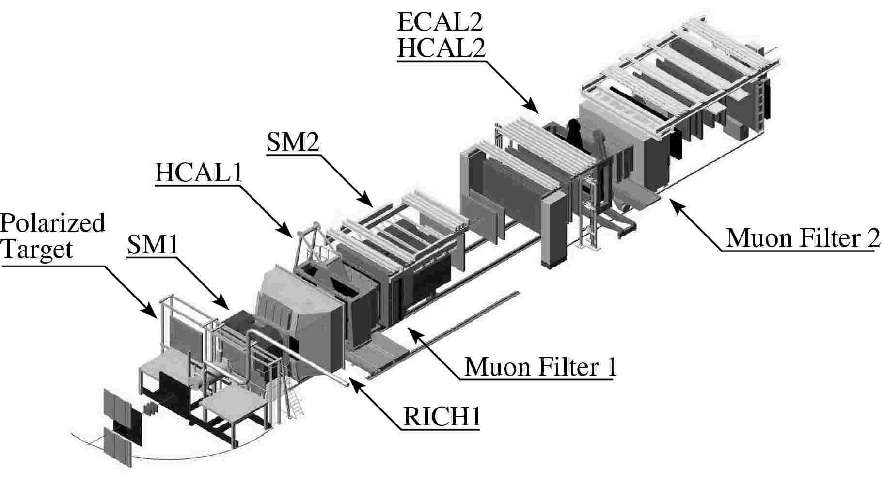
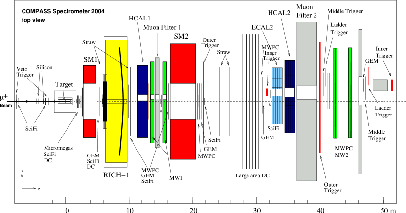
Figure 1: Compass 2004 muon setup (top) artistic view, (bottom) top view (for detector names, see text).

The basic layout of the COMPASS spectrometer, as it was used in 2004, is shown in Fig. 1. Three parts can be distinguished. The first part includes the detectors upstream of the target, which measures the incoming beam particles. The second and the third part of the setup are located downstream of the target, and extend over a total length of $50\,\m$. These are the large angle spectrometer and the small angle spectrometer, respectively. The use of two spectrometers for the outgoing particles is a consequence of the large momentum range and the large angular acceptance requirements. Each of the two spectrometers is built around an analysing magnet, preceded and followed by telescopes of trackers and completed by a hadron calorimeter and by a muon filter station for high energy muon identification. A RICH detector for hadron identification is part of the large angle spectrometer. The small angle spectrometer includes an electromagnetic calorimeter.

The flexibility required by the broad spectrum of the COMPASS physics programme has been implemented by mounting huge setup elements on rails, allowing them to be positioned at variable distances from the experimental target: the RICH, the first hadron calorimeter, the first muon filter, the second analysing magnet and the trackers fixed to it can move longitudinally on rails.

Tables 1 and 2 provide an overview of the different detectors used in COMPASS and their main parameters. The detectors are grouped according to their positions and functions in the spectrometer.

Table 1: Overview of detectors used in COMPASS, together with their respective main parameters, grouped according to their geometrical positions along the beam line (stations) and functions in the spectrometer. The first column shows the naming convention for the respective stations. The second column gives the number of detectors making up these stations, while the third column specifies the coordinates measured by the detectors. Here, e.g. $XY$ means that both projections are measured by each detector, while $X/Y$ means that only one of two coordinates $X$ or $Y$ is measured by one of the detectors. Typical values for resolutions of one detector at standard COMPASS muon beam conditions are given, where appropriate, in the sixth column. These numbers correspond to an average over all detectors of this kind in the experiment, and hence may include contributions from pile-up, magnetic fringe fields, or reconstruction inefficiencies. Here, $\sigma_{\mathrm{s}}$ denotes the r.m.s.  spatial resolution along one coordinate, $\sigma_{t}$ the r.m.s.  time resolution, $\sigma_{\mathrm{ph}}$ the single photon resolution, $\sigma_{\mathrm{ring}}$ the ring resolution. More detailed information on the respective detectors can be found in the section of the present paper specified in the last column.

Station	# of	Planes	# of ch.	Active area	Resolution	Sec.
	dets.	per det.	per det.	$X\times Y\,(\cm^{2})$
Beam detectors
BM01-04	4	$Y$	64	$6-12\times 9-23$	$\sigma_{\mathrm{s}}=1.3-2.5\,\mm$, $\sigma_{t}=0.3\,\ns$	3.3
BM05	2	$Y$	64	$12\times 16$	$\sigma_{\mathrm{s}}=0.7\,\mm$, $\sigma_{t}=0.5\,\ns$	3.3
BM06	2	$Y$	128	$12\times 16$	$\sigma_{\mathrm{s}}=0.4\,\mm$, $\sigma_{t}=0.5\,\ns$	3.3
SciFi 1,2	2	$XY$	192	$3.9\times 3.9$	$\sigma_{\mathrm{s}}=130\,\mum$, $\sigma_{t}=0.4\,\ns$	5.1.1
Silicon	2	$XYUV$	2304	$5\times 7$	$\sigma_{\mathrm{s}}=8-11\,\mum$, $\sigma_{t}=2.5\,\ns$	5.1.2
Large angle spectrometer
SciFi 3,4	2	$XYU$	384	$5.3\times 5.3$	$\sigma_{\mathrm{s}}=130\,\mum$, $\sigma_{t}=0.4\,\ns$	5.1.1
Micromegas	12	$X/Y/U/V$	1024	$40\times 40$	$\sigma_{\mathrm{s}}=90\,\mum$, $\sigma_{t}=9\,\ns$	5.2.1
DC	3	$XYUV$	1408	$180\times 127$	$\sigma_{\mathrm{s}}=190\,\mum$	5.3.1
Straw	9	$X/Y/U/V$	892	$323\times 280$	$\sigma_{\mathrm{s}}=190\,\mum$	5.3.2
GEM 1-4	8	$XY/UV$	1536	$31\times 31$	$\sigma_{\mathrm{s}}=70\,\mum$, $\sigma_{t}=12\,\ns$	5.2.2
SciFi 5	1	$XY$	320	$8.4\times 8.4$	$\sigma_{\mathrm{s}}=170\,\mum$, $\sigma_{t}=0.4\,\ns$	5.1.1
RICH-1	8	1 (pads)	10368	$60\times 120$	$\sigma_{\mathrm{ph}}=1.2\,\mrad$	6.1
					$\sigma_{\mathrm{ring}}=0.55\,\mrad$ (for $\beta=1$)
MWPC A∗	1	$XUVY$	2768	$178\times 120$	$\sigma_{\mathrm{s}}=1.6\,\mm$	5.3.3
HCAL1	1	1	480	$420\times 300$	$\Delta E/E=0.59/\sqrt{E/\GeV}\oplus 0.08$	6.3.1
MW1	8	$X/Y$	$1184/928$	$473\times 405$	$\sigma_{\mathrm{s}}=3\,\mm$	6.2.1
Small angle spectrometer
GEM 5-11	14	$XY/UV$	1536	$31\times 31$	$\sigma_{\mathrm{s}}=70\,\mum$, $\sigma_{t}=12\,\ns$	5.2.2
MWPC A	7	$XUV$	2256	$178\times 120$	$\sigma_{\mathrm{s}}=1.6\,\mm$	5.3.3
SciFi 6	1	$XYU$	462	$10\times 10$	$\sigma_{\mathrm{s}}=210\,\mum$, $\sigma_{t}=0.4\,\ns$	5.1.1
SciFi 7	1	$XY$	286	$10\times 10$	$\sigma_{\mathrm{s}}=210\,\mum$, $\sigma_{t}=0.4\,\ns$	5.1.1
SciFi 8	1	$XY$	352	$12.3\times 12.3$	$\sigma_{\mathrm{s}}=210\,\mum$, $\sigma_{t}=0.4\,\ns$	5.1.1
Straw	6	$X/Y/U/V$	892	$323\times 280$	$\sigma_{\mathrm{s}}=190\,\mum$	5.3.2
Large area DC	6	$XY/XU/XV$	500	$500\times 250$	$\sigma_{\mathrm{s}}=0.5\,\mm$	5.3.4
ECAL2	1	1	2972	$245\times 184$	$\Delta E/E=0.06/\sqrt{E/\GeV}\oplus 0.02$	6.3.3
HCAL2	1	1	216	$440\times 200$	$\Delta E/E=0.66/\sqrt{E/\GeV}\oplus 0.05$	6.3.2
MWPC B	6	$XU/XV$	1504	$178\times 90$	$\sigma_{\mathrm{s}}=1.6\,\mm$	5.3.3
MW2	2	$XYV$	840	$447\times 202$	$\sigma_{\mathrm{s}}=0.6-0.9\,\mm$	6.2.2

Table 2: Overview of trigger detectors used in COMPASS, together with their respective main parameters, grouped according to their functions in the spectrometer. The second column gives the number of detectors at this particular position, while the third column specifies the coordinates measured by these detectors. Here, $XY$ means that both projections are measured by each detector.

Det. name	# of	Planes	# of ch.	Active area
	dets.	per det.	per det.	$X\times Y\,(\cm^{2})$
Trigger hodoscopes
Inner	1	$X$	64	$17.3\times 32$
	1	$X$	64	$35.3\times 51$
Ladder	1	$X$	32	$128.2\times 40$
	1	$X$	32	$168.2\times 47.5$
Middle	1	$XY$	40/32	$120\times 102$
	1	$XY$	40/32	$150\times 120$
Outer	1	$Y$	16	$200\times 100$
	1	$Y$	32	$480\times 225$
Veto detectors
Veto 1	1		34	$250\times 320$
Veto 2	1		4	$30\times 30$
Veto BL	1		4	$50\times 50$

An introductory overview of the experimental apparatus is provided in the following: the beam spectrometer in Sec. 2.2, the large angle spectrometer in Sec. 2.3, the small angle spectrometer in Sec. 2.4, the trackers in Sec. 2.5 and the muon filters in Sec. 2.6. Setup elements specific to the physics programme with muon beam and to the first measurement performed with a hadron beam are considered in Sec. 2.7 and Sec. 2.8, respectively.

2.2 Beam telescope and beam spectrometer

The first part of the setup includes the Beam Momentum Station (BMS), located along the beam line about $100\,\m$ upstream of the experimental hall. This beam spectrometer measures the momentum of the incoming muon on an event by event base; it includes an analysing magnet and two telescopes of tracking stations formed by scintillator hodoscopes and scintillating fibre (SciFi) detectors.

A precise track reconstruction of the incident particle is provided by fast trackers located upstream of the target. There are two stations of scintillating fibres and three stations of silicon microstrip detectors. Scintillator veto counters define the beam spot size and separate the beam from the beam halo.

2.3 Large angle spectrometer

The second part, i.e. the Large Angle Spectrometer (LAS), has been designed to ensure $180\,\mrad$ polar acceptance. It is built around the SM1 magnet, which is preceded and followed by telescopes of trackers.

SM1 is a dipole magnet located $4\,\m$ downstream of the target centre. It is $110\,\cm$ long, has a horizontal gap of $229\,\cm$ and a vertical gap of $152\,\cm$ in the middle. The pole tips of the magnet are wedge-shaped with the apex of the edge facing the target, so that the tracks pointing to the target are orthogonal to the field lines. The SM1 vertical size matches the required angular acceptance of $\pm 180\,\mrad$. The main component of the field goes from top to bottom. Its field integral was measured [8] to be $1.0\,\T\m$ and corresponds to a deflection of $300\,\mrad$ for particles with a momentum of $1\,\GeV/c$. Due to the bending power of SM1, the LAS detectors located downstream of SM1 need to have an angular acceptance of $\pm 250\,\mrad$ in the horizontal plane.

The SM1 magnet is followed by a RICH detector with large transverse dimensions to match the LAS acceptance requirement, which is used to identify charged hadrons with momenta ranging from a few $\GeV/c$ to $43\,\GeV/c$. The LAS is completed by a large hadron calorimeter (HCAL1) with a central hole matching the second spectrometer acceptance. The calorimeter detects outgoing hadrons and is used in the trigger formation. The LAS is completed by a muon filter.

2.4 Small angle spectrometer

The third part of the COMPASS setup, the Small Angle Spectrometer (SAS), detects particles at small angles ($\pm 30\,\mrad$) and large momenta of $5\,\GeV/c$ and higher. Its central element is the $4\,\m$ long SM2 magnet, located $18\,\m$ downstream of the target centre and preceded and followed by telescopes of trackers.

SM2 is a rectangular shape dipole magnet with a gap of $2\times 1\,\m^{2}$ and a total field integral of $4.4\,\T\m$ for its nominal current of $4000\,\A$. As for SM1, its main field component is in the vertical direction. The SM2 magnet was used in several experiments prior to COMPASS; its magnetic field is known from previous measurements [9]. The downstream part of the SAS part includes electromagnetic and hadron calorimeters and a muon filter. Each of these elements has a hole matching the acceptance of the quasi-real photon trigger. The electromagnetic calorimeter (ECAL2) is used to detect gammas and neutral pions. The SAS hadron calorimeter (HCAL2), as well as HCAL1, is used in the trigger formation. A second muon filter is positioned at the downstream end of the spectrometer.

2.5 Tracking detectors

The particle flux per unit transverse surface varies by more than five orders of magnitude in the different regions included in the overall spectrometer acceptance. Along the beam, or close to the target, the detectors must combine a high particle rate capability (up to a few MHz/channel) with an excellent space resolution ($100\,\mum$ and better). The amount of material along the beam path has to remain at a minimum in order to minimise multiple scattering and secondary interactions. These requests are particularly severe upstream of the SM1 magnet where the incident flux is further increased because of the large number of low energy secondary particles coming from the target region. Far from the beam, the resolution constraint can be relaxed, but larger areas need to be covered. Different tracking techniques, including novel ones, are employed in regions at different distance from the beam axis, in order to match the requirements concerning rate capability, space and time resolution as well as the size of the surface to be instrumented. Different varieties of large gaseous detectors based on wire amplification are used for the regions further away from the beam, with their central regions deactivated in order not to exceed their rate capability. The near-beam and beam regions are covered by fast scintillating, gaseous and silicon tracking detectors, respectively, with active areas overlapping the dead zones of the larger detectors to guarantee efficient track reconstruction and good relative alignment.

The tracking detectors are grouped as (see also Table 1):

• Very Small Area Trackers (VSAT) - These detectors, small in size, must combine high flux capabilities and excellent space or time resolutions. The area in and around the beam is covered by eight scintillating fibres stations, and, upstream of the target, by three stations of double-sided silicon microstrip detectors. Their lateral sizes vary from $4\,\cm$ to $12\,\cm$, to take into account the beam divergence depending on the position along the beam axis.

• Small Area Trackers (SAT) - For distances from the beam larger than $2.5\,\cm$ medium size detectors, featuring high space resolution and minimum material budget are required. We use three Micromegas (Micromesh Gaseous Structure) stations, and 11 GEM (Gas Electron Multiplier) stations. Each Micromegas station is composed of four planes and has an active area of $40\times 40\,\cm^{2}$. All three stations are located between the target and the SM1 magnet. Each GEM station consists of two detectors with an active area of $31\times 31\,\cm^{2}$, each measuring two coordinates. The 11 GEM stations cover the region from the downstream side of SM1 to the far end of the COMPASS setup. Both Micromegas and GEM detectors have central dead zones with $5\,\cm$ diameter.

• Large Area Trackers (LAT) - At large angles the trackers provide good spatial resolution and cover the large areas defined by the experimental setup acceptance. In the LAS, particles emerging at large angles are tracked by three Drift Chambers (DC), one located upstream of SM1 and two immediately downstream of it. All DC have an active area of $1.8\times 1.3\,\m^{2}$ with a central dead zone of $30\,\cm$ diameter. They are followed by three stations of straw drift tubes, two upstream and one downstream of the RICH counter. Each straw station consists of two planes of size $323\times 280\,\cm^{2}$ and one plane of size $325\times 243\,\cm^{2}$, all of which have a central dead zone of $20\times 20\,\cm^{2}$. From downstream of the RICH counter to the far end of the setup the particles scattered at relatively small angles are detected by 14 multi-wire proportional chamber (MWPC) stations with active areas of $1.8\times 0.9-1.2\,\m^{2}$ and the diameters of their insensitive central zones increasing along the beam line from $16$ to $22\,\cm$. The outer region downstream of SM2 is covered by two additional straw stations of the same sizes as above, and by six large area drift chambers of $5.0\times 2.5\,\m^{2}$ active surface and $50\,\cm$ or $100\,\cm$ diameter central dead zone.

2.6 Muon filters

Identification of the scattered muons is performed by two dedicated muon filters. The design principle of a muon filter includes an absorber layer, preceded and followed by tracker stations (Muon Walls) with moderate space resolution. The absorber is thick enough to stop incoming hadrons. Muons are positively identified when a track can be reconstructed in both sets of trackers placed upstream and downstream of the absorber.

The first Muon Wall (MW1) is located at the downstream end of LAS, in front of SM2. It consists of two stations of squared drift tubes, each with an active area of $4.8\times 4.1\,\m^{2}$ and a central hole of $1.4\times 0.9\,\m^{2}$. An iron wall, $60\,\cm$ thick, is placed between the two stations.

The second Muon Wall (MW2) is installed at the very end of the SAS. The absorber is a $2.4\,\m$ thick concrete wall. The portion of the trajectory upstream of the concrete wall is reconstructed by the SAS trackers, while downstream of it there are two dedicated stations of steel drift tubes with an active surface of $4.5\times 2.0\,\m^{2}$ each.

2.7 Setup for muon beam programme

While the large majority of the spectrometer components were designed to match the needs of the entire COMPASS physics programme, some elements are specific to the measurements with muon beam, as shown in Fig. 1.

For the measurements with the muon beam the kinematic phase space covered by the spectrometer described above is expressed in terms of $Q^{2}$ and $x_{\mathrm{Bj}}$. Taking into account the geometrical acceptance of the setup, the kinematics domain covered by COMPASS for incident energies of $160\,\GeV$ extends to values of $Q^{2}$ up to $100\,(\GeV/c)^{2}$ and to values of $x_{\mathrm{Bj}}$ down to $\EE*{-5}$ as shown in Fig. 2.

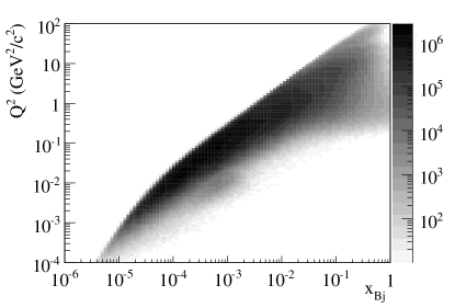
Figure 2: $x_{\mathrm{Bj}}-Q^{2}$ region covered by the COMPASS spectrometer for the $160\,\GeV/c$ muon beam.

Specific to the measurements with muon beam is the solid state polarised target. The target material is contained in two oppositely polarised target cells. The two cells are $60\,\cm$ long with $3\,\cm$ diameter, separated by a $10\,\cm$ interval. A highly homogeneous magnetic field is required to establish and preserve the target polarisation. In the years 2002-2004, the superconducting solenoid magnet previously used by the Spin Muon Collaboration (SMC) was in operation. This magnet was originally designed for inclusive deep inelastic scattering experiments only; its angular aperture of $\pm 70\,\mrad$ does not cover the whole phase space as required by the COMPASS physics programme. In 2006 it was replaced by a new, dedicated solenoid with an angular aperture of $\pm$180 mrad.

The trigger system is designed to provide a minimum bias selection of inelastic scattering events, namely to trigger on scattered muons. This is obtained by correlating the information of two stations of trigger hodoscopes formed by fast scintillator counters. In order to cope with the muon counting rates, strongly depending on the distance from the beam axis, the trigger system is formed by four subsystems, which make use of hodoscopes of different size and granularity. In addition to these hodoscopes, the hadron calorimeters are also used in order to select events with a minimum hadron energy in the final state. This criterion is particularly important to trigger on events with muons scattered at very small angles. Finally the trigger signal is completed by the beam veto counters. A stand-alone calorimetric trigger is added to cover the high $Q^{2}$ range where the scattered muon does not reach the trigger hodoscopes.

2.8 Setup for measurements with hadron beam in 2004

A first measurement with a pion beam was performed in the last weeks of the 2004 running period. The COMPASS setup was then used for a measurement of the pion electric and magnetic polarisabilities via Primakoff scattering. In this measurement the incident pion beam is scattered off a thin solid target and the scattered pion is detected in coincidence with an outgoing photon.

Several modifications were applied in order to adapt the setup to this hadron beam measurement. The large polarised target system was removed and replaced by a solid target holder, surrounded by a barrel shaped detector designed to measure low energy target fragments. This detector consists of scintillating counters inside an electromagnetic calorimeter. Two sandwiches of scintillating counters and lead foils were used to veto on photons and charged particles emitted at large angles. Two silicon microstrip telescopes were installed, with two and three stations upstream and downstream of the target, respectively, providing high angular resolution. The multiplicity information from the second telescope was used online at the event filter level. Scattering off materials along the beam path was minimised by removing the BMS and one of the scintillating fibre stations upstream of the target. For the same reason, three out of the six scintillating fibre stations downstream of the target were also removed. The size of the electromagnetic calorimeter central hole was reduced in order to fit the hadron beam size. Finally, the trigger on scattered pions was provided by a dedicated scintillator hodoscope.

3 Beam line

The CERN SPS beam line M2 can be tuned for either high-intensity positive muon beams up to $190\,\GeV/c$ or high-intensity hadron (mainly proton or mainly pion, positive or negative) beams up to $280\,\GeV/c$. Negative muon beams are also available, although with lower intensities. On request a low-energy, low-intensity tertiary electron beam can be used for test and calibration purposes. The changes between the various beam modes are fast and fully controlled from a computer terminal.

3.1 The guiding principles and optics of the muon beam

The muon beam is derived from a very intense primary proton beam, extracted from the CERN SPS at $400\,\GeV/c$ momentum, that impinges on a Beryllium target with $500\,\mm$ thickness (T6). Thinner targets can be selected for lower flux, if required. The nominal proton flux available for COMPASS is $1.2\EE{13}$ protons during $4.8\,\s$ long spills, within a $16.8\,\s$ long SPS cycle. A section of six acceptance quadrupoles and a set of three dipoles selects a high pion flux within a momentum band of up to $\pm 10\%$ around a nominal momentum up to $225\,\GeV/c$ and within a geometrical acceptance of about $3\pi\,\mu\sr$. At the production target the pion flux has a kaon contamination of about $3.6\%$. The pions are transported along a $600\,\m$ long channel, consisting of regularly spaced alternately focusing and defocusing (FODO) quadrupoles with a phase advance of $60^{\circ}$ per cell. Along this channel a fraction of the pions decay into a muon and a neutrino. Both pions and a large fraction of the muons produced in the decays are transported until the muons are focused on and the hadrons are stopped in a hadron absorber made of 9 motorised modules of Beryllium, $1.1\,\m$ long each.

The hadron absorber is located inside the aperture of a series of 3 dipole magnets, providing an upward deflection of $4.8\,\mrad$ each. These dipoles are followed by a fourth magnet, providing an additional deflection of $9.6\,\mrad$, resulting in a total deflection of $24\,\mrad$ for a good momentum separation. The dipole section is followed by a series of acceptance quadrupoles for the muons. The accepted muon beam is subsequently cleaned and momentum selected by two horizontal and three vertical magnetic collimators. All the five collimators are toroids whose gap can be adjusted to match the profile of the useful beam. The muons are transported to the surface level by a second $250\,\m$ long FODO channel. Finally the muons are bent back onto a horizontal axis by three 5 metres long dipole magnets, surrounded by 4 hodoscopes and 2 scintillating fibres planes for momentum measurement, and focused onto the polarised target. The nominal momentum of the muon section of the beam is lower than the one of the hadron section, with a maximum of $190\,\GeV/c$ with a momentum spread usually between $\pm 3\%$ and $\pm 5\%$ RMS. Typically the muon momentum is chosen to be around $90\%-94\%$ of the central hadron momentum in order to provide the best compromise between muon flux and polarisation. The final section of the beam comprises several additional bending and quadrupole magnets that fine-steer the beam on the target and, during transverse polarisation data taking, compensate for the horizontal deflection induced by the $0.5\,\T$ transverse dipole field of the polarised target.

3.2 Muon beam parameters and performance

The principles of the muon beam, as optimised for the experiments prior to COMPASS are described in more details in Ref.[10]. In order to meet the COMPASS requirements for a high intensity muon beam, the proton intensity on the Beryllium target was increased by about a factor of 2.5. Further increase was obtained by re-aligning the beam section after the production target and by retuning the openings of several collimators and scrapers. In addition, the SPS flat top (extraction time) was increased from $2\,\s$ to $4.8\,\s$, at the expense of a slight decrease of the maximum proton energy. Due to these modifications, the overall beam intensity (muons/spill) was increased by a factor of 5, and the beam duty cycle improved by more than a factor of 2.

Table 3: Parameters and performance of the $160\,\GeV/c$ muon beam.

Beam parameters	Measured
Beam momentum ($p_{\mu}$)/($p_{\pi}$)	($160\,\GeV/c$)/($172\,\GeV/c$)
Proton flux on T6 per SPS cycle	$1.2\EE{13}$
Focussed muon flux per SPS cycle	$2\EE{8}$
Beam polarisation	$(-80\pm 4)\%$
Spot size at COMPASS target ($\sigma_{x}\times\sigma_{y}$)	$8\times 8\,\mm^{2}$
Divergence at COMPASS target ($\sigma_{x}\times\sigma_{y}$)	$0.4\times 0.8\,\mrad$
Muon halo within $15\,\cm$ from beam axis	$16\%$
Halo in experiment ($3.2\times 2.5\,\m^{2}$) at $\left|x,y\right|>15\,\cm$	$7\%$

The nominal parameters of the positive muon beam are listed in Table 3. The muon momentum can be chosen between $60$ and $190\,\GeV/c$. The maximum authorised muon flux is $2\EE{8}$ muons per SPS cycle, the limitation being imposed by radio-protection guidelines. This flux can be obtained at the nominal COMPASS setting of $160\,\GeV/c$ and below, but is out of reach at higher momenta and for negative muons.

When arriving in the experimental hall, the muon beam is accompanied by a large halo, primarily composed of muons that could not be significantly deflected or absorbed. The muon halo is defined as the number of incident particles measured outside the area crossed by the nominal muon beam. The outer part of the halo is measured in the first large veto counter with a surface of $2.50\times 3.20\,\m^{2}$ and a $30\times 30\,\cm^{2}$ hole in the middle. It amounts to about $7\,\%$ of the nominal muon beam. The inner part of the halo, which also includes the tails of the beam distribution, is detected by the inner veto counters whose dimensions are $30\times 30\,\cm^{2}$ with a hole of $4\,\cm$ diameter; it represents about $16\,\%$ of the muon beam.

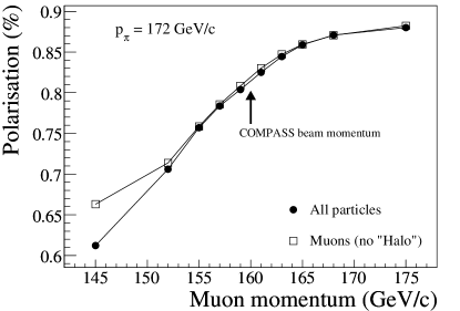
Figure 3: The muon beam polarisation (absolute value) as a function of the central muon momentum, assuming a central hadron momentum of $172\,\GeV/c$.

Due to the parity violating nature of the pion decay, the COMPASS muon beam is naturally polarised. The average beam polarisation results from the integration of all individual muon helicities over the phase space defined by the beam optics. It strongly depends on the ratio between muon and pion momenta. This is illustrated in Fig. 3, where the muon polarisation is shown as a function of the muon momentum, assuming a fixed pion momentum of $172\,\GeV/c$. The final muon polarisation value of $(-80\pm 4)\%$ in the 2004 run also includes a tiny correction due to the kaon component of the pion beam.

The statistical factor of merit of the COMPASS experiment is proportional to the beam intensity and to the square of the muon polarisation. The factor of merit is optimised for a muon polarisation of $-80\%$; the maximum allowed flux of $2\EE{8}$ muons per SPS cycle is then achieved for all momenta between $80$ and $160\,\GeV/c$. This is visible in Fig. 4 where the measured intensities are compared to a prediction from the beam simulation software. Higher polarisation values could also be reached, but at the expense of less intense muon fluxes. For standard COMPASS data taking, a beam momentum of $160\,\GeV/c$ is selected.

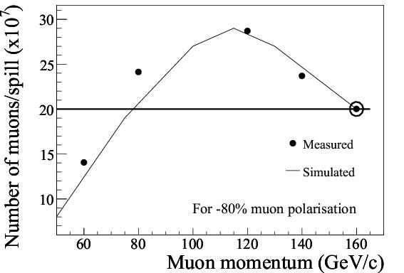
Figure 4: The maximum muon flux per SPS cycle as a function of the muon momentum, assuming a $p_{\mu}/p_{\pi}$ ratio corresponding to $-80\%$ positive muon polarisation. The points are measurements at various beam energies. The solid curve is a result from a simulation of the beam optics.

3.3 Muon beam momentum measurement

In order to make maximum use of the incident flux, the momentum spread of the beam as defined by the beam optics is large and can reach $5\%$. An accurate determination of the kinematical parameters therefore requires a measurement of the momentum of each individual muon. This is done by the Beam Momentum Station (BMS).

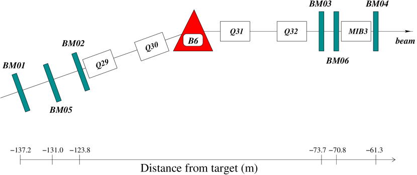
Figure 5: Layout of the Beam Momentum Station for the COMPASS muon beam.

Fig. 5 shows the detectors composing the BMS. Three consecutive dipole magnets (B6) compose the last large vertical bend ($30\,\mrad$) that brings the muon beam close to the horizontal direction before entering the experimental hall. The B6 dipoles are surrounded by a system of four quadrupoles and six beam detectors. Four of these (BM01–BM04)) are scintillator hodoscopes with horizontal scintillator strips already used in previous experiments [11]. Each hodoscope is made up of 64 elements, $5\,\mm$ high in the dispersive plane, with an overlap of a few tenths of a $\mm$ in order to avoid efficiency losses. A thickness of $20\,\mm$ along the beam ensures a large output signal. In the central regions, the scintillator strips are horizontally divided into several elements such that the particle flux per element does not exceed $1\EE{7}\,\s^{-1}$, even for the highest beam intensity. Since the beam cross section varies from one plane to another, the element length varies from $10\,\mm$ to $60\,\mm$. The readout is done using fast photomultiplier tubes (PMT). The time resolution achieved is $0.3\,\ns$.

In order to cope with the high beam current and multiple-hit environment of the COMPASS experiment, two scintillating fibre hodoscopes (BM05, BM06) were added, one in between each of the existing hodoscope pairs. These two planes provide additional redundancy in the track matching between the beam momentum station and the detectors located in front of the target, thus increasing the overall beam detection efficiency.

The design of these hodoscopes is similar to the scintillating fibre detectors used in the spectrometer (see Sec. 5.1.1). Each plane has a size of $12\,\cm$ horizontally and $16\,\cm$ vertically and is made of stacks of $2\,\mm$ round scintillating fibres. Each stack has 4 fibres along the beam direction. The overlap of two adjacent stacks is chosen such that if the traversed path in a single fibre falls below $1.4\,\mm$, the path in the adjacent fibre exceeds $1.4\,\mm$. The minimum path through the scintillator material registered in a single channel is therefore $5.6\,\mm$. The BM05 plane consists of 64 channels of two adjacent stacks each. The BM06 plane has 128 channels all made out of single stacks, in order to achieve the desired resolution in the dispersive plane. The design was chosen, such that the maximum rate per channel does not exceed $3\EE{6}\,\s^{-1}$.

Simulated beam tracks have been used to parameterize the momentum dependence of the track coordinates in these six detectors. This parameterization is used to calculate the momentum of each muon track to a precision of $\leq 1\%$. The reconstruction efficiency is $\approx 93\%$.

During event reconstruction the efficiency and the purity of the beam momentum station are further improved by using the information obtained by the tracking detectors located in front of the target. The incident tracks corresponding to the good events are reconstructed and back–propagated from the target region to the beam momentum station. The spatial correlation between the extrapolated track and the actual BMS hits is used to select among ambiguous beam candidates. If there are not enough hits in the BMS to reconstruct the momentum, a rescue algorithm is used. This algorithm relies on the determination of track angles at the first stage of BMS and at the target region. Track parts are then combined using time correlation.

3.4 Beam optics for the hadron beam

A high-intensity secondary hadron beam is obtained by moving the nine motorised hadron absorber modules out of the beam and loading settings corresponding to a single momentum all along the beam line. Up to $225\,\GeV/c$, the front end of the beam line is operated with the same optics as for the muon mode of the beam. At higher momenta a different optics is used in the acceptance quadrupoles, giving access to $280\,\GeV/c$. The beam optics is optimised for momentum resolution. The beam is composed of a (momentum dependent) mixture of pions, protons and kaons. For the tagging of individual beam particles, a pair of differential Cherenkov counters [12] (CEDAR) is foreseen in the final section of the beam. The beam optics is optimised to provide a wide and parallel beam as required for the CEDAR counters, while delivering a relatively small beam spot at the COMPASS target in the experimental hall.

Table 4: Parameters and performance of the $190\,\GeV/c$ negative hadron beam.

Beam parameters	Measured
Beam momentum	$190\,\GeV/c$
Hadron flux at COMPASS per SPS cycle	$\leq\EE*{8}$
Proportion of negative pions	$95\%$
Proportion of negative kaons	$4.5\%$
Other components (mainly antiprotons)	$0.5\%$
Typical spot size at COMPASS target ($\sigma_{x}\times\sigma_{y}$)	$3\times 3\,\mm^{2}$

The parameters of the negative hadron beam for a momentum of $190\,\GeV/c$ are listed in Table 4. For positive beams the proportions of the various particles change: at $190\,\GeV/c$ the positive beam consists of $71.5\%$ protons, $25.5\%$ pions and $3.0\%$ kaons. The maximum allowed hadron flux is $\EE*{8}$ particles per SPS cycle, limited by radiation safety rules assuming less than $20\%$ interaction length material along the beam path.

3.5 Electron beam

On request a $40\,\GeV/c$ tertiary electron beam can be provided by selecting a $100\,\GeV/c$ negative secondary beam, which impinges on a $5\,\mm$ thick lead converter, located about $50\,\m$ upstream of the hadron absorbers, which are moved out of the beam for this purpose. The downstream part of the beam line is set to $40\,\GeV/c$ negative particles, so that only the electrons that have lost $60\,\GeV$ due to Bremsstrahlung in the converter are transported to the experiment. The electron flux is typically small, of a few thousands per SPS cycle. In COMPASS the electron beam is used for an absolute calibration of the electromagnetic calorimeters.

4 Targets

4.1 Polarised target

The COMPASS muon programme aims to measure cross section asymmetries $\Delta\sigma/(2{\overline{\sigma}})$ where $\Delta\sigma$ is the difference between the cross sections of a given process for two different spin configurations and ${\overline{\sigma}}$ the spin averaged cross section. The corresponding observable counting rate asymmetry is $A_{\mathrm{obs}}=(P_{\mu}P_{\mathrm{T}}f)(\Delta\sigma/2{\overline{\sigma}})$, where $P_{\mu}$ and $P_{\mathrm{T}}$ are the beam and target polarisations, respectively, and $f$ the fraction of polarisable material inside the target. The use of a polarised target is thus mandatory and, in addition, the factors $P_{\mathrm{T}}$ and $f$ must be made as large as possible in order to optimise the statistical significance of the results. Furthermore, due to the limited muon flux, a solid state polarised target, much thicker than those commonly used in electron beams, is required.

While electron spins can be aligned in a magnetic field and give rise to a large polarisation at equilibrium for a low enough temperature, only a negligible nuclear spin polarisation can be reached. Therefore, solid state polarised targets rely on dynamic nuclear polarisation (DNP) which transfers the electron polarisation to the nuclear spins by means of a microwave field [13]. This process requires a material containing some amount of paramagnetic centres, e.g. created by irradiation, a temperature below $1\,\K$ and a strong and homogeneous magnetic field.

Deuterated lithium (⁶LiD) has been chosen as isoscalar target. This material allows to reach a high degree of deuteron polarisation ($>40\%$) and has a very favourable composition [14, 15, 16]. Indeed, since ⁶Li can be considered to a good approximation as a spin-0 ⁴He nucleus and a deuteron, the fraction of polarisable material $f$ is of the order of 0.35, taking into account also the He content in the target region. The irradiated ammonia (NH₃), which will be used as polarised proton target, has a less favourable composition ($f\approx 0.15$) but can be polarised to a higher degree ($>80\%$). Spin asymmetries are measured using a target divided in two cells, which are exposed to the same beam flux but polarised in opposite directions. In order to cancel acceptance effects which could mask the physics asymmetries, the spin directions must be frequently inverted by rotating the solenoid field. During this process, the polarisation must be maintained by a transverse field which is also needed for data taking in so-called “transverse mode”, i.e. with orthogonal directions of the beam and target polarisations. In addition, the sign of the polarisation in the target cells is inverted two or three times per year by rebuilding the polarisations with opposite microwave frequencies.

The COMPASS polarised target (see Fig. 6) has been designed to meet these requirements. It incorporates several elements previously used by the SMC experiment [17].

The superconducting solenoid (see Fig. 6,(9)) produces a $2.5\,\T$ magnetic field along the beam direction. Sixteen corrections coils (Fig. 6,(10)) are used to obtain an axial homogeneity better than $20\,\mathrm{ppm}$ in a volume $1500\,\mm$ long, and $50\,\mm$ in diameter [18]. The transverse holding field of $0.42\,\T$ is produced by a dipole coil (see Fig. 6,(12)) and deviates at most by 10% from its nominal value inside the target volume.

The ³He/⁴He dilution refrigerator is filled with liquid helium from the gas/liquid phase separator (see Fig. 6,(7)). The cold gas from the separator cools down the outer and inner vertical and horizontal thermal screens around the dilution refrigerator at nominal temperatures of $80\,\K$ and $4\,\K$, respectively. The incoming ³He gas is also cooled with cold gas from the separator. Needle valve controlled lines are used to fill the ⁴He evaporator (see Fig. 6,(6)) with liquid helium and to cool the microwave cavity (see Fig. 6,(3)). The nominal operation temperatures of the cavity and the ⁴He evaporator are $3\,\K$ and $1.5\,\K$, respectively.

A microwave cavity (Fig. 6,(3)) similar to the one previously used by SMC [17] was built. The amount of unpolarised material along the beam was minimised by reducing the thickness of the microwave stopper, and by modifying the downstream end window [19]. The $60\,\cm$ long target cells (see Fig. 6,(1),(2)) have a diameter of $3\,\cm$ and are separated by $10\,\cm$. The cells are made of a polyamide mesh in order to improve the heat exchange between the crystals and the liquid helium. They are fixed in the centre of an aramid fibre epoxy tube, which itself is fixed to the target holder isolation vacuum tube (see Fig. 6,(4)). The target cells are filled with ⁶LiD crystals of $2-4\,\mm$ size [20]; the volume between the target material crystals is filled with a mixture of liquid ³He/⁴He. The ⁶LiD mass in each target cell is $170-180\,\g$ [21], and depends on the packing factor (between 0.49 and 0.54) achieved during the filling. The isotopic dilution of deuterons with 0.5% of protons and ⁶Li with 4.2% of ⁷Li was determined by NMR measurements from the polarised target material [22]. Each cell contains five NMR coils used for the local monitoring of the polarisation.

The target material is polarised via dynamic nuclear polarisation, obtained by irradiating the paramagnetic centres with microwaves at frequencies of $70.2-70.3\,\GHz$ at 2.5 T and at temperature of about $200\,\mK$. The microwave radiation is generated with two extended interaction oscillator tubes (EIO) [17]. The density of the paramagnetic centres is of the order of 10${}^{-4}-$10^-3 per nucleus [15, 20]. An additional modulation of the microwave frequency of about $5\,\MHz$ [19, 23] helps enhancing the polarisation. A deuteron polarisation $|P|>40$% is reached within 24 hours in a $2.5\,\T$ field with a ³He flow of $80-120\,\mathrm{mmol}/\s$ in the dilution refrigerator. The maximum polarisation difference between the upstream and downstream cells $|P_{\mathrm{up}}-P_{\mathrm{down}}|>100$% is reached in five days [24], see Fig. 7.

At least once during a data taking period, the mixing chamber is filled with only ⁴He to perform the thermal equilibrium (TE) calibration of the polarisation [22] in a $2.5\,\T$ solenoid field at a constant temperature in the range $1.0-1.6\,\K$ [22]. The deuteron in the ⁶LiD material has a single $16.38\,\MHz$ NMR line about $3\,\kHz$ wide for a $2.5\,\T$ field [25]. The spin magnetisation of ⁶LiD reaches good thermal equilibrium at this temperature in about $15\,\Hour$. The polarisation of the target material is calculated from the helium temperature measured by the ³He vapour pressure [26, 27]. The intensity of the measured TE NMR signal is used to calibrate the polarisation measured during the dynamic nuclear polarisation process, when the spin system is not anymore in thermal equilibrium with the helium.

During data taking in transverse mode, the target material is kept in frozen spin mode below $90\,\mK$ and the spin direction is maintained by the $0.42\,\T$ transverse dipole field. The polarisation is reversed by exchanging the microwave frequencies of the two cells. The polarisation is measured in the longitudinal $2.5\,\T$ field at the end of each transverse data taking period of about 6 days. The relaxation rate in frozen spin mode is $(0.4-1.0)\,\%/\mathrm{d}$ in the $0.42\,\T$ field and $(0.05-0.10)\,\%/\mathrm{d}$ in the $2.5\,\T$ field.

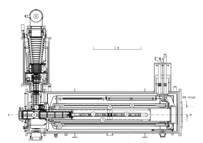
Figure 6: Side view of the COMPASS polarised target: (1) upstream target cell and (2) downstream target cell inside mixing chamber, (3) microwave cavity, (4) target holder, (5) still (³He evaporator), (6) ⁴He evaporator, (7) ⁴He liquid/gas phase separator, (8) ³He pumping port, (9) solenoid coil, (10) correction coils, (11) end compensation coil, (12) dipole coil. The muon beam enters from the left. The two halves of the microwave cavity are separated by a thin microwave stopper.

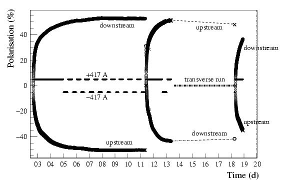
Figure 7: Typical average polarisations in the upstream and downstream target cells during 20 days of the 2004 run. After day 11, the polarisations in the target cells are reversed by changing the microwave frequencies. Data are taken in transverse mode from day 13 to day 18 and a new field reversal by microwaves is performed at the end of the period. The current of $\pm 417\,\A$ corresponds to an axial field of $2.5\,\T$.

4.2 Targets for hadron beams

During the 2004 hadron run COMPASS collected data for the measurement of the pion polarisabilities via Primakoff scattering and for the diffractive meson production studies in parallel. As the two measurements require targets with different characteristics, few solid state targets have been prepared and exchanged during the data taking. This section briefly describes the choice of target materials and geometries and their main physics motivations.

The majority of the 2004 hadron data has been collected with a target optimised for Primakoff scattering. Since this process is enhanced over the diffractive background when targets with large atomic numbers are used [28], lead was chosen as material. To study systematic effects, additional measurements of the $Z^{2}$-dependence of the Primakoff cross section using Copper and Carbon were performed (see Table 5). All targets consisted of simple discs with a diameter of $3\,\cm$, corresponding to more than 3 sigma of the beam width, while the thickness was determined by the required resolution to properly separate the electromagnetic scattering from the diffractive background. For that, the squared four-momentum transferred to the target nucleus, $t$, should be measured with a precision better than $5\EE{-4}\,\GeV^{2}/c^{2}$. The largest contribution to the uncertainty on $t$ comes from the multiple scattering in the target, allowing for a maximum thickness of about 0.5 radiation lengths.

Table 5: List of available target materials for the Primakoff and diffractive measurements. Here, $X_{0}$ denotes the radiation length and $\lambda_{\mathrm{I}}$ the nuclear interaction length.

Material	Thickness $x$	$x/X_{0}$	$x/\lambda_{\mathrm{I}}$
Lead	$3\,\mm$ ($2\,\mm+1\,\mm$ segmented)	0.53	0.029
Copper	$3.5\,\mm$	0.24	0.037
Carbon	$23\,\mm$	0.12	0.086

The study of diffractively produced hybrid mesons requires targets with low atomic numbers, such as liquid hydrogen or paraffin, to minimise the multiple scattering. On the other hand, the requirement of running the polarisability and hybrid meson programmes in parallel excluded the use of hydrogen targets. As a compromise the Carbon target has been also used for the diffractive scattering studies.

Both measurement imply a small energy transfer. In order to reject the hard scattering events in the offline analysis, the targets were inserted into a barrel-shaped veto system, called Recoil Veto, that measured the recoil energy of the target fragments produced in the reaction. The Recoil Veto consists of an inner cylindrical layer of 12 scintillator strips, with a diameter of $\sim 10\,\cm$, surrounded by an outer layer of 96 lead glass blocks. The recoil energy is measured from the combined information of the energy loss in the scintillator strips and the Cherenkov light produced in the lead glass blocks. The target material is placed at the centre of the Recoil Veto with a lightweight support made of foam.

5 Tracking detectors

The tracking system of COMPASS comprises many tracking stations, distributed over the entire length of the spectrometer. Each tracking station consists of a set of detectors of the same type, located at approximately the same $z$-coordinate along the beam. In a station, the trajectory of a charged particle is measured in several projections transverse to the beam direction in order to reduce ambiguities. In the following we use the terms $X$- and $Y$-plane to designate the group of channels within a station measuring the horizontal and vertical coordinates, respectively, of the particle penetration point. Similarly, the terms $U$- and $V$-plane describe all channels measuring projections onto axes rotated clockwise and anticlockwise, respectively, with respect to the $x$-axis. Note that the dipole magnets bend the particle trajectories in the horizontal plane. Many different detector technologies of varying rate capability, resolution, and active area are in use, dictated by the increasing particle rates closer to the beam axis, and by the spectrometer acceptance.

Section 5.1 describes the Very Small Area Trackers (VSAT), which cover the beam region up to a radial distance of $2.5$ - $3\,\cm$. The very high rate of beam particles in this area (up to about $\EE*{5}\,\s^{-1}\mm^{-2}$ in the centre of the muon beam) requires excellent time or position resolution of the corresponding detectors in order to identify hits belonging to the same track. Scintillating fibres (see Sec. 5.1.1) and silicon microstrip detectors (see Sec. 5.1.2) fulfil this task.

The intermediate region at a radial distance of $2.5\,\cm$ to $30$ - $40\,\cm$ is covered by the Small Area Trackers (SAT, see Sec. 5.2), and is the domain of micropattern gas detectors. Here, two novel devices – Micromegas (see Sec. 5.2.1) and GEM detectors (see Sec. 5.2.2)– are employed successfully for the first time in a large-scale particle physics experiment. These detectors combine high rate capability (up to about $\EE*{4}\,\s^{-1}\mm^{-2}$) and good spatial resolution (better than $100\,\mum$) with low material budget over fairly large sizes.

The reduced flux in the outermost regions, covered by the Large Area Tracker (LAT, see Sec. 5.3), allows the use of drift chambers (5.3.1, see Sec. 5.3.4), straw tube chambers (see Sec. 5.3.2), and multiwire proportional counters (see Sec. 5.3.3).

5.1 Very small area trackers

5.1.1 Scintillating fibre detectors

The purpose of scintillating fibre (SciFi) detectors in the COMPASS experiment is to provide tracking of incoming and scattered beam particles as well as of all other charged reaction products in and very near the centre of the primary beam.

As the hit rate can reach $3\EE{6}\,\s^{-1}$ per fibre in the centre of the muon beam, hits can be assigned to the corresponding track by time correlation only, whereas spatial correlation would be far too ambiguous. Time correlation is also used to link the incoming muon with the scattered muon track, as well as with the trigger and the information from the beam momentum station.

For the muon program, a total of eight SciFi detector stations are used. Two pairs of stations are placed upstream (no. 1, 2) and downstream (no. 3, 4) of the target, two more pairs upstream (no. 5, 6) and downstream (no. 7, 8) of the second spectrometer magnet (SM2). The main parameters of the different stations are given in Table 6.

Table 6: Parameters of SciFi stations in COMPASS. Column 3 specifies the number of fibre layers per projection, columns 4 and 7 give the size of the square active area and the number of channels for each projection, respectively. Column 8 lists the thickness of the respective station in units of radiation lengths ($X_{0}$).

No.	Proj.	# of	Size	Fibre ø	Pitch	# of ch.	Thickness
		layers	($\cm^{2}$)	($\mm$)	($\mm$)		($X_{0}$)
1,2	$X,Y$	14	$3.9^{2},3.9^{2}$	0.5	0.41	$96,96$	$1.64\%$
3,4	$X,Y,U$	14	$5.3^{2},5.3^{2},5.3^{2}$	0.5	0.41	$128,128,128$	$2.46\%$
5	$X,Y$	12	$8.4^{2},8.4^{2}$	0.75	0.52	$160,160$	$2.1\%$
6	$X,Y,U$	8	$10.0^{2},10.0^{2},12.3^{2}$	1.0	0.70	$143,143,176$	$2.79\%$
7	$X,Y$	8	$10.0^{2},10.0^{2}$	1.0	0.70	$143,143$	$1.86\%$
8	$X,Y$	8	$12.3^{2},12.3^{2}$	1.0	0.70	$176,176$	$1.86\%$

In total the eight SciFi stations make use more than 2500 PMT channels including about 8000 fibres. Details may be found in [29, 30]. Each station consists of at least two projections, one vertically ($Y$) and one horizontally ($X$) sensitive. Three stations (no. 3, 4, 6) comprise an additional inclined ($\sim 45^{\circ}$) projection ($U$).

In order to provide a sufficient amount of photoelectrons (at least about 20 per minimum ionising particle), several layers of fibres are stacked for each projection, the fibre axes of one layer being shifted with respect to the ones of the next layer (see Fig. 8). The overlap of fibres is chosen sufficiently large in order to avoid relying on the detection of tracks with only grazing incidence of the particles.

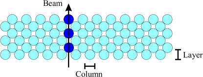
Figure 8: Fibre configuration of a SciFi plane (the actual number of fibre layers per plane is 8, 12 or 14, depending on the station).

The light output of a group of fibres lined up in beam direction (labelled “column” in Fig. 8) is collected on one photon detector channel. The number of fibres in one column is seven for stations 1–4, six for station 5, and four for stations 6–8, and is chosen to achieve the required time resolution and at the same time minimise the amount of material in the beam.

As fibre material we chose Kuraray SCSF-78MJ [31] for all SciFi stations. The scintillation light is guided by clear (not scintillating) fibres of lengths between $0.5\,\m$ and $3\,\m$. It is then detected by 16-channel multi-anode PMTs (Hamamatsu H6568 [32]) followed by fast leading edge discriminators [33] and pipelined TDCs (see Sec. 8.3.3).

Stations 1–4 have an r.m.s. spatial resolution of $130\,\mum$, station 5 of $170\,\mum$ and stations 6–8 of $210\,\mum$, with local variations which are consistent with fluctuations of the order of $10\%$ of the fibre diameter. The intrinsic detection efficiency of the SciFi stations was measured to be $\geq 99\%$. Due to occupancy in the readout in the high intensity region the efficiency is slightly lower, varying between $96\%$ and $99\%$ for the various stations.

The obtained time resolution using one plane is nearly constant for all channels. R.m.s. values between $350\,\ps$ and $450\,\ps$ were obtained for the central regions of the various planes. This can be seen from Fig. 9, where the profile of the intensity distribution in the beam region measured by one SciFi plane is shown together with the obtained time resolution.

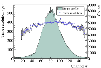
Figure 9: Time resolution (r.m.s.) of a single SciFi $Y$ plane across the beam region (triangles) together with the beam profile (histogram).

The time resolution across the plane shows a smooth curve with slightly better values in the outer region where the intensity is low.

Within the three years of operation all SciFi-detector showed a very stable operation, and there is no indication of ageing or radiation damage.

For the 2006 run an additional SciFi station was added to the setup in order to increase reconstruction efficiency of scattered muon tracks near the beam. It consists of $U$ and $V$ planes and was positioned about $110\,\cm$ upstream of SciFi station 6. Each plane of the new station has an active area of $12.3\times 6.3\,\cm^{2}$, and is read out by 96 channels. The other parameters are equal to those of the stations 7 and 8.

5.1.2 Silicon microstrip detectors

The COMPASS silicon microstrip detectors are used for the detection of the incoming muon beam track, and, for the hadron program, for vertex and track reconstruction downstream of the target. The high beam intensity in COMPASS requires a radiation hard detector design and an excellent spatial and time resolution.

The silicon wafer, optimised for high fluences, was originally designed and developed for the HERA-B experiment [34]. The $300\,\mum$ thick n-type wafer has an active area of $5\times 7\,\cm^{2}$. The 1280 readout strips on the n-side ($54.6\,\mum$ pitch) are perpendicular to the 1024 readout strips on the p-side ($51.7\,\mum$ pitch), so that with one wafer two-dimensional position information can be obtained. This reduces the material budget by a factor of two as compared to a single-sided readout.

The silicon wafer is glued with silicone glue onto a frame consisting of two L-shaped Printed Circuit Boards (L-board) forming a detector. The readout strips, which are tilted by $2.5^{\circ}$ with respect to the wafer edge, are connected via $25\,\mum$ Aluminium wire bonds and a glass pitch adapter to the front-end chips. Along two wafer edges a capillary is soldered onto the back side of the L-board and is electrically insulated by a connector of epoxy material. The capillary is flushed with gaseous nitrogen ($400\,\liter/\Hour$) to cool the front-end chips. The setup of a COMPASS silicon detector is shown in Fig. 10.

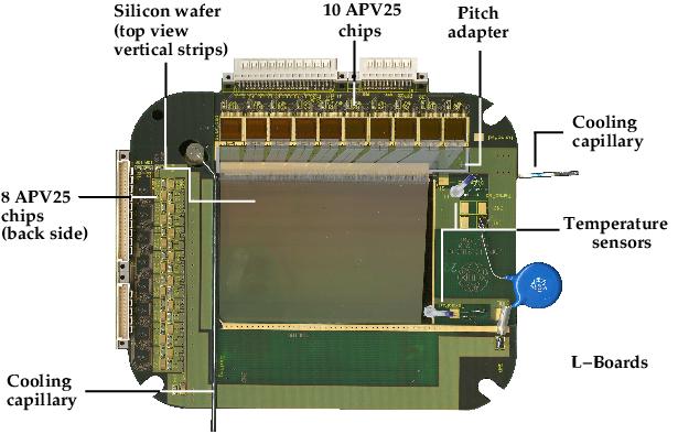
Figure 10: Front view of a COMPASS silicon detector.

The analogue signals induced on the microstrips are read out using the APV25 front-end chip, a 128-channel preamplifier/shaper ASIC with analogue pipeline, originally developed for the CMS silicon microstrip tracker [35]. Each channel of the APV25 consists of an inverter stage with unit amplification to allow signals of both polarity to be processed, and a CR-RC type shaping amplifier with a time constant of $50\,\ns$. The amplifier output amplitudes are sampled at a frequency of $38.88\,\MHz$, using the reference clock of the trigger control system (TCS) of the experiment, and stored in a 192 cell analogue pipeline. Upon arrival of an external trigger at the chip, the cells corresponding to the known trigger latency (up to $4\,\mus$) are flagged for readout. The analogue levels of the flagged cells for 128 channels are then multiplexed at $20\,\MHz$ onto a single differential output. In order to obtain time information from the signal shape, not only the sample corresponding to the peak of an in-time signal is transferred, but in addition two samples on the rising edge of such a signal are read out. While the sampling in the APV25 as well as the trigger signal are synchronised to the reference clock of the TCS, the passage of a particle is not. The resulting shift between the TCS clock phase and the actual time of particle passage, being randomly distributed in the $25.7\,\ns$ window for each event, is corrected during the reconstruction. It is determined by the difference of the rising edge of the TCS clock and the trigger time, and is measured via a TDC event by event. The multiplexed analogue data stream from each APV25 chip is digitised by a $10$ bit flash ADC, described in Sec. 8.3.1.

Two detectors make up one silicon station. They are mounted back-to-back on a fibre-glass frame such that one detector measures the horizontal ($X$) and vertical ($Y$) coordinates of a particle trajectory, while the other is rotated around the beam axis by 5^∘, providing two additional projections ($U$, $V$). [36]. The wafers are oriented such that the $X$ and $U$ planes constitute the n-side, and the $Y$ and $V$ planes the p-side of the wafer, respectively.

The residuals were calculated for standard muon run conditions using silicon detectors only, so that the track error ($<3\,\mum$) could be easily deconvoluted. The spatial resolution strongly depends on the cluster size (number of neighbouring hit strips combined to one cluster) since for more than one hit strip the spatial information can be refined by calculating the mean of strip coordinates of one cluster, weighted by the corresponding amplitude and taking into account the strip response function. The ratio of hits with cluster size 2 to hits with cluster size 1 is 1.0 for the p-side ($Y$-, $V$-planes) and 0.4 for the n-side ($X$-, $U$-planes), and is mainly given by the design of the wafer. The charge sharing is improved on the p-side by additional capacitive coupling due to intermediate strips. This results in an improved spatial resolution for the $Y$- and $V$-planes compared to the $X$- and $U$-planes, as can be seen from the residual distributions shown in Fig. 11 for a $Y$-plane, and Fig. 12 for an $X$-plane, respectively. The average spatial resolution of the COMPASS silicon detectors is $8\,\mum$ for the p-side, and $11\,\mum$ for the n-side.

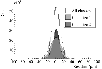
Figure 11: Residual distribution for one silicon $Y$-plane. In light grey the distribution for cluster size 1 and in dark grey for cluster size 2 are shown.

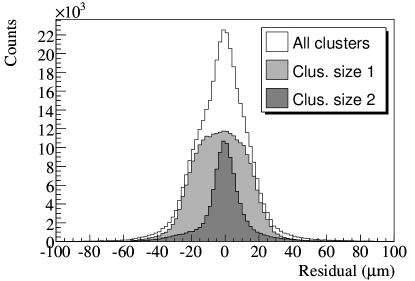
Figure 12: Residual distribution for one silicon $X$-plane. In light grey the distribution for cluster size 1 and in dark grey for cluster size 2 are shown.

Figure 13 shows the signal time distribution for one plane of a silicon detector. The average time resolution was found to be $\left<\sigma_{t}\right>=2.5\,\ns$.

Figure 13: Signal time distribution of a single projection of a silicon detector

For the COMPASS muon data taking period 2002 two silicon stations were used as beam telescope, while for 2003 and 2004 three silicon stations were employed for this purpose. In each muon data taking period each silicon detector was exposed to a fluence of about $\EE*{13}\,\mathrm{muons}/\cm^{2}$ in the central region. An increase of noise combined with a decrease of signal amplitude due to radiation damage was observed for the central region of the silicon detectors. These effects could be compensated by increasing the depletion voltage by about $15\,\V$ on average for each data taking period.

For the COMPASS hadron pilot run in 2004, two silicon stations were installed upstream of the target for the detection of beam tracks and three downstream of the target for vertex and track reconstruction. During this period the central regions of the detectors were irradiated by $8\EE{11}\,\mathrm{pions}/\cm^{2}$. For the future COMPASS data taking periods with high intensity hadron beams a fluence of about $\EE*{13}\,\mathrm{hadrons}/\cm^{2}$ will be reached in the central beam area, requiring advanced methods to increase the radiation hardness of silicon detectors. In COMPASS this will be achieved by exploiting the Lazarus effect [37], which results in a recovery of the charge collection efficiency (CCE) for irradiated detectors when operated at cryogenic temperatures. It has been shown experimentally, that the CCE recovery is greatest for operation temperatures around $130\,\K$. The silicon detector system used at present has already been designed for such cryogenic operation [36]. To this end the silicon detectors are housed in vacuum tight cryostats with low mass and light tight detector windows. The detectors will be cooled by flushing the capillary along the wafer edge (see Fig. 10) with liquid nitrogen instead of gaseous nitrogen. The liquid nitrogen distribution system is currently being developed.

5.2 Small area trackers

5.2.1 Micromegas detectors

COMPASS is the first high energy experiment using Micromegas (Micromesh Gaseous Structure) detectors [38, 39, 40]. Twelve detectors, with 1024 strips each, assembled in 3 stations of 4 planes each ($X$, $Y$, $U$, $V$), track particles in the $1\,\m$ long region between the polarised target solenoid and the first dipole magnet.

The Micromegas detector is based on a parallel plate electrode structure and a set of parallel microstrips for readout. The special feature of this detector is the presence of a metallic micromesh which separates the gaseous volume into two regions: a conversion gap where the ionisation takes place and the resulting primary electrons drift in a moderate field (here about $1\,\kV/\cm$ over $3.2\,\mm$), and an amplification gap where a higher field (here $50\,\kV/\cm$ over $100\,\mum$) produces an avalanche which results in a large number of electron/ion pairs (see Fig. 14).

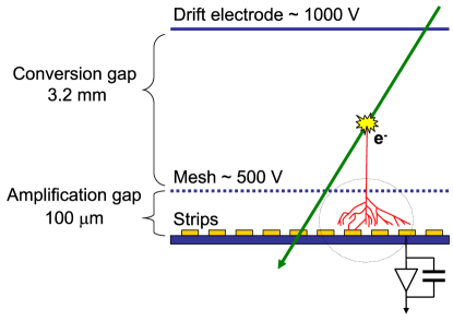
Figure 14: Principle of a Micromegas detector.

The field configuration near the mesh is such that most of the ions from the avalanche are captured by the mesh and do not drift back into the conversion gap. Consequently the ions drift over a maximum distance of $100\,\mum$ and the width of the signal induced by the ions cannot exceed the drift time over that distance, that is about $100\,\ns$. The fast evacuation of positive ions combined with the reduced transverse diffusion of the electrons and the high granularity of the detector result in a high rate capability.

The gas mixture used is Ne/C₂H₆/CF₄ (80/10/10), optimised for good time resolution. In addition, it minimises the discharge rate to $0.03$ discharges per detector and per beam spill [40].

The detector has an active area of $40\times 40\,\cm^{2}$ and a central dead zone of $5\,\cm$ in diameter. The strip pitch is $360\,\mum$ for the central part of the detector ($512\,\mathrm{strips}$), and $420\,\mum$ for the outer part ($2\times 256\,\mathrm{strips}$). In order to minimise the amount of material inside the acceptance of the spectrometer, the readout PC boards are positioned $35\,\cm$ further away by extending the readout strips outside the active area (see Fig. 15). The thickness of one detector plane in the active area is about $0.3\%$ of a radiation length.

The Micromegas are assembled in doublets of two identical detectors mounted back to back, and rotated by $90^{\circ}$ with respect to one another, so that a doublet measures two orthogonal coordinates. Fig. 15 shows a $UV$ doublet (strips at $+45^{\circ}$ in $U$-plane, and at $-45^{\circ}$ in $V$-plane).

Figure 15: A Micromegas doublet ($U$ and $V$ projections) in the COMPASS experiment. The active zone is the $40\times 40\,\cm^{2}$ internal square (1). Strips are extended (2) in order to keep the front-end electronics (3) outside the acceptance of the spectrometer.

A digital readout based on the custom-made SFE16 chip [41] is used. The chip, a 16-channel low-noise (ENC $900\,e^{-}$ at $68\,\pF$) charge preamplifier-filter-discriminator, was designed in order to stand high counting rates (up to $200\,\kHz/\mathrm{channel}$). The time window of the chip is $220\,\ns$ for typical experimental conditions. Its peaking time of $85\,\ns$ is matched to the signal rise time for a $100\,\mum$ amplification gap with the present gas mixture. The SFE16 chips are connected via LVDS links to F1-TDC chips in multi-hit mode (see Sec. 8.3.3). Both the leading and trailing edge times of the analogue signal are recorded. On the one hand, the weighted average of these two measurements yields an improved determination of the mean time by correcting for the walk. The signal amplitude, on the other hand, can be determined indirectly from the time over threshold, i.e. from the time difference of the two measurements.

In COMPASS, the Micromegas see an integrated flux of $30\,\MHz$, reaching $450\,\kHz/\cm^{2}$ close to the dead zone. The time resolution, the efficiency and the position resolution have been measured in COMPASS nominal data taking conditions of $4\EE{7}\,\mu/\mathrm{s}$ scattered on the one radiation length target, i.e. $100-200\,\kHz$ per strip, in the fringe fields of the target solenoid and the first dipole. The obtained mean time resolution is $9.3\,\ns$, as shown in Fig. 16.

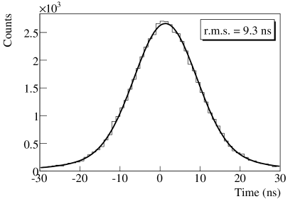
Figure 16: Distribution of the mean time measured by a Micromegas with respect to the track time for nominal intensity data. The r.m.s. width is $9.3\,\ns$.

Only signals within a time window of $\pm 50\,\ns$ are used to combine adjacent hits into clusters. The average cluster size is $2.6$ for the strips with $360\,\mum$ pitch.

The average efficiency of all Micromegas detectors was determined using charged particle tracks reconstructed in at least 20 planes of the spectrometer. It reaches $97\%$ at nominal beam intensity.

To evaluate the spatial resolution, incident tracks are reconstructed using the hits in 11 Micromegas, and the residuals in the 12th one are calculated. Fig. 17 shows the distribution of residuals for the full active area of one Micromegas detector.

Figure 17: Distribution of residuals of a Micromegas detector at high intensity. The r.m.s. width is $113\,\mum$, to which the detector contributes $92\,\mum$.

Deconvoluting the precision of the track, we obtain a spatial resolution of $90\,\mum$, averaged over all Micromegas detectors at nominal beam intensity. Their position within the spectrometer between the target solenoid and the first spectrometer dipole implies that they operate in the fringe field of both magnets, which exerts a Lorentz force on the drifting electrons. Tracks detected in the Micromegas cover angles up to $70\,\mrad$.

During the COMPASS data taking period 2002 – 2004 a total charge of $1\,\mC/\mm^{2}$ was accumulated in the sensitive region closest to the beam. The mean amplitude of the signals was continuously monitored for all detectors. No variation of amplitude (and thus of gain) was observed between the beginning and the end of the period. We conclude that no ageing has been observed and that the detector is robust and stable.

5.2.2 GEM detectors

COMPASS is the first high-luminosity particle physics experiment to employ gaseous micropattern detectors with amplification in Gas Electron Multiplier (GEM) [42] foils only. The GEM consists of a $50\,\mum$ thin Polyimide foil (APICAL^® AV [43]) with Cu cladding on both sides, into which a large number of micro-holes (about $\EE*{4}/\cm^{2}$, diameter $70\,\mum$) has been chemically etched using photolithographic techniques. Upon application of a potential difference of several $100\,\V$ across the foil, avalanche multiplication of primary electrons drifting into the holes is achieved when the foil is inserted between parallel plate electrodes of a gas-filled chamber. Suitable electric fields extract the electrons from the holes on the other side of the foil and guide them to the next amplification stage or to the readout anode. The insert in Fig. 18 depicts the electric field lines in the vicinity of a GEM hole for typical voltage settings.

As shown in Fig. 18, the COMPASS GEM detectors consist of three GEM amplification stages, stacked on top of each other, and separated by thin spacer grids of $2\,\mm$ height [44].

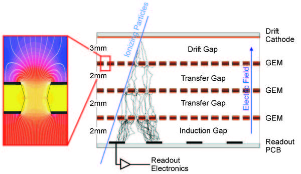
Figure 18: Schematic cross section of a triple GEM detector. The insert shows the electric field configuration for typical GEM voltages.

This scheme, developed for COMPASS together with a number of additional features as segmented GEM foils and asymmetric gain sharing between the three foils, guarantees a safe and stable operation without electrical discharges in a high-intensity particle beam [45, 46, 47], and has been adopted by various other experiments [48, 49]. The detectors are operated in an Ar/CO₂ (70/30) gas mixture, chosen for its convenient features such as large drift velocity, low diffusion, non-flammability, and non-polymerising properties.

The electron cloud emerging from the last GEM induces a fast signal on the readout anode, which is segmented in two sets of 768 strips with a pitch of $400\,\mum$ each, perpendicular to each other and separated by a thin insulating layer, as shown in Fig. 19.

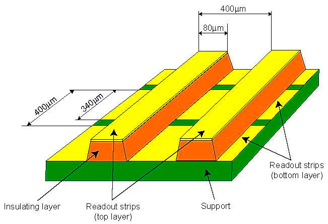
Figure 19: Schematic view of the two-dimensional readout structure of the COMPASS GEM detectors.

For each particle trajectory one detector consequently records two projections of the track with highly correlated amplitudes, a feature which significantly reduces ambiguities in multi-hit events [50].

The active area of each GEM detector is $31\times 31\,\cm^{2}$. The central region with a diameter of $5\,\cm$ is deactivated during normal high-intensity physics runs by lowering the potential difference across the last GEM foil in order to avoid too high occupancies on the central strips. At beam intensities below $2\EE{7}/\mathrm{spill}$ this area can be activated remotely to allow the detector to be aligned using beam tracks (see Sec. 10.2).

In order not to spoil the mass resolution of the spectrometer due to multiple scattering in the detector, great care has been devoted to minimise the amount of material in the active area of the detector. To this end, the gas volume is enclosed on both sides by a light-weight honeycomb structure, into which a circular hole of $5\,\cm$ diameter has been cut where the centre of the beam passes through. The material budget of one detector, corresponding to the measurement of two projections of a particle trajectory, amounts to $0.4\%$ of a radiation length in the centre, and to $0.7\%$ in the periphery.

The signals on the strips are read out using the APV25 front-end chip, in the same way as described in Sec. 5.1.2 for the silicon microstrip detectors. The readout strips are wire-bonded to the front-end PCB housing three front-end chips. Since this chip lacks proper protection against overcurrents from potential gas discharges, an external protection network consisting of a double-diode clamp (BAV99) and a $220\,\pF$ coupling capacitor was added in front of each input channel. A glass pitch adapter with aluminium strips is used to bring the strip pitch down to $44\,\mum$ to match the input pitch of the APV25.

Two GEM detectors are mounted back-to-back, forming one GEM station. One detector is rotated by $45^{\circ}$ with respect to the other, resulting in the measurement of a charged particle trajectory in four projections (labelled $XY$ and $UV$). Partial overlap with a large area tracker located at the same position along the beam guarantees complete track reconstruction and alignment.

The intrinsic properties of the triple GEM detectors have been extensively studied in test beams and in COMPASS using low-intensity beams without magnetic fields [47]. It was found that a total effective gain of $8000$ is required in order to efficiently detect minimum ionising particles in both projections.

At nominal muon beam conditions the efficiency to detect a particle trajectory in at least one of the two projections, averaged over all GEM detectors in COMPASS, was determined to be $97.2\%$ [50], with variations between different detectors on the per cent level. Apart from local inefficiencies due to the spacer grids, which account for a loss of efficiency of less than $2\%$, the distribution is found to be very uniform across each detector surface.

An offline clustering algorithm combines hits from adjacent strips to yield an improved value for the position of a particle trajectory. The average number of strips per cluster is $3.1$ for the top layer of strips, and $3.6$ for the bottom layer [47], consistent with the lateral diffusion of the charge cloud in the GEM stack. Since the GEM detectors are the most precise tracking devices in COMPASS downstream of the first dipole magnet, their spatial resolutions at standard high-intensity muon beam conditions were measured using other GEM detectors only, so that the track error could easily be deconvoluted. Figure 20 shows the distribution of residuals, i. e. the difference along one coordinate of expected track and measured cluster position, plotted for all hits on one projection of a GEM detector [50].

Figure 20: Residual distribution for one GEM projection in standard high-intensity muon beam conditions [50]. For this particular plane, the r.m.s. width of the distribution is $78.7\,\mum$, to which the detector contributes $66.4\,\mum$.

Deconvoluting the track error, the resolutions for all GEM planes in the spectrometer are found to be distributed around an average value of $70\,\mum$. This value includes a contribution of overlapping clusters due to pile-up in high intensity conditions of about $20\,\mum$. Variations for single detectors are due to the effect of the fringe field of the first spectrometer magnet, and the influence of multiple scattering in the material preceding the respective detector. For all detectors the distortion of charge clouds in the immediate vicinity of the spacer grids deteriorates the average resolution by about $4\,\mum$.

In addition to an improved spatial resolution the analogue readout method also allows to extract time information by sampling the signal at three consecutive points in time. Knowing the detector response to a minimum ionising particle, the hit time can be determined from ratios of the three measured amplitudes. With this method, an average time resolution of $12\,\ns$ was found for the GEM detectors in the high intensity muon beam [50], as can be seen from Fig. 21.

Figure 21: Distribution of cluster time measured by a single GEM plane by sampling the analogue signal at $40\,\MHz$, with respect to the track time [50].

In total, 11 GEM detector stations, i.e. 22 detectors, are installed in COMPASS. Out of these, seven were operational from 2001 on, three stations were added in 2002, and one additional station was added for the 2004 run. Depending on the position in the spectrometer, particle rates as high as $25\,\kHz/\mm^{2}$ are observed close to the central inactive area, equivalent to a total collected charge since 2002 of more than $2\,\mC/\mm^{2}$. Despite of this high-radiation environment, no degradation of performance has been observed. Laboratory tests, in which a total charge of $7\,\mC/\mm^{2}$ was collected using Cu X-rays without loss of gain [51], show that the GEM detectors will operate reliably well beyond the second phase of COMPASS, which started in 2006.

5.3 Large area trackers

5.3.1 Drift chambers

Three identical drift chambers (DC) are installed in COMPASS. Their design was optimised for operation upstream of the first dipole magnet (SM1), where the total particle flux through the chamber is higher by almost a factor of three compared to the downstream side due to the low-energy background which is bent away by the magnet. One DC is installed upstream, and two DCs downstream of the SM1 magnet. All three DCs have an active area of $180\times 127\,\cm^{2}$, fully covering the acceptance of the SMC target magnet upstream as well as downstream of SM1.

Each DC consists of eight layers of wires with four different inclinations: vertical ($X$), horizontal ($Y$) and tilted by $20^{\circ}$($U$) and $-20^{\circ}$($V$) with respect to the vertical direction. The tilt angle and the ordering of planes ($XYUV$ along the beam) was chosen in order to minimise the number of fake tracks during the reconstruction.

Each layer of wires consists of 176 sensitive wires of $20\,\mum$ diameter, alternated with a total of 177 potential wires with $100\,\mum$ diameter, and is enclosed by two Mylar^® [52] cathode foils of $25\,\mum$ thickness, coated with about $10\,\mum$ of graphite, defining a gas gap of $8\,\mm$ extent. Two consecutive layers of the same inclination are staggered by $3.5\,\mm$ (half a drift cell) in order to solve left-right ambiguities. During operation of the chamber the cathode foils, the sensitive wires and the potential wires are kept at around $-1700\,\V$, $0\,\V$ and $-1700\,\V$, respectively. The total material budget of each detector (8 layers) along the beam path, including the gas mixture, is $0.32\%$ of a radiation length.

Drift cell boundaries (Fig. 22) are defined by the cathode foils, normal to the beam direction, and by two potential wires separated by $7\,\mm$.

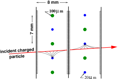
Figure 22: Drift cell geometry of the COMPASS drift chambers.

The choice of a small drift cell size ($8\times 7\,\mm^{2}$) was triggered by counting rate considerations. Smaller drift cells decrease the incident flux per cell and reduce the electron drift time. The reduced drift time has an additional advantage: it allows the use of a shorter time window and consequently minimises the number of uncorrelated particles.

Fig. 23 shows that the hit rate per wire at a distance of $15\,\cm$ from the beam reaches $800\,\kHz/\mathrm{wire}$ upstream of SM1. Downstream of SM1, the maximum hit rate per wire is reduced to $300\,\kHz$.

Figure 23: Hit rate versus wire number for one DC wire layer upstream of SM1 at nominal beam intensity with the central zone deactivated.

In order to avoid even higher rates near the beam a central dead zone of $30\,\cm$ diameter was implemented for all layers. As a segmented part of the whole cathode foil, this dead zone has an independent high voltage supply. During standard data taking the central zone is deactivated by keeping the high voltage (HV) supply at low enough voltage, so that the local efficiency vanishes. For alignment purposes at low beam intensity, the dead zone is activated by setting the HV to the nominal value of the potential wires ($-1700\,\V$).

The gas mixture was chosen in order to fulfil several constraints. First it should ensure good spatial resolution. Second it should feature a nearly linear time-vs-distance dependence (RT relation). Third it has to be fast enough so that the occupancy time is minimised. Finally it should provide good efficiency and a large HV plateau. The best compromise was obtained by a mixture of Ar/C₂H₆/CF₄ (45/45/10). The Argon component ensures high primary electron rate (about $100$ per MIP), the C₂H₆ component serves as a quencher and the CF₄ is used to increase the drift velocity, to $77\,\mm/\ns$ ($13\,\ns/\mm$). With this mixture the gain was measured to be $2\EE{4}$ for a HV of $1800\,\V$, while full efficiency is obtained at a voltage slightly below $1600\,\V$. In order to limit cathode currents below $15\,\muA$, DC1 was operated at $1650\,\V$, DC2/3 at $1750\,\V$.

The detector output signals are read by the ASD8-B chip [53], an eight-channel preamplifier / amplifier / discriminator with $3\,\ns$ rise time. Eight ASD8 chips are mounted on a single analogue board of 64 channels. A discriminator threshold of about $25000\,\mathrm{e}^{-}$ is set to each pair of wire layers (352 wires); it can be independently adjusted on each ASD8 chip. The discriminated signals are sent to the F1-TDC digitisation board. The 64-channel F1-TDC board used for the drift chambers is identical to the one used for the Micromegas detectors (see Sec. 5.2.1).

Particular care was taken in minimising the electronic noise of the whole system. In both analogue and digital boards the signal wire layers are enclosed in between two grounded copper planes. Multiple connections are made between the board ground and the detector structure; this common ground is also shared with the low-voltage power supplies. As a result the measured noise figure at nominal threshold is in the range $10-100\,\Hz/\mathrm{channel}$.

The performances of the DCs were studied at several beam conditions, the incident flux being roughly proportional to the beam intensity. Figure 24 shows the RT relation for one layer of a DC, measured in a low intensity beam.

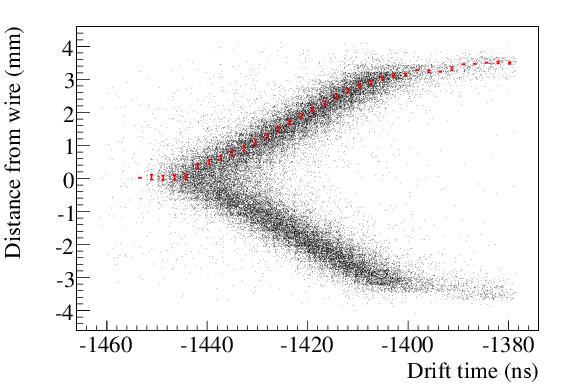
Figure 24: Measured RT relation for one layer of a DC.

At nominal COMPASS beam conditions the mean layer efficiency is $95\%$ or higher, the efficiency being higher for the DC detectors located downstream of SM1. Nearly all inefficiency is due to pile-up at high rates.

The spatial resolution of the DC detectors was evaluated using the residuals of the fitted tracks for each wire layer. Combining the residuals from two wire layers with the same orientation allows us to separate the intrinsic layer resolution from the uncertainty due to the track fitting. At nominal muon beam intensity a mean value for the resolution of a single DC wire layer of $270\,\mum$ was measured, averaged over all layers and over the full active surface, with maximum deviations from this value of $\pm 20\,\mum$ (see Fig. 25).

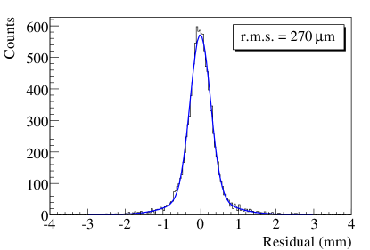
Figure 25: Single DC layer residual distribution in the high intensity beam (here: DC1 $X$).

Compared to the expected intrinsic resolution, this value includes a deterioration due to two effects: (i) the large halo coming along with the high intensity beam, which contributes about $30\,\mum$, and (ii) the large fringe field of the SM1 magnet present in all DCs, which exerts a Lorentz force on the drifting electrons, and contributes about $20\,\mum$ for the $X$, $U$ and $V$ layers. For the $Y$ layers the electrons drift mainly parallel to the magnetic field, limiting the Lorentz effect to a few $\mum$ only. The resulting resolution of one DC (8 wire layers) for the horizontal coordinate (bending direction of the dipole) is $110\,\mum$, while it is $170\,\mum$ for the vertical coordinate.

5.3.2 Straw tube chambers

Straw tube drift chambers [54] are used for the tracking of charged particles produced at large scattering angles ($15-200\,\mrad$) in the Large Area Tracking section (LAT) of COMPASS downstream of the first spectrometer magnet (SM1).

The straw tubes are made of two layers of thin plastic films. The inner layer consists of a carbon loaded Kapton^® 160 XC 370 [52] foil with a thickness of $40\,\mum$. It is glued onto the second layer, an aluminised Kapton^® foil of $12\,\mum$ thickness. The anode wires are made of gold-plated tungsten with $30\,\mum$ diameter. They are centred in the straw tubes by two end-plugs and four small plastic spacers, which are positioned at intervals of about $60\,\cm$ along each tube. The counting gas is supplied through the end-plugs and a gas-manifold, which is integrated into the aluminium frame construction.

In total 12440 straw tubes are assembled into 15 detectors. To resolve left-right ambiguities of a particle trajectory, each detector consists of two staggered layers of straws, which are glued together and mounted onto an aluminium frame for mechanical stability. Each detector has an active area of about $9\,\m^{2}$ and is divided into three sections. Fig. 26 shows a schematic view of a detector (type X).

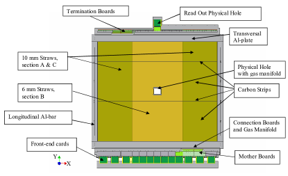
Figure 26: Schematic view of a COMPASS straw detector (type X) [54].

The central part (section B, see Fig. 26), being closer to the beam axis, is exposed to higher rates. This part is made of 190 long and 64 short straws per layer, all with an outer diameter of $6.14\,\mm$, forming a central dead zone of about $20\times 20\,\cm^{2}$. It has a rectangular hole without material of about $20\times 10\,\cm^{2}$ for the beam. The outer two parts (section A and C) each have 96 straws with $9.65\,\mm$ outer diameter. The chosen diameters are a compromise between minimising the number of channels and production cost, and keeping the occupancy in each tube below $2\%$ at maximum beam rates. As a fast counting gas a mixture of Ar/CO₂/CF₄ (74/6/20) is used. The straw tubes are operated at a high voltage of $1950\,\V$, corresponding to a gain of $6\EE{4}$.

In order to measure three projections of a particle trajectory, one station consists of three detectors, one with vertical, one with horizontal and one with inclined straw tubes. The detectors with inclined straws are rotated by $10^{\circ}$ with respect to the vertical ones. The detectors with vertical and inclined straws are of the same type (called type X), while the ones with horizontal straws have a slightly different geometry (type Y). The exact dimensions of both types are given in table 7.

Table 7: Geometrical properties of $X$ and $Y$ types of straw detectors.

Type	Sensitive area $X\times Y$ ($\mm^{2}$)	Length of straws ($\mm$)	Number of straws with outer diameter of		Number of readout channels	Overall dimensions $X\times Y$ ($\mm^{2}$)
			$6.14\,\mm$	$9.65\,\mm$
		3202	380	384
X	$3232\times 2802$	1523	128		892	$3570\times 4117$
		3652	320	256
Y	$3254\times 2427$	1752	128		704	$4567\times 3160$

The thickness of one detector along the beam direction is $40\,\mm$. The amount of material in the active part of the detector was minimised with respect to scattering and secondary interactions, and corresponds to $0.2\%$ of a radiation length for one detector, not taking into account the detector gas.

The length of a COMPASS straw tube increases with increasing humidity. The relative elongation was measured to be about $3\EE{-5}$ for a humidity change of $1\%$ [54], resulting in increased tension on the frame or, even worse, in a bending of straws. In order to keep the humidity constant, each straw station is surrounded by a protective gas volume of N₂ gas, enclosed by $12\,\mum$ thin Mylar^® [52] foils which are aluminised on both sides.

The mechanical precision of wires averaged over all detectors was determined to be $170\,\mum$ (r.m.s.) by measuring the coordinates of the wires at all spacer and end-plug positions with a triple stereo imaging X-ray scanner [55]. The deviation of the wire with respect to its nominal position is then used in the offline data analysis as a correction to the measured coordinate, reducing the uncertainty of the mechanical wire position to $60\,\mum$.

The electrical connections to the anode wires are fed through the gas tight volume by connecting boards. The straws are read out on the bottom side only, while they are terminated on the top side by termination boards. The signals of the straws are amplified and discriminated by the ASD8-B chip, already described in Sec. 5.3.1, and digitised by the F1-TDC chip, described in Sec. 8.3.3. The discriminator thresholds are typically set to $6\,\fC$, resulting in a noise level of $5\,\kHz/\mathrm{channel}$. Eight ASD8 and F1-TDC chips, corresponding to sixty-four channels, are assembled on one front-end card. Each front-end card is plugged to a motherboard, which also contains the high voltage distribution circuit and a test pulse line for calibration. Motherboards and front-end cards are supported by the chamber frame.

The performance of the straw tube chambers has been evaluated in both COMPASS low and high intensity beams. At nominal muon beam intensity tracks reconstructed by the COMPASS offline analysis software (CORAL, see Sec. 10.1) were used to determine, for each wire separately, the relation between the measured drift times and the distances of tracks to the anode wire. Figure 27 shows this RT relation for one single $6\,\mm$ straw tube.

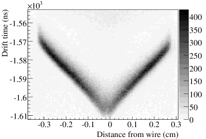
Figure 27: RT relation for a single $6\,\mm$ straw tube for particle tracks measured with the $160\,\GeV/c$ muon beam [54].

Once this relation has been established, the resolution of a given straw tube can be determined from the r.m.s. width of the distribution of track residuals, taking into account the corrections from the X-ray scan of wire positions. Fig. 28 shows the r.m.s. widths of single-channel residual distributions versus channel number for the central part ($6\,\mm$ tubes) of one straw tube layer, where the number of good tracks from other detectors is still sufficiently high.

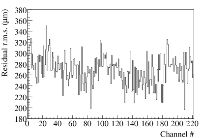
Figure 28: R.m.s. widths of single-channel residual distributions versus channels number for all $6\,\mm$ straw tubes of one layer.

Averaging over several layers of $6\,\mm$ straws, a mean value for the resolution of $270\,\mum$ for one straw layer under nominal COMPASS muon beam conditions is obtained. For one straw detector (two layers), the average resolution is then $190\,\mum$. Intrinsic resolutions without the effects of temperature variations and of the overall tracking are given in Ref. [54]. Dedicated beam tests already showed earlier that resolutions are the same for $6\,\mm$ and $10\,\mm$ straws [54]. In these tests it was also shown that the mean efficiency of a straw detector, i.e. the probability for either of the two layers to detect a hit, is higher than $99\%$, with the inefficiencies being concentrated along the mechanical edges of the detector.

5.3.3 Multiwire proportional chambers

The tracking of particles at large radial distances to the beam in the SAS is mainly based on a system of multiwire proportional chambers (MWPC). A total of 34 wire layers, corresponding to about $25000$ detector channels, is installed and operated since the year 2001. All layers are characterised by a wire length of about $1\,\m$, a wire diameter of $20\,\mum$, a wire pitch of $2\,\mm$ and an anode/cathode gap of $8\,\mm$.

In COMPASS three different types of MWPC are used, named type-A, type-A^⋆ and type-B. Type-A detectors have three anode wire layers, one vertical ($X$) and two tilted by $\pm 10.14^{\circ}$ with respect to the vertical axis ($U$, $V$), and an active area of $178\times 120\,\cm^{2}$. Type-A^⋆ detectors are similar to type-A, with an additional horizontal wire layer ($Y$). Type-B detectors have a smaller active area ($178\times 80\,\cm^{2}$) and only two wire layers, one vertical ($X$) and one tilted by $10.14^{\circ}$ ($U$ or $V$). Type-B stations are composed of two detectors with inclined wire layers with opposite orientations, fixed together; only three layers, one vertical and two tilted, are read out. All wire layers are enclosed from both sides by $10\,\mum$ thick graphite coated Mylar^® [52] cathode foils, to provide field symmetry and to enclose the detector gas. A central dead zone of $16-22\,\mm$ diameter, depending on the location of the chamber along the beam axis, was realized by removing the graphite coating from the foils. The total thickness corresponds to $0.2\%$, $0.3\%$, and $0.2\%$ of a radiation length for A-, A^⋆-, and B-type chambers, respectively. The detector characteristics are summarised in Table 8.

Table 8: Characteristics of the COMPASS MWPC detectors.

	A-type	A∗-type	B-type
# of chambers	7	1	6
Active area	$178\times 120\,\cm^{2}$	$178\times 120\,\cm^{2}$	$178\times 80\,\cm^{2}$
# of layers/chamber	3	4	2
Planes	$X$, $U$, $V$	$X$, $U$, $V$, $Y$	$X$, $U/V$
Dead zone $\oslash$	$16-20\,\mm$	$16\,\mm$	$22\,\mm$
Wire pitch	$2\,\mm$	$2\,\mm$	$2\,\mm$
Anode/cathode gap	$8\,\mm$	$8\,\mm$	$8\,\mm$
# of wires/plane	752 ($X$, $U$, $V$), 512 ($Y$)	752 ($X$, $U$, $V$), 512 ($Y$)	752 ($X$, $U$, $V$), 512 ($Y$)

The MWPC are operated with a gas mixture of Ar/CO₂/CF₄ in proportions 74/6/20. The addition of a fast gas as CF₄ is a crucial requirement to operate MWPC detectors in high rate environments, without introducing excessive detector dead time. The typical time jitter of the wire signal with the chosen gas mixture is about $80\,\ns$, compatible with the typical electron drift velocity in the gas mixture used. At nominal high voltage of $4250\,\V$ the gain is between $3.5\EE{4}$ and $4\EE{4}$.

The read-out electronics is distributed on two printed circuit boards: the mother board, fixed to the chamber frame, and the front-end board, where the signals of the chamber are discriminated and digitised. The data is transferred through a fast serial link to the CATCH modules. Figure 61 (see Sec. 8.4.1) shows the functional block diagram of the read-out electronics.

The front-end electronic is organised in triplets of cards that can read 64 channels per board. Each card houses the MAD4 preamplifier/discriminator chips [56] with a peaking time of $5\,\ns$, the F1-TDC chips (see Sec. 8.3.3), and the threshold DACs. The three cards are connected together by a fast LVDS bus, which distributes the reference clock, trigger and synchronisation signals. Production cost has been reduced by housing both analogue and digital parts on the same PCB. Moreover central and side boards share a common design, except for the bus controller and the parallel-to-serial converter chips for fast data transmission to the CATCH module (see Sec. 8.4), which are housed only on the central board. For noise prevention all the voltages required by the card components are regulated on–board, and separate grounds for analogue and digital parts are used. A test system has been developed, capable of injecting a charge pulse similar to the signal of a minimum ionising particle crossing the chamber into each wire. The system is composed of a VME control board and pulser boxes fixed to the frame of each MWPC detector. It allows tests and calibration of the front-end cards and of the read-out system, including the input connectors.

In a typical MWPC an ionising particle traversing the detector may induce a signal on several neighbouring wires. The position of a hit can then be calculated from the weighted mean of coordinates of adjacent wires with signals (clusters). For the COMPASS MWPC, the cluster size distribution has an approximately exponentially decreasing shape with a probability of about $30\%$ for a cluster size larger than unity. The spatial resolution of each single MWPC layer was measured in a standard high-intensity muon beam using a sub-sample of tracks reconstructed in the GEM stations coupled to the MWPCs. The MWPC layers have been excluded from the tracking. The residual distribution has an r.m.s. width of $1.6\,\mm$ (see Fig. 29).

Figure 29: Typical MWPC residual distribution for standard physics conditions, showing the difference between wire cluster position and extrapolated track position along the axis perpendicular to the wire layer.

The beneficial effect of wire clusterisation on the measured spatial resolution is evident from a separate analysis of clusters with different sizes, as shown in Fig. 30 for cluster size one and two.

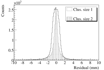
Figure 30: Residual distributions of an MWPC layer for cluster sizes 1 (transparent) and 2 (grey).

The MWPC detectors have been operated in stable conditions at nominal high voltage since the year 2001. Fig. 31 shows the average efficiencies of all MWPC stations during the 2004 data taking period.

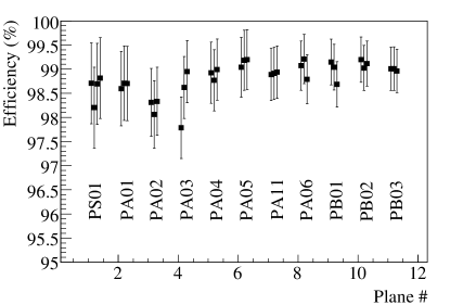
Figure 31: Efficiencies of all MWPC stations during the 2004 data taking period. The average efficiency is $>98\%$.

5.3.4 Large area drift chambers

To provide tracking for charged particles deflected by a large angle in the COMPASS SAS a system of six large area drift chambers is used. A detailed description of the prototype chamber can be found in [57]. The basic detector characteristics are summarised in Table 9.

Table 9: Basic characteristics of the COMPASS large area drift chambers.

	$XY$-type	$XV$-type	$XU$-type	$YV$-type	$YU$-type
# of chambers	2	1	1	1	1
Active area	$500\times 250\,\cm^{2}$	$500\times 250\,\cm^{2}$	$500\times 250\,\cm^{2}$	$500\times 250\,\cm^{2}$	$500\times 250\,\cm^{2}$
# of layers/chamber	4	4	4	4	4
Planes	$X$, $Y$	$X$, $V$	$X$, $U$	$Y$, $V$	$Y$, $U$
Dead zone $\oslash$	$500\,\mm$	$1000\,\mm$	$1000\,\mm$	$1000\,\mm$	$1000\,\mm$
Anode wire pitch	$4\,\cm$	$4\,\cm$	$4\,\cm$	$4\,\cm$	$4\,\cm$
Anode/cathode gap	$10\,\mm$	$10\,\mm$	$10\,\mm$	$10\,\mm$	$10\,\mm$
# of wires/plane	260 ($X$), 130 ($Y$)	260 ($X$), 288 ($V$)	260 ($X$), 288 ($U$)	130 ($Y$), 288 ($V$)	130 ($Y$), 288 ($U$)

Each chamber has an active area of $5\times 2.5\,\m^{2}$, and consists of 4 sensitive anode wire layers with a wire pitch of $4\,\cm$, separated by layers of cathode wires with a pitch of $2\,\mm$. The total number of readout channels is $2750$. All chambers have two planes, each plane consisting of two wire layers. Four of the chambers have $X$ layers, coupled with $Y$ ($XY$-type), $V$ ($+30^{\circ}$ with respect to the $X$ layer, $XV$-type), or $U$ ($-30^{\circ}$, $XU$-type) layers. The two other chambers are of $YV$-type and $YU$-type. The two wire layers with the same orientation within one chamber are shifted by half the wire pitch.

The diameter of the anode wire is $20\,\mum$, while the cathode is made of $100\,\mum$ wires. The anode/cathode gap is $10\,\mm$. The cathode wires are inclined by $5^{\circ}$ with respect to vertical direction to provide better field homogeneity. The signal wires are separated with field wires of $200\,\mum$ diameter.

To guarantee a reliable operation in a high particle rate environment, a dead region with a diameter of $0.5\,\m$ and of $1\,\m$ was implemented in the centre of each layer of $XY$-type, and of $XV$, $XU$, $YV$ and $YU$-type chambers, respectively. To this end a galvanisation technique was developed in order to enlarge the radius of the sense wires up to $100\,\mum$, thus preventing gas amplification in this region (see Fig. 32).

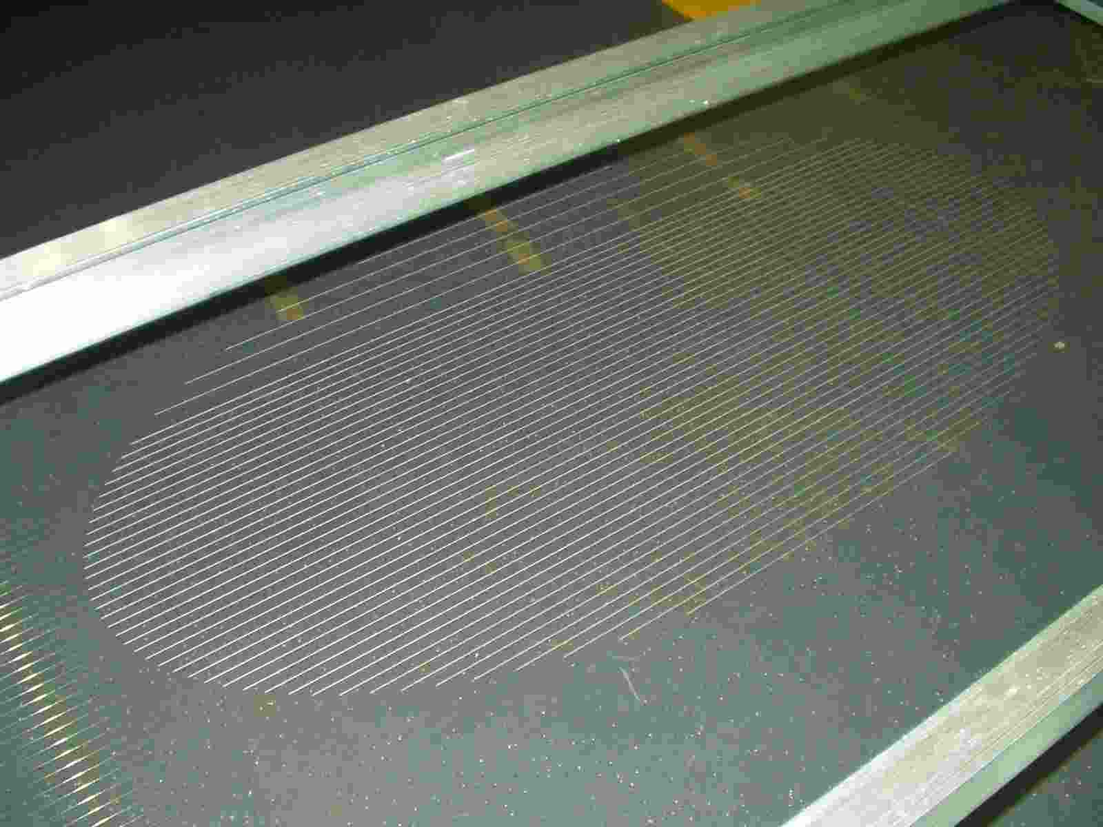
Figure 32: The dead region of a large area drift chamber. In the central part of the chamber (diameter 1 meter) the sensitive wire thickness is 5 times larger than in the active part of the chamber.

A fast CF₄-based gas mixture, Ar/CF₄/CO₂ (85/10/5), is used to increase the drift velocity, which is important for efficient track reconstruction. The signal wires are operated at a high voltage of $1925\,\V$, the field wire potential is kept at $-800\,\V$.

Similarly to the MWPCs (see Sec. 5.3.3), the readout electronics is based on MAD4 amplifiers/discriminators and F1-TDC chips. A threshold value of $5\,\fC$ is used.

The average layer efficiency was measured to be $93\%$. The gas mixture and high voltage values were optimised in order to homogenise the drift velocity in the drift gap. The resulting RT relation plot of one large area drift chamber is shown in Fig.  33.

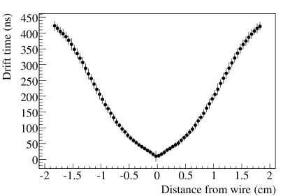
Figure 33: RT relation for one large area drift chamber.

A mean spatial resolution of $0.5\,\mm$ was achieved in the 2004 run.

6 Particle identification

The COMPASS Large Angle and Small Angle Spectrometers (LAS and SAS) include several particle identification detectors. A RICH counter located in the first spectrometer (RICH-1, see Sec. 6.1) separates outgoing hadrons into pions, kaons and protons, up to momenta as large as $43\,\GeV/c$. Two hadron calorimeters (HCAL1 and HCAL2, see Sec. 6.3.1 and 6.3.2) measure the energy of hadrons and provide a complementary trigger signal. An electromagnetic calorimeter (ECAL2, see Sec. 6.3.3) determines the energies of the photons and electrons emitted at small angles. Finally, in both LAS and SAS, scattered muons are detected in two muon wall systems (MW1 and MW2, see Sec. 6.2.1 and 6.2.2) both consisting of medium resolution tracking detectors combined with a hadron absorber.

6.1 RICH-1 detector

The COMPASS RICH-1 [58] is a large-size Ring Imaging Cherenkov detector which performs hadron identification in the domain between $5\,\GeV/c$ and $43\,\GeV/c$. It has large transverse dimensions (it covers the whole angular acceptance of the COMPASS LAS, i.e. $\pm 250\,\mrad$ in the horizontal plane and $\pm 180\,\mrad$ in the vertical plane), high-rate capability and introduces minimum material in the region of the spectrometer acceptance. Its large-volume vessel (see Fig. 34) is filled with C₄F₁₀ radiator gas. Cherenkov photons emitted in the gas are reflected by two spherical mirror surfaces. The photons are converted to electrons by the CsI photocathodes of eight MWPCs, which amplify the single photoelectrons and detect them.

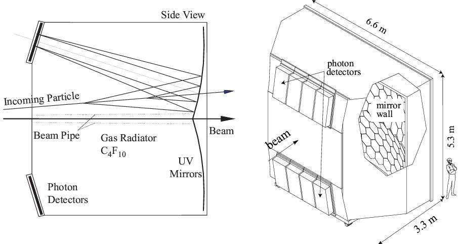
Figure 34: COMPASS RICH-1: principle and artistic view.

Hadron identification in the multi-$10\,\GeV/c$ momentum domain imposes C₄F₁₀ as a radiator gas, thanks to its low chromaticity, in spite of its high refractive index. The quest for sufficient number of Cherenkov photons for this gas determines the overall length of the radiator vessel (see Fig. 34) to be of about $3\,\m$. Requirements for low background, minimum material in the spectrometer acceptance and the need to operate the MWPC-CsI detectors in an environment of a reduced particle flux, dictate the final RICH-1 geometry: the photon detectors are placed far from the beam line and outside the spectrometer acceptance. The corresponding mirror system consists of two reflecting surfaces located off beam axis, such that the Cherenkov ring images are focused outside the LAS acceptance.

The RICH-1 geometry results in a photon detector surface of $5.6\,\m^{2}$. The surface is covered with eight proportional chambers (MWPCs), equipped with CsI photon converter layers. CsI photon converters have good quantum efficiency for wavelengths below $200\,\nm$ only; this property implies compatibility in the very UV (VUV) domain of both the mirror system and the gas radiator. Quartz windows separate the radiator gas from the photon detector; the quartz optical properties impose the lower limit of the useful wavelength at $\approx 165\,\nm$. A dedicated radiator gas system establishes continuous gas circulation in a closed loop and ensures both optimum VUV transparency and constant relative pressure in the vessel.

6.1.1 RICH-1 gas and gas system

The RICH-1 gas radiator vessel has a length of $3\,\m$ and a volume of about $80\,\m^{3}$. The refractive index of the C₄F₁₀ gas ($n-1=0.0015$ for $7\,\eV$ photons) and its low chromaticity ($\mathrm{d}\!\!\;n/\mathrm{d}\!\!\;E\sim 5\EE{-5}\,\eV^{-1}$ at $7\,\eV$) make it adequate for hadron identification above $10\,\GeV/c$. The gas is handled by a dedicated gas system [59], which controls the pressure inside the vessel, keeps the radiator gas transparent in the VUV domain, fills the vessel with the radiator gas and recovers it in the storage tank.

The gas in the vessel must be kept in well controlled relative pressure conditions in order to avoid damages to the two thin vessel walls in the acceptance region, and to avoid mechanical deformation of the vessel itself, which can be transfered to the mirror wall. The vessel pressure is kept constant within $1\,\Pa$ over months of operation, while the maximum allowed variations are an order of magnitude larger.

The radiator transparency in the light wavelength region between 160 and $200\,\nm$ is essential for RICH-1 operation, as it influences directly the number of photons observed per ring. The commercially available C₄F₁₀ material is fully opaque in the VUV domain, as it contains VUV absorbing impurities [60]; a cleaning procedure is then mandatory before the insertion of the gas in the RICH vessel. Cleaning has been performed in liquid phase up to year 2001 and in gas phase later, with typical material losses related to the cleaning procedure of around 20%. The gas is also constantly filtered from water vapour and oxygen contaminations during operation. This is done by continuously circulating the gas in a closed loop circuit through a Cu catalyst at $\approx 40^{\circ}$C to remove oxygen and through a 5A molecular sieve at $\approx 15^{\circ}$C to trap the water vapour traces. As a result, water vapour traces below 1 ppm and O₂ below 3 ppm are routinely obtained.

The VUV light transmission is measured online using two complementary systems. A dedicated setup performs an integral measurement over the range from $160\,\nm$ to $210\,\nm$ using a UV lamp and a solar-blind photomultiplier. A system based on the use of an UV lamp and a monochromator measures the transmission as a function of the light wavelength in the VUV range of interest. Good transparency of the gas radiator, stable over months, was achieved from 2003. Figure 35 shows a typical transmission curve in the VUV domain, with the main contributions to the VUV light absorption: Rayleigh scattering, O₂ and H₂O.

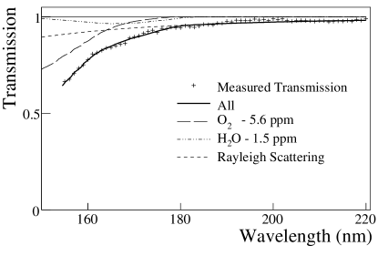
Figure 35: Typical UV light transmission through 1.87 m of C₄F₁₀, as measured online during data taking (crosses). The solid curve is a fit to the data. The main contributions to the UV light absorption are also shown.

6.1.2 RICH-1 mirror system

The RICH-1 optical system [61] consists of two VUV reflecting spherical surfaces of total area larger than $21\,\m^{2}$ and a radius of curvature of $6600\,\mm$. It was designed to focus the images outside the spectrometer acceptance on the photon detectors. The surface of the plane photon detectors is a rough approximation of the spherical focal surface. The two mirror surfaces are a mosaic type composition of 116 spherical mirror units: 68 of them are regular hexagons with a side length of $261\,\mm$, the other 48 are pentagons with six different sizes. The clearance left between adjacent mirrors results in a 4% loss of reflecting surface. This optical arrangement, coupled to the $3\,\m$ long radiator, results in a geometrical aberration of $0.32\,\mrad$ for images produced by particles incident at angles of a few $\mrad$, and increasing for particles incident at larger angles.

The mirror substrate is a borosilicate glass, $7\,\mm$ thick, corresponding to about 5.5% of a radiation length. All individual substrate pieces have been characterised by measuring the radius of curvature and the diameter of the image of a point-like source. The roughness of the polished surfaces has been measured by sampling. Good reflectance in the VUV region is obtained by applying a reflective layer (Al, $80\,\nm$) covered by a protective layer (MgF₂, $30\,\nm$ ). The reflectance, as measured shortly after the production in the useful wavelength interval ($165-200\,\nm$), was found to be in the range $83-87$%. The measurements were repeated after 1 and 2 years of operation. Except a short term degradation at small wavelengths, stable reflectance values above $165\,\nm$ (see Fig. 36) have been observed.

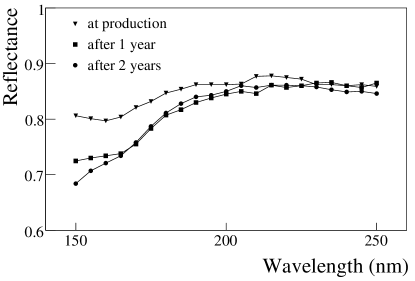
Figure 36: Measured reflectance for a typical mirror piece. The measurements have been performed shortly after production, 1 year and 2 years later.

The mechanical structure supporting the mirror wall has a net-like configuration designed to minimise the amount of material in the spectrometer acceptance; the mirrors are suspended to the nodal points, which lay on a sphere; as a consequence, only angular adjustment of the mirror units is needed. Each mirror is equipped with a joint which allows it to rotate around two orthogonal axes with angular resolution better than $0.1\,\mrad$. The overall amount of material used for the mechanical supports is equivalent to 2.5% of a radiation length.

Alignment of the RICH-1 mirrors is performed inside the vessel. Since the loci of the spherical surfaces lay outside the vessel volume, an original alignment procedure was adopted. The coordinates of the two sphere centres are known in the vessel reference frame. The coordinates of a theodolite are measured in the same frame. The theodolite axis is oriented along the straight line joining its centre and the centre of the sphere (reference line). If the mirror which is just in front of the theodolite is perfectly aligned, the normal to the mirror surface at the intersection point with the reference line will also lie along this line. In the alignment procedure, the mirror is rotated until the two lines coincide. The accepted residual misalignment angle is $<0.1\,\mrad$ corresponding to the precision with which the reference line is defined.

6.1.3 RICH-1 photon detectors

The photon sensitive surface area of RICH-1 is equipped with eight large-size MWPCs ($576\times 1152\,\mm^{2}$) CsI photocathodes [62]: this is the largest photon detection system of this kind in operation so far. The main parameters of the MWPCs are those optimised during the RD26 collaboration studies [63, 64, 65]: $20\,\mum$ diameter wires, $4\,\mm$ wire pitch, $2\,\mm$ anode-cathode gap and a photocathode surface segmented in $8\times 8\,\mm^{2}$ pads. The eight photon detectors have 82944 pad channels in total. A quartz window separates the detector from the vessel. The MWPC chambers are filled with pure methane, as it is transparent to photons in the useful energy range. The overall detector structure is illustrated in Fig. 37.

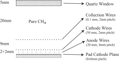
Figure 37: Cross section of the RICH-1 photon detector.

The CsI coating of the photocathodes has been performed at CERN following a procedure established by the RD26 collaboration and later optimised for ALICE HMPID [66] and COMPASS applications. Severe constrains have been imposed on the tolerances of the MWPC mechanical parameters: the required precision on anode-cathode gap is $50\,\mum$ , the anode wire mechanical tension is within 5% of the nominal values.

The large photocathode elements are never exposed to air after coating with the CsI layer, as impurities and, in particular, water vapour can degrade the quantum efficiency. The possible contamination is monitored by measuring the oxygen level of the atmosphere to which the photocathodes are exposed. For this goal, the photocathode units are always handled in dedicated glove boxes. A dedicated photocathode transportation system has been designed and built; it allows the transportation of up to four photocathodes, each protected with a gas-tight cover and under a continuous flux of nitrogen filtered in a closed loop.

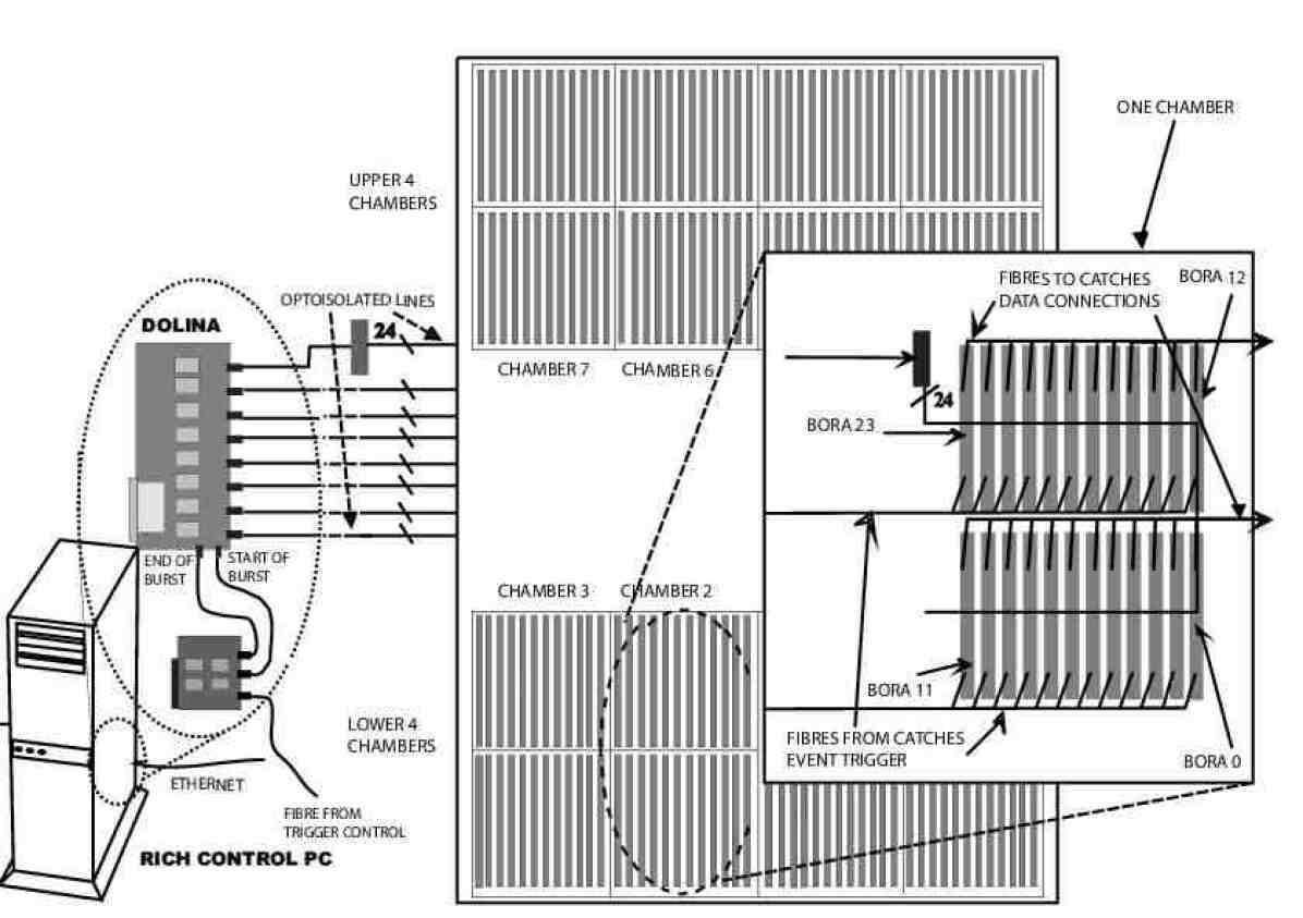
Figure 38: The figure shows a top-level view of the front-end data acquisition of RICH-1. Each of the 192 BORA boards is directly connected through a fibre optical link to the COMPASS DAQ system for data transfer and through a slower network to the controlling PC computer.

MWPCs with CsI photocathodes must be operated at moderate gain due to the presence of the photosensitive CsI layer. Because of the radioactive environment the photon detectors may occasionally exhibit electrical instabilities with long ($\sim$1 day) recovery time, clearly related to the combined effect of the level of the applied voltage and the ionising particle flux [67]. Tiny local imperfections of the detectors favour the instabilities [68]. Great care in the mechanical precision of the MWPCs as well as in the uniformity of the anode wire tension and validation in the high-flux Gamma Irradiation Facility at CERN have allowed us to obtain stable operation at gains up to $5\EE{4}$. The electrical stability of the MWPCs with CsI has been improved in time. In 2001, 25% of the MWPCs area was stable; in 2002, 75%; in 2003 and 2004, 97%.

6.1.4 RICH-1 readout system

Signals generated in MWPCs by single electrons, as it is the case for the photoelectrons due to the conversion of Cherenkov photons, have amplitude spectra described by Polya functions. For small detector gain, the Polya function has its maximum at zero. It is therefore mandatory to have a readout system with reduced electronics noise and precise control of the effective threshold setting; in COMPASS RICH-1 this is obtained by using a modified version of the GASSIPLEX chip [69] and adjusting the threshold for each readout channel independently. GASSIPLEX has optimum matching with the detector signal, even if it has some intrinsic limitations: an effective dead time, resulting from the time required for baseline restoration after the release of the track-and-hold signal. The COMPASS-GASSIPLEX chip has 16 input channels, 2 parallel output channels, a reduced readout time ($<500\,\ns$), $3\,\mus$ baseline restoration time, a noise figure of $600\,\e^{-}+10\,\e^{-}/\pF$ ENC and a gain of $6\,\mV/\fC$.

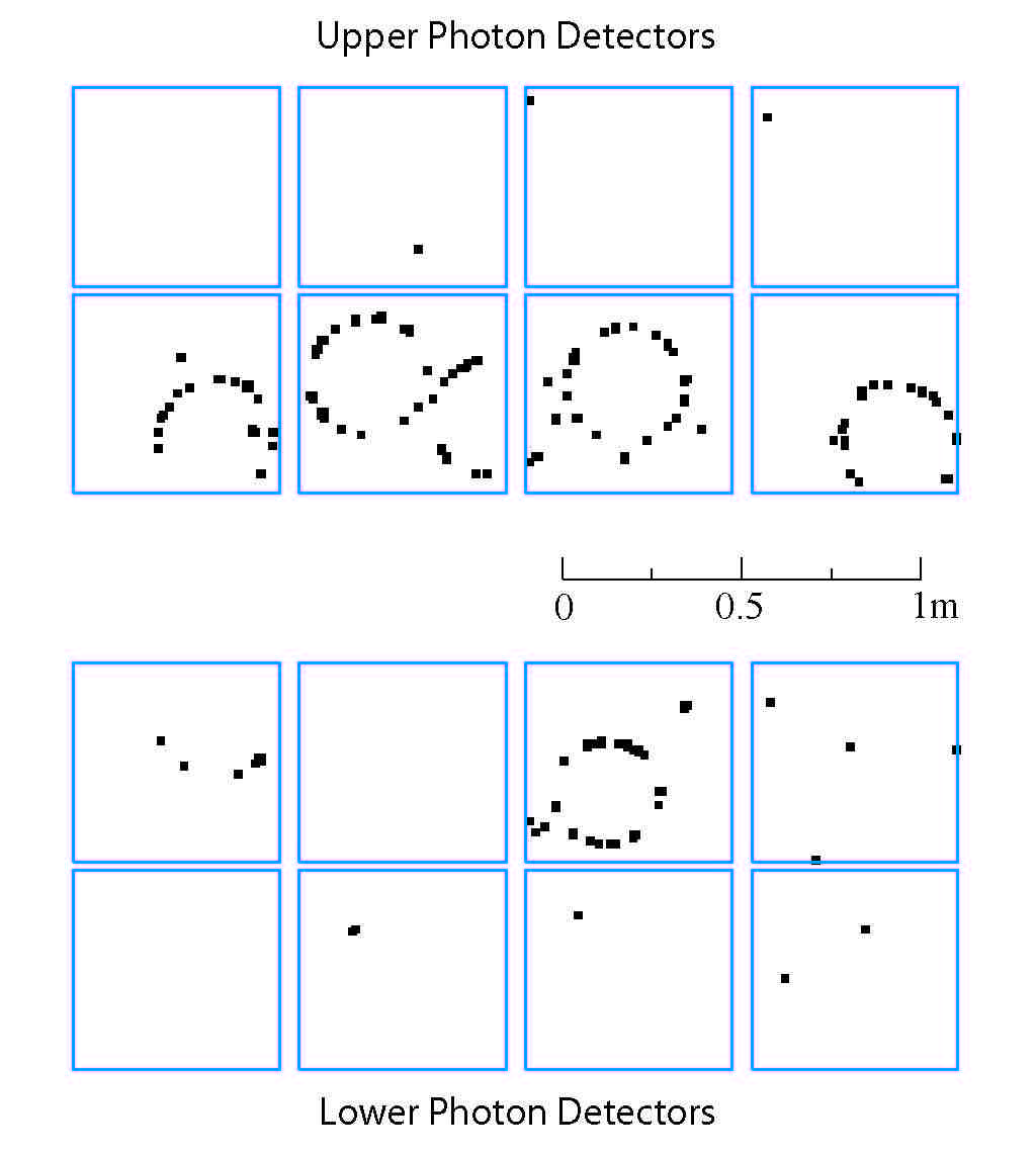
Figure 39: An event from the online event display of COMPASS RICH-1; the squares represent the hits with signal amplitudes larger than a threshold, individually set for each channel.

The COMPASS-GASSIPLEX chips are coupled to an analogue readout system of 82944 parallel channels in total. The chips are housed in 192 identical large front-end boards (BORA board), with 432 input channels each. The BORA boards also house DSP and FPGA processors allowing local data treatment. An average noise level of 1100 electrons r.m.s. is obtained during operation of the detector. The BORA board acquires the data, digitises it in 10 bits, applies threshold and zero suppression and transmits event data. Digitisation is automatically performed after each trigger and data are stored in a FIFO array with up to 128 event capability; this design results in data sparsification downstream of the digitisation stage. The subsequent on-board data reduction is performed in $13\,\mus$ .

The data are transmitted through an optical fibre to the global acquisition system at a data transmission rate of $40\,\mathrm{MB}/\s$. Figure 38 shows the general architecture of the readout system. The main feature of the readout architecture is its distributed computing power, resulting in an easily reconfigurable system. This feature allows a characterisation of all analogue channels by locally measuring and calculating noise and pedestal.

Eight parallel DSP networks allow the BORA control and, in particular, reconfiguring and reprogramming the DSPs and FPGAs as well as acquiring sample events to monitor the overall operation of the system. These networks are handled by DOLINA, a PC resident multiprocessor board housing eight DSPs. A high-level control application software runs on the PC, allowing for a reconfiguration of the BORA control. All BORAs are optoisolated from DOLINA through eight specific optoisolating boards, one for each DSP network, in order to avoid grounding interference between the PC and the detector.

The readout system has been tested up to trigger rates of $75\,\kHz$ with maximum pixel occupancy of 20%.

6.1.5 RICH-1 characterisation in COMPASS environment

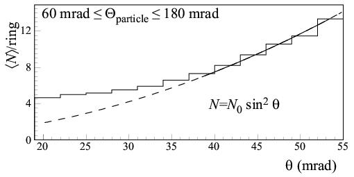
Figure 40: Mean number $N$ of detected photons per particle for the reconstructed ring images, as a function of the measured Cherenkov angle $\theta$. The line is the best fit of the function $N=N_{0}\sin^{2}\theta$ in the range above $36\,\mrad$.

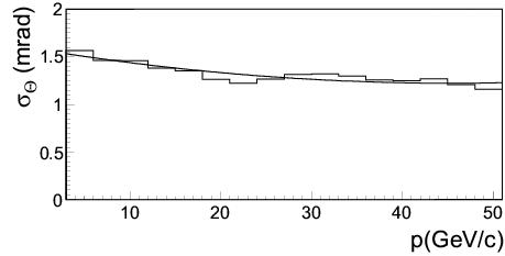
Figure 41: Resolution of the Cherenkov angle for the reconstructed ring images, provided by each single photon, versus the particle momentum for a sample of identified pions.

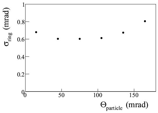
Figure 42: Cherenkov angle resolution for the reconstructed ring images, as obtained from all detected photons, versus the polar angle of the particle track.

Figure 39 shows an example of a RICH-1 event. The pattern recognition allows a determination of some of the most relevant detector parameters: number of photons per event, Cherenkov angle and Cherenkov angle resolution. Figure 40 shows the mean number $N$ of detected photons per particle versus the measured Cherenkov angle $\theta$. The line is the best fit of the function $N=N_{0}\sin^{2}\theta$ fitted in the range above $36\,\mrad$. For smaller Cherenkov angles, the mean number of detected photons per particle is small, and part of the images are not reconstructed, as a minimum number of 4 detected photons per ring is required. The fit clearly indicates that, at saturation, namely at the maximum value of the Cherenkov angle corresponding to $\theta=55\,\mrad$, a mean value of $\sim 14$ detected photons is obtained. The plot in Fig. 41 gives, for a sample of pions, the resolution of the Cherenkov angle measurement provided by each single photon as a function of the particle momentum. At saturation, the resulting resolution is $\sim 1.2\,\mrad$. The resolution on the Cherenkov angle obtained from all the detected photons versus the polar angle of the particle track is presented in Fig. 42. Its value depends on the resolution for single photon measurement and on the number of detected photons, as well as on the signal dilution due to the background. The minimum value is around $0.5\,\mrad$. The achieved resolutions allows pions and kaons separation at $2.5\,\sigma$ level up to $43\,\GeV/c$.

Additional details about the RICH-1 performances are given in Sec. 10.8.

6.2 Muon identification

The muon identification is performed by two detector systems, one in the LAS and one in the SAS part. Both systems are made of a set of tracking stations and a hadron absorber followed by a second set of tracking stations. Such a structure permits to distinguish muons from track segments induced by the typical backgrounds like hadronic punch through from the hadron calorimeters. The muon filtering system in the LAS consists of two stations MW1, separated by a $60\,\cm$ thick iron absorber (Muon Filter 1). In the SAS the tracking behind SM2 is used in combination with a $2.4\,\m$ thick concrete absorber (Muon Filter 2) followed by two stations of MW2 and three MWPC stations (see Fig. 1).

6.2.1 Muon wall 1

The basic element of the MW1 system is the gaseous wire detector called Mini Drift Tube (MDT). The geometry is based on plastic streamer tubes (see reviews in [70, 71]). A modified version of the MDTs with fully metallic cathodes was produced for the COMPASS experiment. The MDT is working in proportional mode. This allows the detector to withstand the high-rate background conditions of the COMPASS experiment.

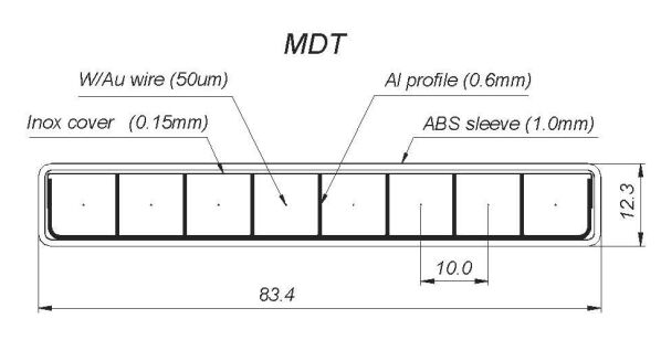
Figure 43: Cross section of a MDT module; all dimensions (except for the wires) are given in millimetres.

An MDT module consists of an eight cell aluminium comb extrusion with a wall thickness of $0.6\,\mm$ covered on top by a $0.15\,\mm$ thick stainless steel foil, gold plated tungsten wires ($50\,\mum$ in diameter) strung in the centre of the cells and an ABS plastic envelope (sleeve) with thickness around $1\,\mm$ to house the interior of the module. The wires are thermally glued to polyethylene plastic spacers (not shown on Fig. 43) at equal distances of less than $1\,\m$ along the length of the MDT to provide electrostatic stability. The wire pitch is $10\,\mm$. The two end plugs are thermally welded at the ends of the MDT, thus forming together with the envelope the gas-tight volume of the module. The plastic envelope also serves for the HV insulation as the negative voltage is applied to the metallic cathode. The anode wires are grounded through the input of amplifiers. Details of the manufacturing and the testing are given in [72, 73].

The schematic view of the MW1 system is shown in Fig. 44. The system consists of two stations separated by a $60\,\cm$ thick iron absorber. Each station has four detectors with two planes of MDTs on both sides. Vertical and horizontal tubes provide the $X$ and $Y$ coordinates, respectively. The outer surface of each station is covered with thin ($1\,\mm$ thick) aluminium sheets for mechanical, electrostatic and noise protection.

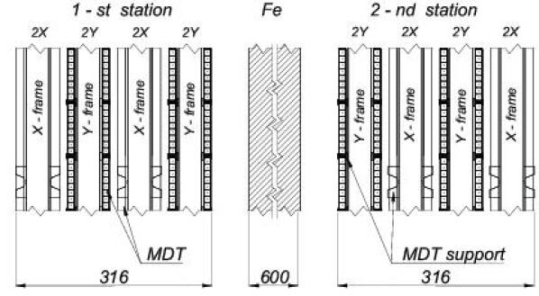
Figure 44: Schematic cross–sectional side view of MW1; all dimensions are given in millimetres. Vertically only part ($255\,\mm$) of the stations are shown.

All frames have a rectangular shape in the $XY$ plane and a hole in their centre matching the acceptance of SM2. The active areas are $4845\times 4050\,\mm^{2}$ (hole $1445\times 880\,\mm^{2}$) and $4730\times 4165\,\mm^{2}$ (hole $1475\times 765\,\mm^{2}$) for the $X$ and the $Y$ planes, respectively. The final planarity of the detector surface was measured to be within $\pm 0.5\,\mm$. The total number of MDT modules in the system is 1056 (8448 wires). The MW1 system provides a measurement of up to eight points per track in each projection with the coordinate accuracy of $10/\sqrt{12}\,\mm$ typical for the $10\,\mm$ wire pitch.

Both MW1 stations have an individual suspension system supported by Muon Filter 1 and the SM2 magnet. It also provides electrical insulation between the iron filter and the stations and serves as a ’clean ground’ for the front-end electronics and its low voltage power supply. The negative HV is applied to the metallic cathode of the MDTs through individual $1\,\MOhm$ resistors.

The gas mixture used is Ar/CO₂ (70/30). It is selected because no ageing effects are observed up to $1\,\C/\cm$, while it is fast enough (drift time is below $150\,\ns$), non-flammable and cheap. The total gas volume of MW1 is $3.2\,\m^{3}$.

The front-end electronics of MW1 consists of an analogue and a digital part. The latter one is located in 6U-crates on the iron absorber at a maximum distance of $7\,\m$ from the analogue cards. The analogue part consists of 264 amplifier-discriminator boards with 32 input/output channels each. The cards use ASIC amplifier [74] and discriminator [75] chips; their design and parameters may be found in Ref. [76]. The digital part [77] consists of 44 digital cards (192 channels each) which are housed in five crates. The digital MW1 card includes six F1-TDC chips (see Sec. 8.3.3) which are used as 32-channel input registers (latch mode).

The whole MW1 system showed very stable performance during nominal data taking conditions. All modules were operated with the same high voltage and threshold settings. Typical values are $2050\,\V$ and $1\,\muA$ for the high voltage and threshold, respectively; the signal amplitudes vary between 5 and $7\,\mu\A$.

The stability was monitored for all 16 planes of MW1. Figure 45 illustrates this for the years 2003 and 2004. Each point in Fig. 45 represents the tracking efficiency averaged over the all 16 planes of MW1. The monitoring was made under the following conditions: only good data taking physical runs were used and the selected events were in fact halo muons with trajectories quasi-perpendicular to the detector planes. The value of the obtained efficiency is typically 91%, close to the geometrical one for the MDT detectors plane of 88.5% (just few percent higher due to the small divergence of the halo muons). The variation of the single plane efficiencies of about 1% diminishes to 0.2% when using the whole MW1 system with at least five (out of eight) points for a track.

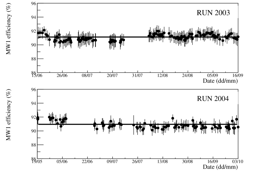
Figure 45: The MW1 averaged tracking efficiency per plane as a function of time (years 2003 and 2004).

6.2.2 Muon wall 2

Muon wall 2 (MW2) consists of two identical stations of layers of drift tubes. Each of the two stations consists of 6 layers with an active area of $447\times 202\,\cm^{2}$ grouped into double layers, each mounted to a separate steel frame. The three double layers have vertical, horizontal and inclined (at $-15^{\circ}$ w.r.t. to the vertical) tubes, respectively.

The stainless steel drift tubes with an inner diameter of $29\,\mm$ and a wall thickness $0.5\,\mm$ were originally designed for the muon system of the DØ experiment [78]. The layout of the tubes in a double layer is shown in Fig. 46. The pitch of the wires in a layer is $33.5\,\mm$. Each tube is inserted into precise guide holes in the frame and fixed with a clamp. The removable fixation allows a replacement of damaged or malfunctioning tubes. The total numbers of tubes in the two stations is 1680.

Figure 46: The layout of the tubes in a double layer of MW2 planes. Dimensions in mm. An imaginary equilateral triangle formed by centres of three adjacent tubes and a common tangent to their interior are shown.

A rectangular hole in each plane of the detector with a size of $1\times 0.8\,\m^{2}$ around the beam is realised using properly shortened tubes. The hole is covered by the MWPC-B (see Sec. 5.3.3) stations, which partly overlap with the sensitive area of MW2.

One end of each tube hosts a high voltage filter with a $1\,\MOhm$ resistor connected with the gold-plated tungsten anode wire of $50\,\mum$ in diameter. The high voltage is delivered to a group of filters through a distribution board mounted on the layer frame. The other end of the tube is equipped with a separate capacitively coupled amplifier-discriminator (AD) connected directly to the signal (anode) and grounding pins of the tube, the latter being soldered to the tube body. The effective threshold of the AD is set to $9\,\fC$. The LVDS outputs of a group of up to 64 ADs are collected with a short (up to $0.5\,\m$) flat cable on a printed circuit which is fixed to the plane frame. This PCB hosts the F1-TDC board (see Sec. 8.3.3) operating in the “standard resolution” mode, and also supplies the low voltage including threshold offset to the ADs.

The gas mixture used, Ar/CH₄ (75/25), is known for a saturated and rather fast drift of electrons, a wide working plateau and stable performance against radiation ageing. The full drift time of $\sim 240\,\ns$ at the working high voltage of $+3\,\kV$ determines the two-track resolution.

The space resolution of the tracking through MW2 includes the intrinsic resolution of the detector itself and the track fitting error, so it is worse for the $Y$ planes, as the corresponding projection measurement is generally less redundant, particularly in this zone of the spectrometer. Fig. 47(a) shows the residuals for a single MW2 layer. The shape of the distribution is approximated with two Gaussians with a common mean: a narrow “core” with a $\sigma$ of 0.53 up to $0.94\,\mm$ (for $Y$ planes) which amounts to 79% to 91% of the entries, and the wide “halo” with a width between 2.0 and $4.8\,\mm$. The spread is mostly due to the irregular spacing of the tubes.

Figure 47(b) shows the two dimensional distribution of the measured time of the hit with respect to the trigger time versus the distance of the reconstructed track to the wire. The correlation is fitted with a linear $R(t)$ relation giving an effective drift velocity of between 5.8 and 6.2$\,\cm/\mus$.

Figure 47: (a) Histogram (thin line) of coordinate residuals for a single MW2 plane with the two Gaussian fit superimposed (thick line). (b) Reconstructed track position with respect to the nominal wire position vs. time for a single plane.

The tracking efficiency for a single plane averaged both over all wires and the wires length is varying between 81% and 84%. It is determined as the ratio of the number of reconstructed tracks having a (registered) hit in the layer not farther than $5\,\mm$ apart from the track crossing, to the total number of reconstructed tracks passing the plane within its acceptance. So, accounting for the ratio of the inner diameter ($29\,\mm$) of the tube to the pitch ($33.5\,\mm$), a value of 83 % corresponds to 96% drift tube efficiency.

6.3 Calorimetry

Two hadron calorimeters and one electromagnetic calorimeter are used in COMPASS setup (see Fig. 1). Both hadron calorimeters are sampling calorimeters using stacks of iron and scintillator plates. They are located before the muon filters. Both hadron calorimeters serve a double purpose in the experiment. They measure the energy of hadrons produced in the target and participate in triggering on inelastic muon scattering events (see Sec. 7.1). ECAL2 is a homogeneous calorimeter consisting of lead glass blocks located before HCAL2. It serves to measure the energy of electromagnetic showers. In addition it was used in the trigger for the measurement of Primakoff reactions with the pion beam (see Sec. 7.2).

6.3.1 Hadron calorimeter 1

The hadron calorimeter 1 (HCAL1) is placed (see Fig. 1) before MW1. HCAL1 has a modular structure, each module consisting of $40$ layers of iron and scintillator plates, $20\,\mm$ and $5\,\mm$ thick, respectively, amounting to 4.8 nuclear interaction lengths. The structure of a calorimeter module and its basic dimensions are shown in Fig. 48 [79]. Monte Carlo simulations for hadrons and electrons were performed in the 10 – $100\,\GeV$ energy range. These particles are almost fully absorbed in such a calorimeter.

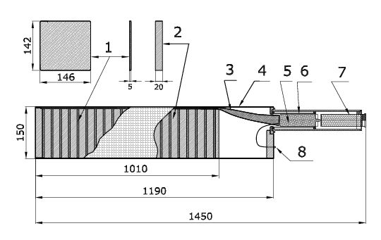
Figure 48: Structure of the HCAL1 module: $1$-scintillators, $2$-iron plates, $3$-light guide, $4$-container, $5$-PMT, $6$-PMT magnetic shielding, $7$-Cockcroft-Walton divider, $8$-optical connector for LED control. Dimensions are in $\mm$.

The 480 calorimeter modules were assembled and framed in a matrix of $28\,\mbox{(horizontal)}\,\times 20\,\mbox{(vertical)}$ with 12 modules removed from each corner. There is a rectangular window of $8\times 4$ modules at the centre of the matrix for the passage of the beam and scattered muons. The outside dimensions of the HCAL1 are $4.2\times 3\,\m^{2}$ and useful surface is $10.8\,\m^{2}$. The calorimeter and its frame are mounted on a platform which can be moved across the beam axis.

The resolution of a sampling calorimeter depends on the qualities of scintillators, light guides and PMTs. The scintillators of HCAL1 have been produced by molding under pressure from granulated polystyrene PSM-115 mixed with P-terphenyl ($1.5\,\%$) and POPOP (1,4-Bis-[2-(5-Phenyloxazolyl)]-Benzene) ($0.04\,\%$). The light from the scintillators is collected by a single flat light guide placed on the open sides of the scintillators with an air gap of $0.6$ – $0.8\,\mm$. The wavelength shifting light guides are fabricated from organic glass (CO-95, CO-120) and painted by cumarine K-30 solved in alcohol. The amount of light emitted and collected from a single scintillator traversed by a minimum ionising particle is enough to produce $4$ – $6$ photoelectrons at the PMT photocathode ($12$-cascade FEU-84-3 PMT). They have multi-sodium photocathodes with quantum efficiencies between $0.18$ and $0.26$ at the wavelength of $460\,\nm$, a large dynamic range, currents up to $5\,\mA$, a typical pulse rise time of $15$ – $18\,\ns$ and a full pulse width of $40$ – $50\,\ns$ at the level of $0.1$ of its amplitude. A Cockcroft-Walton voltage multiplication scheme is used to supply the PMT dynodes with high voltages from the basic $100\,\V$.

The signals from the PMTs are sent via $50\,\Ohm$ cables of about $140\,\m$ length to fast analogue-to-digital converters (see Sec. 8.3.2). Small fractions of the signals are fed into the fast summation system for trigger purposes (see Sec. 7.1.2).

The main characteristics of the calorimeter – linearity of the response versus energy, $e/\pi$ ratio, energy and space resolutions – were determined using the negative hadron and lepton beams at the CERN X5 beam line with energies between $10$ and $100\,\GeV$. The energy resolution of HCAL1 as a function of the energy for pions can be parameterized by $\sigma(E)/E=(59.4\pm 2.9)\,\%/\sqrt{E}\bigoplus(7.6\pm 0.4)\,\%$, with the energy $E$ in units of $\GeV$. A similar dependence is expected from MC simulations. The average value of the $e/\pi$ ratio, calculated from the positions of the electron and pion ADC spectra at the same energy, is $1.2\pm 0.1$. The spatial resolution $\sigma_{\rm x,y}=14\pm 2\,\mm$ was measured by scanning the beam over the central module of a $5\times 5$ matrix and determining of the shower centre of gravity.

The stability during data taking is continuously monitored using a LED system based on a single light emitting diode (LED) of the MARL 110106 type. The light of the LED is distributed and delivered to all $480$ modules by optical fibres about $3\,\m$ long and $1\,\mm$ in diameter. A stable photodiode controls the intensity of the LED. The relative stability of HCAL1 was controlled to 2%. The information is also used to introduce corrections to the detected energy, if necessary.

At the beginning of each COMPASS data taking period, the calibration of the HCAL1 modules is checked by using halo muons. By measuring the amplitude spectra the most probable energy loss of halo muons corresponding to $1.8\,\GeV$ is determined with a precision of $0.1\,\GeV$. In addition the relative signal delays are equalised.

The energy deposited in the calorimeter is compared to the energy (momentum) of the associated particle reconstructed by the COMPASS reconstruction program CORAL. For this purpose the associated particles are combined in ten momentum bins of $0.25\,\GeV/c$ width around the central values $3,5,...30\,\GeV/c$ and the central parts of the corresponding HCAL1 energy spectra are fitted by Gaussian distributions. The positions of the peaks and the corresponding resolution $\sigma$ as a function of the track momentum are shown in Fig. 49. A linear fit $E(p)=A+B\cdot p$ confirms the linearity of the calorimeter energy response and the correctness of the calibration. The constant term $A$ is close to zero within errors and the slope $B$ is equal to $1$ with an uncertainty of about $1\%$.

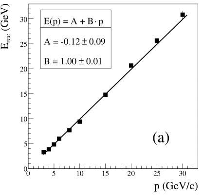
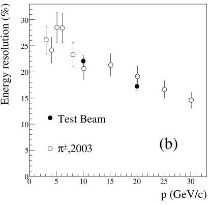
Figure 49: HCAL1 energy reconstruction (a) and energy resolution (b) as function of momentum for identified hadrons (the full symbols denote test beam results).

The efficiency of HCAL1 includes also the efficiency of the cluster search and the energy reconstruction. Thus, the total HCAL1 efficiency depends in principle on the particle energy. For particles with momenta above $5\,\GeV/c$ the efficiency is almost constant and close to $100\%$.

6.3.2 Hadron calorimeter 2

The hadron calorimeter 2 (HCAL2) takes the form of a matrix of $22\times 10$ modules, arranged on a mobile platform. The basic modules are sandwich counters with $20\times 20\,\cm^{2}$ transverse dimensions. The calorimeter has a hole with the dimensions of $2\times 2$ modules to pass the high intensity beam. Two types of modules are used in the detector. Most of them consist of thirty-six $25\,\mm$ thick steel plates, interleaved with $5\,\mm$ thick scintillator sheets. The modules were previously used in the NA12 experiment [80] but the method of light collection from the scintillators and the HV bases for the PMs were modified. The overall thickness of the counters is five nuclear interaction lengths for pions and seven for protons. The central $8\times 6$ cells are filled with thicker modules consisting of forty layers.

The principle of the light collection from the scintillator sheets is presented in Fig. 50. The readout of the scintillation light is done by wavelength shifting fibres of $1\,\mm$ diameter placed in a circular groove in each scintillator sheet. The bundle of fibres from all sheets collects the light onto the S-20 type photocathode of a FEU-84-3 PMT. All scintillator fibre pairs were characterised with a radioactive source and sorted to equalise the module light output. A silicon compound provides the optical contact between the bundle of fibres and the PMT. The computer controlled HV divider is of Cockcroft-Walton type. The PMT signals are measured with the specially designed 12-bit fast analogue-to-digital converters (see Sec. 8.3.2). Small fractions of the signals are fed into the fast summation system for trigger purposes. The timing spread of the signals from different PMTs is compensated with pieces of coaxial cables.

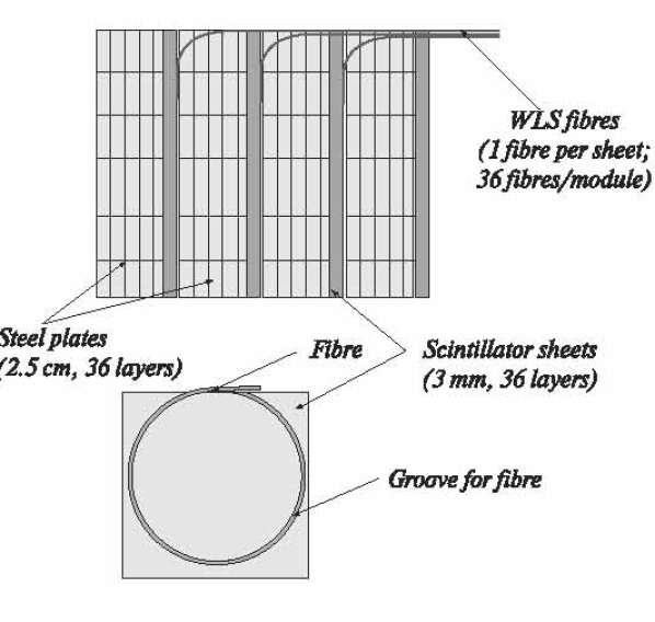
Figure 50: Principle of the fibre light readout of HCAL2, top: side view of part of a module, bottom: front view of a scintillator plate with the fibre readout.

The calorimeter has a light monitoring system common for all modules using a light pulse from a group of light emitting diodes fed to the PMs through fibre light guides. The monitoring system is used for amplification adjustment and control.

As for HCAL1 the characteristics of the HCAL2 modules were determined at the X5 test beam of the CERN SPS using a matrix of $5\times 5$ modules. HCAL2 has a good linearity in the range from $10$ to $100\,\GeV$, the energy resolution is $\sigma(E)/E=(66/\sqrt{E}\bigoplus 5)\,\%$, with the energy $E$ in units of $\GeV$ (see Fig. 51). The uniformity of the calorimeter response was checked by scanning the test beam across the surface of the test setup. It was found to be better than 2%.

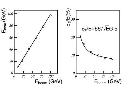
Figure 51: Energy deposition in HCAL2 (left) and energy resolution (right) as a function of the beam energy.

The final calibrations of HCAL2 are carried in the halo of the muon beam of $160\,\GeV$ irradiating the whole calorimeter in the same way as for HCAL1. The efficiency for hadrons is close to 100% for hadrons with energies above $10\,\GeV$.

6.3.3 Electromagnetic calorimeter

The electromagnetic calorimeter ECAL2 in the SAS part of the COMPASS spectrometer consists of 2972 (a matrix of $64\times 48$) lead glass modules with $38\times 38\times 450\,\mm^{3}$ dimensions amounting to 16 radiation lengths that were previously used in the GAMS-4000 spectrometer [81, 82]. A high energy gamma ray (or electron) incident on ECAL2 develops an electromagnetic shower inside the lead glass. The electrons and positrons from a shower emit Cherenkov light on their way through the glass. The amount of Cherenkov light is proportional to the energy deposited in each counter. Each lead glass block is viewed at one end by a PMT which measures the intensity of the light emitted at that counter.

The modules are installed inside a frame, which can be moved vertically and horizontally by $2.5\,\m$ for calibration and maintenance. The ECAL2 platform can be moved on rails along beam axis. A hole of $10\times 10$ modules in the centre allows passage of the beam particles. Two types of lead glasses, TF1 (SF2 class) and TF101 (radiation-hardened by adding 0.2% of cerium), are used in the detector. The radiation-hardened modules (approximately 800) are placed around the central hole. They can tolerate a dose of a few krad [83].

A lead glass module is shown in Fig. 52. The accuracy of the transverse dimension is $0.05\,\mm$. A plastic cylinder enclosing the PMT is glued with epoxy to one end of the glass prism. The PMT is wrapped into three layers of permalloy of $0.1\,\mm$ thickness. It is pressed to the glass by an elastic plate. The optical contact with the radiator is made through silicon grease. The lead glass radiator is wrapped in aluminised mylar. The aluminised side of the mylar is protected with special varnish, which prevents destruction of the reflecting layer and diffusion of aluminium atoms into the glass. The FEU-84-3 PMT with a trialkaline photocathode of S-20 type, $34\,\mm$ in diameter, has been chosen for the counters. About 1000 photoelectrons per $\GeV$ energy deposit are obtained.

Figure 52: A counter of the ECAL2 calorimeter: 1) TF1-000 lead glass radiator, 2) FEU-84-3 PMT, 3) permalloy magnetic screen, 4) quartz fibre to distribute the light pulse of the monitoring system, 5) light guide connector.

Special high voltage dividers have been designed in order to obtain a maximum range of linearity. The divider and the electronics of the computer controlled high voltage supply are described in [84]. For gain monitoring purposes, light pulses produced by a group of LEDs are delivered by a 2 m quartz fibre to the front of each counter. The anode signals of all counters are measured by two types of analogue-to-digital converters, FIADC and SADC (see Sec. 8.3.2).

The calibration of ECAL2 is carried out at the COMPASS experiment with the $40\,\GeV$ electron beam and repeated for each data taking period. The whole calorimeter is moved to expose all modules to the beam and a few thousand events for each module are collected.

The resolutions and linearity were measured previously [81, 82, 85]. For the energy and space resolution $\sigma(E)/E=5.5\%/\sqrt{E}\bigoplus 1.5\%$ and $\sigma(x)=6\,\mm/\sqrt{E}\bigoplus 0.5\,\mm$ were obtained, respectively, with the energy $E$ in units of $\GeV$. The linearity was better than 1% in the energy range from $0.5$ to $40\,\GeV$.

7 Trigger

The trigger system has to serve several purposes: to select event candidates in a high rate environment with a decision time below $500\,\ns$ and minimum dead time, to provide an event time reference and generate strobes for gating some of the analog-to-digital converters, and to trigger the readout of detectors and front-end electronics.

The trigger system is based on fast hodoscope signals, energy deposits in calorimeters and a veto system. Depending on the incident beam — muons or hadrons — and on the kinematics of the reactions different elements are combined to form the trigger signal.

7.1 Muon beam

The COMPASS setup for the muon beam is designed for an as large kinematical acceptance in $Q^{2}$ as possible ranging from $Q^{2}\approx 0$ to the maximum allowed by kinematics. Simultaneously a large range in the energy loss $\nu$ is required.

Events with $Q^{2}>0.5\,(\GeV/c)^{2}$ are mainly triggered by using the scattered muon information only, as it was done in previous muon experiments [11]. The muons are measured in two horizontal scintillator hodoscopes in order to determine the projection of the muon scattering angle $\theta$ in the non-bending plane and to check its compatibility with the target position (vertical target pointing). To suppress events due to halo muons, a veto system is added to the trigger system.

At low $Q^{2}$, in the quasi-real photon regime, the muon scattering angles are close to zero so that target pointing does not work any longer. These events are selected by measuring the energy loss with two vertical scintillator hodoscopes using the bending of the muon track in the spectrometer magnets. At these small angles there are several background processes such as elastic scattering off target electrons, elastic and quasi-elastic radiative scattering off target nuclei and beam halo contributing to the scattered muon signal. The trigger system requires energy clusters in the hadronic calorimeter, which are absent in the background processes. Thus, the quasi-real photon trigger consists of two parts, a trigger on the energy loss by measuring the deflection of the scattered muon in the two spectrometer magnets and a calorimetric trigger selecting hadron energy clusters above a threshold (see Fig. 53). A detailed description of the trigger system is given in [86]. The location of the components of the trigger system in the COMPASS experiment is shown schematically in Fig. 54.

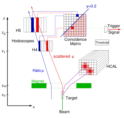
Figure 53: Concept of the trigger for quasi-real photoproduction with high energy loss. The scattered muon leads to a coincidence in the activated area of the coincidence matrix while the halo muon fails to do so. In addition, a minimum hadron energy can be required in the calorimeter.

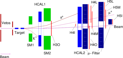
Figure 54: Location of the components relevant for the trigger (schematically). For the true scale refer to Fig. 1.

7.1.1 Hodoscope triggers

In view of the high rates in the central region the hodoscopes of the trigger system are subdivided into four subsystems consisting of two hodoscope stations each, the inner (H4I, H5I), the ladder (H4L, H5L) , the middle (H4M, H5M) and the outer system (H3O, H4O).

With the inner and the ladder system the deflection of the scattered muon in the two spectrometer magnets is estimated by requiring spatial coincidences between the vertical elements in the two hodoscope planes, where the precision is given by the element width of the hodoscopes. The width of the beam at the target, the momentum spread and the multiple scattering introduce an uncertainty into the spatial correlation which has to be taken into account when choosing the minimal relative energy loss $y_{\rm min}$. In addition, muon selection requires an absorber in front of one of the two hodoscopes to reject hadrons and electrons. The effect of the additional multiple scattering can be minimised by placing the absorber ($1.6\,\m$ Fe) directly in front of the second inner hodoscope. The detectors between the two inner trigger hodoscopes have a hole that matches the size of these hodoscopes. A fine grained structure of the two hodoscopes and a muon filter close to the second one is only needed for the $y$ region where the cut is applied. The inner system measuring the $y$ range from 0.2 to 0.5 is therefore fine grained with element widths of 6 and $12\,\mm$, while the ladder system for $y$ between 0.5 and 0.9 uses 20 to $87\,\mm$ strips.

The middle system selects quasi-real photon events as well as DIS events. It uses horizontal planes (21.5 to $30\,\mm$ strips) to detect muons with scattering angles between 4 and $12\,\mrad$. To allow a coarse energy cut, vertical planes (62 and $77\,\mm$ strips) are used. The outer system selects muons up to $Q^{2}\approx 20\,(\GeV/c)^{2}$ by vertical target pointing using 70 and $150\,\mm$ wide elements. The upper limit in $Q^{2}$ is fixed by the size of the gap in the second spectrometer magnet.

The hodoscopes are read out using lightguides and photomultipliers on one or both sides of the elements. The signals are discriminated in customised constant fraction discriminators (CFD). A custom CFD module contains two CFDs and one optional meantimer used for the scintillators with two-sided readout. The signals are fed into coincidence matrices which select only those hit combinations which correspond to muon tracks that either just point back to the target (for hodoscopes with horizontal strips) or that have suffered a minimum energy loss (for hodoscopes with vertical strips).

The discriminator boards holding 32 CFD modules and the coincidence matrices are custom-made VME boards. Special care has gone into the design of the coincidence matrices, which use full custom CMOS chips to achieve excellent timing over the set of 1024 individual coincidences in each $32\times 32$ matrix. To be able to fully exploit the time resolution of the hodoscopes and the coincidence chips, a channel by channel timing compensation stage is included in each of the 64 input channels of each matrix board, using custom-designed CMOS chips with 16 delay and pulse shaping channels with 32 timing steps in a $9\,\ns$ range.

7.1.2 Calorimetric trigger

For hadron detection the signals produced in the two hadronic calorimeters are used to require a cluster with an energy deposition well beyond the value expected for a single muon. In order to correlate an energy deposition with a scattering event on the trigger level a time resolution of order of $1\,$ns of the calorimeter is necessary to reduce the number of accidental coincidences. Also, the trigger has to deal with the very high rate of halo muons of $2\cdot 10^{7}$/s passing through the calorimeter depositing an energy of typically $1.8\,\GeV$. The pulse length of an sandwiched iron-scintillator with wavelength shifter readout is of order 50 ns. Therefore the probability for a two muon pile-up is of order one. The problem can be alleviated by requiring at least one local cluster with an energy exceeding that of a single muon. The size of an energy cluster corresponding to a hadron is of order of one interaction length squared i.e. typically $20\times 20\,\cm^{2}$. With a suitable cluster forming and processing hardware the pile-up problem can be reduced by more than a factor 10.

The signals of $4\times 4$ calorimeter cells are summed in overlapping regions in order to contain complete hadronic showers in one electronic channel while keeping the number of summed channels low in order to limit noise and pile-up of halo muon signals. This is done in two stages: At the back of the calorimeter itself the PMT signals are split into a larger fraction, which goes to the ADCs that measure the individual cells, and a smaller fraction that is summed up in a $2\times 2$ pattern. At the second stage the $2\times 2$ sums are summed up into $4\times 4$ sums. There are four different possibilities to do the summation to cover the calorimeter surface, thus forming four different layers. At the end, every shower is contained in at least one of the sum-of-16 signals of one layer.

Each sum-of-16 signal of the four layers of both calorimeters is discriminated with two CFDs and the discriminated signals are fed into multiplicity units. For the calorimetric trigger in coincidence with a hodoscope trigger, typically a $5.4\,\GeV$ threshold together with a multiplicity $\geq 1$ is used. This threshold suppresses the single muon response by more than $90\,$%. The standalone calorimetric trigger uses a much higher threshold ($16.2\,\GeV$ in 2003, $8\,\GeV$ in 2004) together with a multiplicity $\geq 1$ on two layers. It extends the kinematic range to large $Q^{2}$ values not covered by the hodoscopes and allows an evaluation of the hodoscope trigger efficiencies.

7.1.3 Veto system

Due to the sizeable muon beam emittance and the halo of about $25\,$% (near and far halo see Sec. 3) many triggers in the hodoscope systems are caused by muons not interacting in the target. They can be rejected by adding a veto system to the trigger. It consists of two scintillator counters upstream the target leaving the central region around the beam uncovered. The first large detector (Veto 1, $250\,\cm\times 320\,\cm$) is located at $-800\,\cm$ and the second smaller one (Veto 2, $30\,\cm\times 30\,\cm$) at $-300\,\cm$. Two detectors are needed to veto divergent beam particles passing through the $4\,\cm$ diameter holes in one of them (for illustration see Fig. 55).

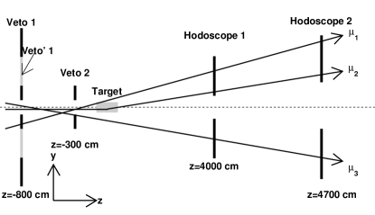
Figure 55: Schematical layout of the veto system. The tracks $\mu_{1}$ and $\mu_{3}$ are vetoed, whereas the track $\mu_{2}$ fulfils the inclusive trigger condition.

This veto system is only fully efficient for tracks with a slope greater than $8\,\mrad$ due to the limited space between the target and the first beam line element. Therefore, a third counter (Veto BL, $50\,\cm\times 50\,\cm$) with a $10\,\cm$ diameter hole was placed further upstream at $-2000\,\cm$ (not shown in Fig. 55). All veto counters are segmented, smaller elements are used close to the beam axis and larger elements in the outside region.

A drawback of the veto system is the dead time associated to it. It is given by the product of the rate of the system and the duration of the time gate during which the veto prohibits a trigger signal. The dead time of the full veto system is about $20\,$% at nominal beam intensity. This veto is only applied to inclusive triggers (middle and outer) which do not require the calorimetric trigger. A subsample of the veto elements was used for the ladder trigger due to the overlap of the trigger hodoscopes with the calorimeters resulting in a dead time of $6\,$%. No veto is needed for the inner trigger. Using the full veto system the middle trigger rate is reduced from 1.4$\cdot 10^{6}$/spill to $18\,000$/spill.

7.1.4 Performance

In 2004 the trigger rates were $14\,000$ and $7\,000$ per spill for the inner and the ladder trigger in coincidence with the calorimeter trigger, $18\,000$ and $9\,500$ for the middle and outer trigger without calorimeter condition and $22\,000$ for the standalone calorimetric trigger.

The efficiencies for all four hodoscope trigger systems were obtained using the standalone calorimetric trigger and yield values of above $99\,$% for the inner and ladder system, $>96\,\%$ for the middle and $>97\,\%$ for the outer system. These lower numbers are due to the suppression of matrix elements which are affected by large backgrounds. The efficiency of the calorimetric trigger was studied in a similar way using events from the middle trigger (without calorimeter condition) with a vertex and more than 3 outgoing tracks. At $\nu\approx 40\,\GeV$ an efficiency of about $90\,$% is reached.

After adjusting the delays at the input of the coincidence matrices, a time resolution of approximately $500\,$ps between the trigger signal and the beam momentum station is achieved for the inner middle and ladder system. For the outer system, due to its larger elements, the resolution is $1\,$ns. The standalone calorimetric trigger has a resolution of $2\,$ns.

The complete veto system has a time jitter of about $1.4\,$ns with respect to the hodoscope systems. Here the time resolution is limited by the use of large scintillator elements of up to $50\,\cm$ $\times$ $100\,\cm$ and elements with small light output due to their operation in the magnetic field of the target magnet.

The efficiency of the veto system was estimated to be about $99\,$%. The resulting trigger purity is about $35\,$% for the triggers using the calorimetric trigger and $15\,$% for the others.

The kinematic range covered by the trigger system is illustrated in Fig. 56. It shows the range in $y$ and $Q^{2}$ for the four hodoscope trigger subsystems and the standalone calorimeter trigger.

Figure 56: The kinematical coverage in $y$ and $Q^{2}$ for the four hodoscope trigger subsystems and the standalone calorimetric trigger. The two lines, $x_{\rm Bj}=1,W=M_{\rm p}$ and $\theta=0$ show the kinematic limits of elastic scattering and forward scattering, respectively.

7.2 Hadron beams

During the 2004 hadron run two different trigger systems have been implemented, one designed to select Primakoff scattering events, and the second to select diffractive $\eta$-meson production. The two systems share a common set of devices that select beam particles pointing to the target and reject events with particles emitted outside the apparatus acceptance. In addition, some specific trigger component are used to select the typical event topologies of Primakoff and diffractive scattering.

Beam particles are detected by the coincidence of two scintillator counters, with a diameter of about $5\,\cm$, centred on the beam trajectory. The Veto 1 system (see Sec. 7.1.3) with a central hole of about $4\,\cm$ in diameter, placed upstream of the recoil veto (see Sec. 4.2), is used to reject beam particles not crossing the target material.

Two additional veto counters made of lead-scintillator sandwiches and located downstream of the recoil veto, are used to reject events with charged particles or photons emitted at large angles and falling outside the acceptance of the electromagnetic and hadronic calorimeters. This condition is needed to precisely define the exclusivity of the reaction in the offline analysis.

Non-interacting beam particles are rejected by means of a system of three small plastic scintillators (beam killers), with a diameter of $5\,\cm$ and a thickness of $5\,\mm$, centred on the beam trajectory and placed between the SM2 magnet and the ECAL2 calorimeter.

The signal of the beam counters is used in anti-coincidence with the sandwich vetos and the beam killers, to form the common part of the trigger logic (common trigger). This information is combined with that of the dedicated trigger devices for Primakoff and diffractive scattering to produce the first level trigger for the COMPASS DAQ.

7.2.1 Primakoff triggers

The Primakoff reaction is characterised by the emission of one single high energy photon in coincidence with the scattered pion. Typical photon energies are above $80\,\GeV$, corresponding to scattered pion momenta below $110\,\GeV/c$. Events with smaller photon energies do not significantly contribute to the measurement of the pion polarisabilities. In order to cover the full energy range of the emitted photons two different Primakoff triggers have been implemented, called Primakoff 1 and Primakoff 2.

In the Primakoff 1 trigger the scattered pion is detected by means of a scintillator hodoscope located in front of the ECAL2 electromagnetic calorimeter (see Fig. 57). The hodoscope is composed of 20 slabs of $6\times 90\,\cm^{2}$ in size and is able to detect pions in the energy range $20-110\,\GeV$. Additionally, an energy deposit larger than $40\,\GeV$ in ECAL2 is required. The calorimeter threshold has been chosen half of the minimum photon energy of $80\,\GeV$ to avoid any bias in the event sample. The Primakoff 1 signal is then made by the coincidence of the common trigger, the scattered pion hodoscope, the ECAL2 signal, and in addition an energy deposit above $18\,\GeV$ in HCAL2.

Events with very high photon energies are selected by the Primakoff 2 trigger. In this second case, the scattered pion hodoscope is excluded from the logic and an higher energy threshold of $90\,\GeV$ is applied to the summed ECAL2 signal. The overall Primakoff trigger is then produced by the logical or of the Primakoff 1 and Primakoff 2 signals.

Typical trigger rates of about $5.8\cdot 10^{4}$/spill for Primakoff 1 and $3.8\cdot 10^{4}$/spill for Primakoff 2 have been obtained during the 2004 hadron run. Due to the overlap in the kinematical region covered by the two triggers, about 20% of the Primakoff events fulfilled both trigger conditions, leading to an overall Primakoff trigger rate of about $7\cdot 10^{4}$/spill.

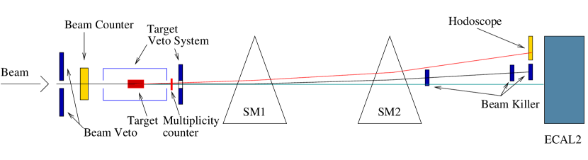
Figure 57: Schematic view of the Primakoff trigger.

7.2.2 Diffractive triggers

In addition to the Primakoff measurement, a test of the diffractive meson production trigger was performed. The trigger was designed to select the $(\eta\pi^{-})$-system, with the $\eta$-meson decaying into $\pi^{+}\pi^{-}\pi^{0}$. These events are characterised by the emission of three charged particles and two photons from the interaction vertex. They are selected by requiring that at least two charged particles hit a scintillation counter read out by a photomultiplier tube and located between the veto box and the downstream silicon telescope. The multiplicity condition is obtained by setting a minimum threshold on the photomultiplier signal. The multiplicity signal is then put in coincidence with the common trigger to form the diffractive trigger. Typical rates of about $2\cdot 10^{4}$/spill have been reached during the 2004 hadron data taking.

8 Readout electronics and data acquisition

8.1 General ideas

The large number of 250 000 detector channels and the total amount of up to $580\,\mathrm{TB}$ data recorded per year demanded to follow new directions in the design of the data acquisition scheme. In order to cope with the high particle fluxes of $2\cdot 10^{8}\,\mu$ per spill of $4.8\,\s$, a typical event size of $35\,\mathrm{kB}$, trigger rates of about $10\,\kHz$ for the muon beam, and a design value of $100\,\kHz$ triggers for the hadron beam, a pipelined and nearly dead-time free readout scheme has been adopted.

An overview of the data flow is given in Fig. 58. The preamplifiers and discriminators are located close to the detectors. The connection of the detector channels depends on the detector type and is described in the corresponding detector chapters. The data are constantly digitised and buffered, where possible directly at the detector front-end electronics, in custom-designed TDC or ADC modules. The synchronisation of the digitising and readout units is performed by the trigger control system (TCS). Upon arrival of the trigger signal the data are transferred via fast links to readout-driver modules named CATCH and GeSiCA. These modules also distribute the trigger signals to the front-ends and initialise them during the system startup. The readout-driver modules combine the data from up to 16 front-end cards and transmit these sub events via optical S-LINK [87] at a maximum throughput of $160\,\mathrm{MB}/\s$ to readout buffers. The data arriving from each link are stored in $512\,\mathrm{MB}$ spill buffer cards. Data from readout modules serving low occupancy detectors are combined by S-LINK multiplexer modules (SMUX) before transmission through the S-LINK. In 2004 the total data transmitted during the spill to the readout buffers corresponds to $230\,\mathrm{MB}/\s$.

The electronics components discussed above, apart from the S-LINK, have been developed specially for COMPASS, while the final event building system is based on high performance PCs and standard Gigabit Ethernet components. The event building takes place during the on- and off-spill time, resulting in an average data rate of $70\,\mathrm{MB}/\s$. These data are recorded on tape remotely at the CERN central data recording facility located in the computer centre.

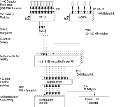
Figure 58: General architecture of the DAQ system. Digitised data from the detector front-ends are combined on the readout modules named CATCH and GeSiCA close to the detectors. The storage of the data during the spill and the event building is performed locally. The data are recorded at the CERN computer centre.

The architecture of the data acquisition system is very flexible and expandable to handle the modifications and upgrades during the lifetime of the experiment. New detectors can simply be added by including the COMPASS standardised readout-driver modules and readout-buffer PCs, while higher rates can be processed by adding more event builders and utilising online filter capabilities.

8.1.1 Ground connections

Most of the readout components in COMPASS measure small and sensitive electronics signals. Specific care was therefore taken for reducing the overall electronics noise of the COMPASS environment. Beyond the conventional safety and protection requirements, the grounding of the COMPASS detectors was designed to minimise ground loops, unwanted couplings and electrical interferences. A star topology of the grounding cables was implemented, all protective grounds being referenced to a unique point of the standard earth of the experimental hall. As a result all electronics and detectors power outlets (high and low voltages, electronics modules, data acquisition racks) were separated from the standard “structure” system and became a part of the “electronics” ground system in the star topology of the COMPASS experimental setup. This topology is complemented by electrical isolation of all electronics racks and detectors. A galvanic isolation from the spill buffers and the subsequent DAQ elements was achieved using optical links. The same requirements were applied to the COMPASS slow-control system.

8.2 Trigger control system

The main function of the Trigger Control System (TCS) is to distribute trigger, time reference and event identification information to the readout-driver modules (GeSiCA and CATCH) and to generate the strobes for gating some of the analogue-to-digital converters.

The TCS employs an optical distribution system which broadcasts information from a single source to a few hundred destinations using a passive optical fibre network. The information is encoded on a serial line with a speed of $155.52\,$MBaud. The clock with which the information is encoded provides a time reference to all frond-end electronics. The network has a star like architecture, where at the top of the system the encoded signal is fanout to ten powerful laser transmitters, then the optical signals are distributed via fibres to different locations in the experimental hall. At every location the light is split to 32 fibres by a passive optical coupler. In 2004 the TCS distributed the information to 150 readout modules.

The trigger control system is based on the encoding method and distribution principles of the Time and Trigger Control (TTC) system developed for the LHC experiments [88], namely the TTCvi encoder and laser module and the passive optical splitters. We have added the TCS controller, the TCS server and the TCS receivers (Fig. 59).

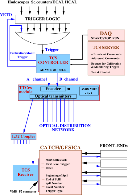
Figure 59: The architecture of the trigger control system.

The controller synchronises data taking with the accelerator duty cycle, it encodes reset and accepted trigger signals, counts the triggers, generates the dead time, generates the event identification information, retransmits the configuration commands from the TCS server and supports the MultiDAQ mode. The TTCvi encoder and laser module encodes the signals from the TCS controller and transmits them optically through the fibre network. The TCS receiver is plugged at the back side of each slot where GeSiCA or CATCH modules are located in a VME crate. The receiver recovers the $155.52\,\MHz$ clock from the incoming data, decodes the data, the trigger and provides this information to the readout-driver module.

The TCS server program communicates with the TCS controller. It provides the command interface between the TCS hardware and the DAQ and monitoring software by means of a client-server protocol via TCP/IP. It ensures protected access to the TCS system and execution of all functions at the right time.

Most of COMPASS front-end electronics are fully pipelined. For some detectors the pipeline principles could not be implemented at the time when the readout electronics were built and a big effort was put towards reduction of the dead time intervals between two consecutive triggers. Due to a mixture of two principles of the readout electronics the TCS generates the dead time with two different algorithms: the minimum allowed time interval between two consecutive triggers and the maximum number of triggers within a certain time interval. The first dead time is needed for the not fully pipelined architecture of the front-ends. The second one is needed for the pipeline readout systems which have a limited depth of derandomised buffers and a limited bandwidth of the data links. During the 2004 data taking the dead time conditions were set to:

• $5\,\mu$s minimum time interval between triggers

• 3 events within $75\,\mu$s

• 6 events within $225\,\mu$s

This setting leads to $5$% dead time at the nominal trigger rate of $10\,\kHz$.

An extensive study of the clock jitter, as one of the most important parameters of the system, was performed. The study demonstrated that the clock jitter between two pairs of the TCS-receivers is about $44\,$ps RMS, which is within the requirements of the COMPASS experiment to allow time measurements with a resolution of $65\,$ps.

8.3 Digitisation

The analogue signals from the various detectors are preamplified and — for time measurements — discriminated close to the detectors, as described in the respective sections of the detectors. The digitisation is also performed in most cases close to the detectors. The gain is twofold: There is no loss of signal quality as no or only short cables are required and the cost for cables is considerably reduced. The specialised RICH readout system based on ADCs and DSPs has been detailed in Sec. 6.1.4. Here follows the description of the ADCs for the silicon and GEM detectors and the two different ADC systems for the calorimeters. All other detectors were read out by a common TDC chip (see Sec. 8.3.3).

8.3.1 ADC for GEM and silicon detectors

The analogue differential output signals of the APV25 chips — which are used for the readout of the GEM and silicon detectors — go via short flat-cables through a repeater card to the ADC card named SGADC. In the case of the GEM detector one ADC card handles all twelve APV chips of a chamber. Each silicon detector is read by two ADC cards: one for the ten APVs on the n-side and another for the eight APVs on the p-side. The analogue signals are digitised by $10\,\mathrm{bit}$ differential ADCs at a sample rate of $20\leavevmode\nobreak\ \MHz$. The digital data of each channel are corrected for the pedestal and are reduced by a zero suppression logic. They are then formatted to $32\,\mathrm{bit}$ words and are sent via optical fibres to a GeSiCA readout-driver module (see Sec. 8.5). Apart from offering a high data bandwidth of $40\,\mathrm{MB}/\s$, the optical fibres also insulate the ADC cards from the readout module. This simplifies the electrical grounding and is of particular importance for the silicon front-end, where, due to the applied depletion voltage, the two ADC cards, that read out one silicon detector, lie on different potentials.

The zero suppression in the ADC cards is based on a threshold cut on the strip amplitudes. Since fluctuations of the baseline of the APVs are observed, the data have to be corrected for this so-called “common mode” noise, before a threshold cut can be applied. The correction is performed at the hardware level and uses a median algorithm based on the data of all channels of one APV chip [89]. A good approximation of the median channel amplitude is obtained from the cumulative distribution of the amplitudes. Due to limited hardware resources this histogram is generated only in a narrow amplitude window around the baseline. In order to position the histogram window the mean amplitude of the 128 channels is used as a first guess for the APV baseline. Hits will obviously pull the average amplitude away from the baseline, but for sufficiently low occupancies the mean lies still close enough to the median. The algorithm is implemented in a FPGA as a pipeline, which is able to process the data of six ADCs in parallel. The pipeline has several stages, which perform the various steps of the zero suppression.

8.3.2 ADC for calorimeters

All COMPASS calorimeters have a fast light signal response, high light yield and a photomultiplier light collection system. They have similar output signal properties, therefore the requirements for the ADC modules are compatible. For the first period of the COMPASS experiment the Fast Integration ADC module (FIADC) was developed. About 3000 calorimeter channels are read out by the FIADC modules. The development of a new Sampling ADC (SADC) started in 2003 when the technological progress in the design of the commercial fast flash ADC chips offered affordable components from the price and power consumption point of view. In 2004 during the hadron pilot run 1000 ADC channels of a newly developed SADC modules were installed and operated. In 2006 the calorimeter setup will be completed and additional 1500 SADC channels will be installed.

Fast Integration ADC: The FIADC module is a 9U VME module, which houses 64 ADC channels. Every channel consists of a gated charge sensitive integrator, which converts the charge to a voltage, and an ADC chip. Upon arrival of the gate signal, which is derived from the trigger signal, the integrator feedback switch opens and the charge is integrated. The integration time is programmable in the range of 100–250$\,\ns$. At the end of the integration time the voltage level at the output of the integrator is converted by the ADC chip to $12\,\mathrm{bit}$ digital information. The digitised information is processed inside a FPGA chip, where the pedestal value is subtracted and the result is compared with the threshold. The values above threshold are combined in one data block. The block header, which includes the module identification and a local event number, is attached to the data block and the complete event information is sent to the CATCH module via a serial HotLink interface with a maximum speed of $40\,\mathrm{MB}/\s$.

The FIADC module has an intrinsic dead time after every trigger. The dead time is the sum of the integration time and the conversion time of the ADC chip. The maximum FIADC dead time in the COMPASS experiment is $400\,\ns$. After digitisation the data are processed in a pipeline mode with negligible dead time. The ADC modules have an integral non linearity of $10\,\mathrm{bit}$ and a typical noise level of $1.2\,\mathrm{ADCchannels}$.

Sampling ADC system: The principle of the SADC is a direct measurement of the signal shape by converting an analogue signal into a sequence of digital values. The digital value represents the amplitude of the analogue signal at a particular time. One of the advantages of the SADC module is a simple implementation of a digital delay line instead of using a coaxial cable for the compensation of the trigger latency. Another advantage is the possibility to use advanced digital signal processing techniques for noise reduction and feature extraction. The SADC read out system consists of two modules, the shaper and the SADC itself.

For the electromagnetic calorimeter the signal behind the photomultiplier tube has a triangular shape with $15\,\ns$ rise time and about $70\,\ns$ fall time. An anti-aliasing filter is required to digitise the fast signals with a $77.76\,$MSPS (mega samples per second) ADC. The shaper employs a very simple circuit of an integrator with a decay time constant of $40\,\ns$. The advantage of the circuit is that it preserves the linear relation between input and output signal integrals and stretches the signal to avoid aliasing problems. One shaper module houses 32 channels and has the same format as the SADC.

One 6U SADC module includes 32 ADC chips which run at $77.76\,\MHz$ with $10\,\mathrm{bit}$ resolution. The ADC chips are preceded by differential amplifiers, which match the signal amplitude to the ADC range and match the input impedance to the cable impedance. The ADC continuously samples the analogue signals and writes data to a ring buffer. The depth of the ring buffer is programmable from 0 to $5\,\mu$s and should match the trigger latency. Upon arrival of the trigger 30 samples are copied to a multi event buffer. Then the data are processed by the zero suppression logic, which accepts only channels with signals above threshold. These data are combined in one data block and transfered to the GeSiCA module via a serial HotLink interface.

The SADC module has a pipelined architecture where every stage of data processing works synchronously with the previous one. The system architecture is intrinsically dead time less. The event rate capability of the system is limited by the bandwidth of the serial interface and the depth of of the derandomisation buffer.

The sampling clock of $77.76\,\MHz$ is derived from the $38.88\,\MHz$ TCS clock. All SADC modules synchronously digitise the analogue signals and this feature allows to measure the signal time with a precision better than $1\,\ns$.

8.3.3 F1-TDC

The requirements for the time measurements widely vary between the different detectors in the COMPASS experiment. The scintillating fibres and trigger hodoscopes produce high rates of up to $10\,\MHz$ and require a high resolution of about $100\,\ps$. On the contrary for the multiwire proportional chambers and the mini drift tubes a time information of $10\,\ns$ is sufficient, but here the large number of channels calls for a cheap solution. The Micromegas, drift chambers, straw tubes and drift tubes needs are in between.

Since no TDC with the high rate requirements and dead-time free readout was available, COMPASS developed its own. The F1-TDC was designed with the flexibility to fulfil all requirements for the different detectors [90]. It provides a cost effective solution, because it is used for all time measurements. The main parameters of the F1-TDC are summarised in Table 10.

The F1-TDC performs digitisation and readout asynchronously and without any dead-time. The phased-locked-loop in each of the F1-TDC is precisely synchronised to the $38.88\,\MHz$ reference clock provided by the trigger control system of the COMPASS experiment. Synchronisation is performed by a signal at the beginning of each SPS accelerator cycle. For each detector channel the arrivals time of the signals, as determined by the combination of the internal phase-looked loop (PLL) and a scaler, are stored for about $1-2\,\mu$s in a 16 or 32 word deep hit buffer. Depending on the number of configured channels per chip, 4, 8 or 32, the digitisation widths are $65\,\ps$, $130\,\ps$ or $4.2\,\ns$, respectively. In case of the 32 input channel operation four channels are combined on one timing unit. Four bits of the time information are reserved to indicate the channels which fired in a programmable time interval. In this so called latch mode operation the time is given for the signal arriving first out of the group of four signals.

The trigger signal is distributed via the trigger control system and the CATCH readout-driver modules to the TDC. Here the hits are selected according to a programmable gate. The resulting time information from the 8 time-measurements units in the TDC are stored in a common output buffer. The data from up to 8 TDC-chips are directly sent via a 8 bit HotLink serialiser chip to the readout-driver modules. Where higher rates are required the 24-bit wide data of four TDC chips are written into a FIFO.

The TDC with its integrated phased-locked-loop and three-wire interface to a digital-to-analogue converter requires only a minimal amount of external components. Thus only small amounts of space is required for the front-end cards located at the detectors.

Table 10: Parameters of the F1-TDC.

Parameter	value
Number of channels	4, 8 or 32
Digitisation width	65 ps, 130 ps, or 4.2 ns
Hit buffer size	32 or 16 hits per channel
Trigger buffer size	4 triggers
Double pulse resolution	typical 22 ns
Hit input level	LVDS, LVPECL or TTL
Edge sensitivity	leading, trailing or both

8.4 CATCH readout-driver modules

To minimise development and maintenance costs we have chosen to unify the readout of all TDC based front-ends as well as the FIADCs for the calorimeter, the ADCs for the RICH and scalers for the trigger. The CATCH readout-driver modules (COMPASS Accumulate, Transfer and Control Hardware) distribute trigger and timing signals to the front-ends, perform the initialisation of the front-ends and serve as a concentrator for the data received from the digitising units of the front-ends. For highest flexibility the inputs are implemented on mezzanine cards, of which four are mounted on each CATCH module (see Fig. 60).

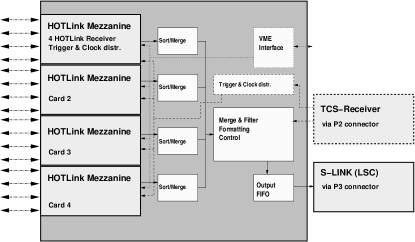
Figure 60: CATCH readout-driver module mounted with for mezzanine cards. Shown are the path of the data (lines), the trigger and synchronisation signals (dashed) and the initialisation (dotted). On the left 16 cables connect to the front-ends.

The hot-pluggable CATCH modules are housed in 9U VME-crates, which provide power and an interface to the CATCH modules via Linux VME CPUs. The configuration of the CATCH and the connected front-ends is performed through the VME interface.

The reference clock, synchronisation signals as well as spill and event numbers are transmitted optically on fibres from the trigger control system to the TCS-receivers (see Sec. 8.2). The TCS receivers are plugged on the backside of the VME backplane at the P2 connector and transmit the decoded information to each CATCH. The CATCH acts as a fan-out and transmits the reference clock and synchronisation signals to the front-ends.

The data arriving from the different front-ends are merged together according to the event numbers. In total 7 FPGAs perform the event sorting, header suppression and framing. The data are stored in intermediate 16k$\,\times\,36\,$bit FIFOs at a maximum throughput of $160\,\mathrm{MB}/\s$.

The complete events are transmitted with a S-LINK transmitter to the readout buffers via optical fibres. Depending on the S-LINK type the maximum transmission rate varies between 100 and 160$\,\mathrm{MB}/\s$. The S-LINK transmitters are plugged on the back of the VME P3 connector. In addition, events are stored on the CATCH in a FIFO, which can be read via VME for test setups with smaller rates and for debugging purposes.

8.4.1 CATCH mezzanine cards

The input side of the CATCH modules is implemented on four exchangeable CATCH Mezzanine Cards (CMC) (Fig. 60). To accommodate all requirements different types of mezzanine cards have been developed [90]. The standard operation mode is to digitise directly at the detectors and transmit the serialised data from the front-ends via 20 m long cables to the Hotlink-CMCs type of inputs. The Hotlink-CMC connects to the front-end via electrical connections, while for the Hotfibre-CMC and HOT-CMC optical connections are used. For detectors which produce high amount of data like the scintillating fibre stations, which are located in the beam, the time measurements are performed on the TDC mezzanine cards (TDC-CMC) located on the CATCH. In the same category falls the Scaler-CMC which counts signals on an event by event basis for normalisation purposes.

Hotlink-CMC: Most front-ends are connected via $600\,\MHz$ Ethernet type cables. Four front-end boards connect to each Hotlink-CMC. Thus to one CATCH 16 front-ends with 64 to 192 channels each are connected, resulting in a concentration of up to 3072 detector channels per CATCH module.

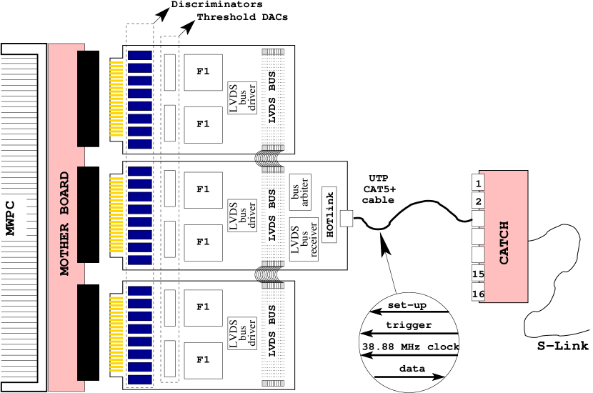
Figure 61: Scheme of the front-end card housing the preamplifier/discriminators, digitising electronics, and the interface to the CATCH via a cable with four twisted pairs of wires.

As an example the scheme of the MWPC front-end cards and its interface to the Hotlink-CMC is depicted in Fig. 61. The signals of the four wire pairs on each cable have been standardised within COMPASS: The CATCH readout-driver transmits to the to the front-end boards the 38.88 MHz reference clock (in differential PECL), the coded trigger and synchronisation signals (LVDS) and the $10\,$Mbaud (TTL) serial initialisation string for the TDCs and discriminators. The front-end sends its 24 or $32\,\mathrm{bit}$ wide data words through a $40\,\mathrm{MB}/\s$ serial link based on a 8b/10b DC balanced standard.

Hotfibre-CMC: For the RICH detector with its special requirements on noise decoupling the Hotfibre-CMC was developed. Here the data are transmitted through optical fibre pairs by making use of transceivers. Since the ADCs do not require the clock signal only the trigger signal is transmitted through the fibre to the front-end. The receiving fibre transfers the data from the front-end in the same coding scheme as the Hotlink-CMC.

HOT-CMC: A new version of the Hotlink-CMC was developed in 2005. It is also based on optical data transmission like the Hotfibre-CMC. But here we implemented the full functionality of the Hotlink-CMC by coding the clock, trigger and initialisation string on a single fibre. Starting in 2006 the readout of the central part of the RICH utilises the HOT-CMC (see Sec. 11.3).

TDC-CMC: The TDC-CMCs measure the signal times of the high rate scintillation fibres and trigger hodoscopes as well as the beam momentum station. On the TDC-CMC four F1-TDC chips are mounted, providing 32 channels of $130\,\ps$ bin width or 16 channels of $65\,\ps$ digitisation width. The LVDS input signals are received from the amplifier and discriminator boards mounted close to the detectors via flat, $20\,\m$ long twisted pair cables.

Scaler-CMC: The scalers measure the rates for the trigger hodoscopes and various counters needed to determine the luminosity. Each Scaler-CMC provides 32 channels of dead-time-free $250\,\MHz$ scalers implemented on a Xilinx Virtex-E FPGA. Both the trigger and the gate input can be adjusted for the timing delays on the cables The Scaler-CMC accepts the same input signals and connection as the TDC-CMC.

In 2004 a total number of 139 CATCH modules mounted in 15 VME crates and equipped with 200 Hotlink-CMCs, 48 Hotfibre-CMCs, 288 TDC-CMCs and 16 Scaler-CMCs were in operation.

8.5 GeSiCA readout-driver modules

The GeSiCA readout-driver is an acronym for GEM and Silicon Control and Acquisition module. Initially the module was designed as a readout module of the GEM and silicon detectors which have a common front-end electronics based on the APV25 chip [35]. These detectors feature high channel density, high occupancy and high data rate. The readout chain of the GEM and silicon detectors is very similar and includes the APV25 front-end card followed by the SGADC card and then the GeSiCA module. Four SGADC cards are attached to one GeSiCA module via high speed serial optical links. One GeSiCA module reads up to 6000 detector channels. The second generation of the GeSiCA, called HotGeSiCA, extends the read out capability. In addition to the SGADC card, it is able to read the SADC front-end modules of the electromagnetic calorimeter.

The tasks of the GeSiCA module are to distribute the TCS clock, the reset and the trigger signals to the front-end cards, to collect the data from the front-end cards and the transfer of these data to the the readout buffer PCs via a S-LINK interface. In addition it provides a slow bidirectional interface for the configuration of the front-end cards.

The GeSiCA is a 9U VME module which has a set of interfaces: the VME interface, four front-end interfaces, a S-LINK interface and the TCS-receiver interface. The front-end interface is a serial optical link with a speed of $40\,\mathrm{Mbit}/\s$ from the GeSiCA to the front-end card and $400\,\mathrm{Mbit}/\s$ backward. The custom protocol provides two independent data channels over this optical link. Via the first channel the front-end card receives the trigger signal and sends back the corresponding data from the detector. The second channel is used for programming the front-end card, for loading firmware, setting thresholds and verifying the status. The second channel is an optical implementation of the I2C protocol. The I2C master is implemented in the GeSiCA FPGA and it is controlled by a user program via the VME interface. The TCS receiver is attached to the P2 connector and provides the TCS clock, the trigger signal and the event identification information.

During the data acquisition the GeSiCA receives data from four front-end cards in parallel. The serial data are parallelised, checked for consistency and put into the FIFO memories. Every event data block is marked by a header and a trailer. The outputs of the four FIFO memories are connected to the merger via a common bus. For every event the merger creates an S-LINK header, which consists of the TCS event identifier, the GeSiCA ID and the block size. The merger sequentially sends the S-LINK header and then four data blocks via the S-LINK card to the readout buffer machine. The total bandwidth of the four front-end interfaces is equal to the bandwidth of the S-LINK interface. Such balanced design minimises the internal buffer sizes and excludes any data losses inside the GeSiCA.

The HotGeSiCA has the same functionality as the GeSiCA module, however it has new features. First of all it is a 6U VME module. The TCS receiver is integrated inside the module and does not occupy the P2 connector. Instead the P2 connector is used for the S-LINK card. The number of the front-end interfaces was increased to eight together with increasing the internal FIFO memory to $512\,\mathrm{MB}$. During production the HotGeSiCA module can be equipped either with optical front-end interfaces or copper connectors depending on the type of the front-end electronics to be attached to the module.

In the 2004 run 15 GeSiCA and HotGeSiCA modules collected data from more than 55 000 channels. For the 2006 spectrometer upgrade of the RICH-1 and ECAL1 the number of modules increased to 24 and the number of attached channels exceeded 120 000 (see Sec. 11).

8.6 S-LINK multiplexer

The S-LINK multiplexer module (SMUX) was developed to minimise the number of readout buffer cards. It allows the data from up to four CATCHes to be transmitted via one S-LINK interface. The number of detector channels read out by one CATCH module varies between 128 and 6912. Many of the CATCH modules read detectors with either low occupancy or low channel density and thus the amount of data transfered by a single CATCH module is relatively small. Therefore it is possible to multiplex the output of several CATCH modules.

The SMUX is a simple 3U card which houses a S-LINK source card, one Xilinx FPGA chip and four parallel S-LINK interfaces. The SMUX is plugged directly to P3 connector of the CATCH module instead of the S-LINK card. Up to three other CATCH modules can be connected with flat cables. During data taking the SMUX expects one data block from every CATCH module for every event. The data are combined in a bigger block and sent to the readout buffer. The module does not need any special configuration, non-active CATCH modules are automatically excluded. In the 2004 beam time 34 SMUX cards were connected to 116 CATCH modules by combining two, three or four CATCHes, depending on the data rate.

8.7 Data acquisition system

In order to match the high rate capabilities of the trigger system and readout electronics, the data acquisition system has to rely on buffering and parallelism. The inputs of the system are the optical fibres coming from the readout-driver modules, carrying fragments of the data pertaining to each trigger. The output are streams of data blocks which correspond to the triggers as issued by the TCS; these are called events. The regrouping of the data streams is called event building and is supported by the spill buffer cards and the DAQ computers which form the event building network, as described in the following three sections.

Due to impurities in the trigger system, the output streams contain events which are useless for analysis. To save bandwidth, storage space and reconstruction time, the output streams are filtered by our Online Filter, which is described in Sec. 8.7.4. The last step in the data acquisition is the transfer of the filtered data to permanent storage and is discussed in Sec. 8.7.5.

The main software used for the COMPASS data acquisition is the Alice DATE package [91], which provides components for event building, run control, information logging and event sampling. It had to be extended by a program including a PCI driver to perform the spill buffer readout. Modifications have been applied to the event building to optimise the input/output and implement an interface to the online filter. The run control is complemented by an electronic logbook developed for COMPASS (Sect. 9.4).

8.7.1 Spill buffer

The spill buffer is an S-LINK to PCI card which is equipped with $512\,\mathrm{MB}$ of memory. The card allows making use of the SPS duty cycle: data are written into the memory during the $4.8\,\s$ beam and are read out via a PCI interface during the full cycle of $16.8\,\s$. This way, the required bandwidth is reduced by a factor of three. In the COMPASS conditions one spill buffer can store the data of 2-3 spills. The DAQ continuously monitors the amount of free memory in the spill buffers and makes a forecast for the next spill. If the amount of free memory does not allow to store the data of the next spill the DAQ either truncates the spill or completely blocks the triggers for the next spill.

The SDRAM memory mounted on the spill buffer is organised in a FIFO like way. The sustained memory access speed is $620\,\mathrm{MB}/\s$ which exceeds the bandwidth of the S-LINK and the PCI by at least a factor of two. The card is fully compliant to the PCI specification.

8.7.2 DAQ computers

In 2004 we used 19 computers as readout buffers, each with $1\,\mathrm{GB}$ ECC SDRAM as main memory, two $1\,\GHz$ PIII CPUs and a 3COM Gigabit Ethernet interface. They have two PCI buses to read in the data on the first 32-bit bus and then transfer it through the second 64-bit bus via Gigabit Ethernet to the event builder computers. This configuration allows a simultaneous reading from the detectors and writing to the event building network without overhead or bandwidth losses. Four spill buffer cards are mounted per readout buffer.

Thirteen computers with two Athlon MP 1900+ processors, $1\,\mathrm{GB}$ ECC DDR-SDRAM and an IDE-RAID with net $640\,$GB per machine were used as event builders. In total $7.68\,\mathrm{TB}$ of disk space are available as buffer in case of problems with tape recording giving a safety margin of about one day. These computers also host the online filter processes.

The greater number of detector channels and the higher trigger rates expected for the data taking from 2006 on require an upgrade of the data acquisition system. Ten new readout buffers with two $3.6\,$GHz Pentium 4 XEON CPUs, and $4\,\mathrm{GB}$ main memory each are being installed. Together with eleven new event builder computers in a similar configuration with 1 TB of disk space each they will supplement the hardware for the event building network. Also dedicated file and database servers, each mirrored and with identical hardware configuration as the new event builder computers will be installed.

8.7.3 Event building network

The data from the individual spill buffers are streams of S-LINK packets, which are multiplexed into one stream of sub-events. The sub-events are then distributed in a round robin fashion to the event builder computers, where the sub-event streams from all readout buffers are multiplexed into streams of complete events, which were on average $35\,\mathrm{kB}$ in size during the muon run in 2004.

All DAQ computers are connected to a set of three 3COM 4900 switches with twelve 1000 BaseT ports and four 1000 BaseSX up-links. These up-links connect the front-end switches to a backbone 3COM 4900SX switch which provides the necessary crosswise connectivity for all DAQ machines. To achieve a balanced configuration, the event builder computers are distributed evenly across the three front-end switches, while the readout buffer computers are connected according to their average output. The stack of switches provides a total number of 36 1000 BaseT ports to connect DAQ computers. The total theoretical bandwidth available for event building amounts to $12\,\mathrm{Gbit}/\s$.

8.7.4 Online filter

The online filter increases the purity of the triggers and allows for a cost effective reduction of the amount of tapes needed for recording. For the physics programme with hadron beam the online filter is required to reduce both the bandwidth needed for transferring the data to the computer centre as well as the bandwidth needed to record the data on the tape drives. In addition one profits from a reduced CPU time for the reconstruction of the data.

The basic unit for the online filter is the complete event as it is produced by the event builder process. To facilitate the relocation of the filtering task to its own dedicated computing farm at a later stage, the event stream produced by each event builder is sent via socket I/O to the online filter process, which up to the beam time of 2004 ran on the same computers as the event builder processes. The filtered event stream is written to the local hard disk arrays to await the asynchronous transfer to the central data recording services.

At a trigger rate of $10\,$kHz, a particle extraction duty cycle of $30$% and with 13 event builders sharing the load, the allowed average decision making time is $4\,\ms$ per event. This constrains on the present hardware the event analysis in two ways. First, only partial decoding of the data is possible. Second, tracking of charged particles is impossible in regions where a magnetic field is present. This also excludes the use of information from the RICH detector in the filter decision.

For the two physics programs, two filter algorithms have been developed. In the muon programme the presence of a reconstructed beam track is required. For this the silicon microstrip and scintillating fibre detectors upstream of the target together with the beam momentum station must have recorded the a sufficient number of hits from the beam particle. The algorithm is based on the coincidence between the trigger time and the times measured by the aforementioned detectors, respecting their different time resolutions and allowing for the redundancy of the detector systems. Inevitable changes in the timing of the detector signals due to changes in the environmental conditions are compensated by an online re-calibration process. In 2004 we achieved a rate reduction by $23$% with an associated inefficiency of $0.4$%.

For the hadron pilot run of 2004, the Primakoff trigger has not been filtered, while the diffractive trigger was subject to a multiplicity cut. The hits recorded by the silicon microstrip detectors downstream of the target are filtered by the same coincidence algorithm as in the muon program’s case. The truncated mean of the hits per detector plane then is a good approximation of the track multiplicity after the target. Requiring this quantity to be greater than one lead to a rate reduction of $45$% for the diffractive trigger.

Presently these performance was enough, for the future physics programme larger reduction rates will be achieved by the implementation of a dedicated filter farm.

8.7.5 Central data recording

During data taking, the data flow is split in files of $1\,\mathrm{GB}$ maximum each, which are written on the event builder disks. In parallel, headers of each event are read and written to a metafile for later storage in an Oracle database. The files are copied in parallel TCP/IP streams via a dedicated Gigabit link to disk servers located at the CERN central computer centre. These disk servers are part of the CASTOR hierarchical storage system [92]. A specific configuration of CASTOR has been created for COMPASS and 6 tape writers are reserved for the copy of the data files to tape. The configuration has been optimised over the COMPASS data taking years to finally reach performances of more than $8\,\mathrm{TB}/\mathrm{d}$, a rate close to the one needed for the LHC experiments ATLAS and CMS. When the copy to tape of a given file is confirmed, its deletion is then authorised and takes place when the space in the event builder disk is running low. In parallel, when the data file is stored on tape, the corresponding metafile is used to fill the Oracle database with information on the run and on each event. The database, for performance reasons spread over 9 computers, allows the reconstruction software to have a direct access to each of these events, using selection criteria like trigger type or event number.

8.7.6 Performance

The maximum sustained data rate which has been recorded was $8\,\mathrm{TB}/\mathrm{d}$ during the hadron pilot run, which corresponds to $740\,\mathrm{Mbit}/\s$. The limiting factor was the network link to the computing centre, a single $1\,\mathrm{Gbit}/\s$ connection. Data rates of up to $1.5\,\mathrm{Gbit}/\s$ have been achieved during tests without transferring the data to permanent storage.

9 Detector control and monitoring

The detector control and monitoring systems provide a user interface to control the majority of the hardware parameters of the COMPASS apparatus and ensure that the quality of COMPASS data stays at a high level during data taking. Different aspects of the experiment are constantly monitored: the operation of the front-end electronics and the read-out chain, the stability of the beam characteristics and the counting rate level of the different triggers. The consistency and correctness of the data flow produced by the front-ends is not sufficient to guarantee a reliable operation of the detectors. This information has to be complemented by more detector-specific parameters, like supplied voltages and currents, hit profiles, time or amplitude information or noise spectra. The online monitoring is performed on data provided on the fly by the DAQ system.

The various tools used to control and monitor the COMPASS spectrometer are described below.

9.1 The detector control system

The main task of the Detector Control System (DCS) is to provide a complete and user friendly interface for setting and reading back all the relevant parameters for the operation of the various detectors and data acquisition elements, like high voltages, low voltages, VME crate status, gas pressures and mixtures, temperatures and magnetic fields. A software package allows to check and modify all parameters remotely, thus minimising the need to access the experimental hall.

The DCS architecture (see also Fig. 62) is composed of three layers. The supervisory layer, based on the commercial package PVSS-II [93], provides the graphical user interface for accessing and monitoring the hardware parameters. The front-ends layer include the various software drivers specific for each hardware element. It provides the supervisory layer with a common communication interface to access the hardware. Whenever available, existing commercial drivers have been used, while custom drivers have been developed for unsupported hardware modules. The hardware elements (crates, sensors, gas systems, etc.) form the devices layer.

Such a modular architecture allows to control a large variety of devices in a coherent and transparent way:

• control of crates and power supplies;

• monitoring of voltages and currents in crates and power supplies;

• control of high voltage channels;

• monitoring of temperature, humidity, pressure and magnetic field in specific points of the experimental hall, sub-detectors and magnets;

• monitoring of gas fluxes and mixtures in gaseous chambers.

9.1.1 The devices layer

The DCS controls a large number of devices that are spread over about $200\,\m$ along the spectrometer and in the beam tunnel. A total of about 2000 high voltage (HV) and low voltage (LV) channels are constantly monitored by the system. The HV power supplies are mainly different types of CAEN [94] modules housed in various main frame models. These main frames also contain part of the LV power supplies. Most of the CAEN main frames are connected in daisy chains to 5 CAENET buses, while Ethernet is used for a few very recent models. Several ISEG [95] HV modules and the power supplies of the WIENER [96] VME crates are controlled via standard CANbus lines.

ADC readings for analogue measurements are performed using the multi-purpose I/O system Embedded Local Monitor Board (ELMB) [97] developed at CERN for the ATLAS experiment. A total of 28 ELMBs are used, providing the readout of 800 analogue sensors.

The various gas systems are controlled by Programmable Logic Controllers (PLCs), that act on mass flow meters, pressure sensors and valves to ensure constant and correct gas flows and mixtures. The parameters relevant to monitoring are sent via serial connection to one of the front-end DCS computers.

9.1.2 The front-ends layers

OLE for Process Control (OPC) [98] servers exist for the majority of modules used in COMPASS. Wherever a commercial solution was not available, custom drivers have been developed in collaboration with CERN, making use of the SLiC [99] framework developed at CERN and using OPC or Distributed Information Management (DIM) [100] protocols. For example, the CAENET-based high voltage system is managed by a SLiC DIM server with tunable read cycle speed for each of the controlled parameters. A fast cycle is used for the monitored voltages, currents and channel status with speeds of $10-20\,\ms$/channel. This allows a fast detection of high voltage trips and failures. A slow cycle, with a readout period of 3 minutes, is used for the read-back of setting values.

The OPC and DIM servers are running on Windows and Linux computers. The monitored values are exported to clients in the form of lists of items. Clients subscribed to a certain list are notified whenever an item changes its value or status. This event-driven protocol minimises the network traffic in the DCS.

9.1.3 The supervisory layer

For the supervisory layer the software package PVSS-II has been extended at CERN with the JCOP-Framework [101], which implements the functionalities specific to high energy physics experiments.

The supervisory layer consists of a core application and several OPC and DIM clients for the communication between the application and the front-ends layer. The application provides a graphical user interface for visualisation and control of the parameters, and an interface to the dedicated database were the monitored values are stored together with their time stamps.

An alarm system provides acoustic and visual alarms when critical parameters fall outside predefined boundary levels, or when hardware failures are detected. The alarm system reacts to a wide variety of events: high voltage trips, gas system failures, temperature and magnetic field changes and crate failures. In addition, the trend of stored parameters as a function of time can be displayed via the main user interface, thus making it easy to recognise slow drifts or locate in time changes in the parameter values.

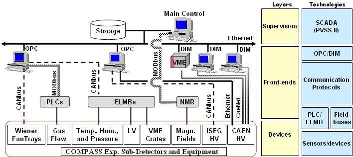
Figure 62: The architecture of the Detector Control System.

9.2 Beam and trigger stability

The stability of the beam parameters, like the intensity and the position at the COMPASS target, is an essential requirement for the measurement of small physics asymmetries. Slow drifts of the beam characteristics can occur, as well as significant variations from one spill to the other. Therefore, a continuous monitoring of the beam parameters is needed.

The beam and trigger monitoring software tool checks the beam current and position, and the rate for each trigger type on a spill-by-spill basis, and stores the read values into a local MySQL database [102]. Trigger rates normalised to the beam current are also computed to detect beam changes and failures of the trigger system. The trend of those parameters over the last few hours is constantly displayed.

9.3 Data monitoring

The read-out chain and the front-end electronics of the detectors are monitored by a software tool named MurphyTV. Samples of events are read on the fly during the data taking to monitor the data quality. Failures of the read-out chain are detected by error words generated by the electronic boards themselves, or by inconsistent formats of the data structure (missing headers or trailers, missing part of the data, incoherent event numbers in different portions of the same event, etc.). MurphyTV reports these errors in a graphical user interface.

A software package named COOOL [103] has been designed to read COMPASS raw data streams and to produce different sets of ROOT histograms [104] for each detector plane or group of detector planes. The COOOL program provides a graphical user interface that allows the user to interactively browse through the histograms and print them for future reference. The histograms are saved into a ROOT file upon program termination; the raw detector information can also be stored in the form of a ROOT tree, to allow the quick re-processing of the data. The generated histograms, like counting rate profiles, time spectra, signal amplitude distributions, allow the detection of several types of failures, like high voltage failures, low voltage failures, large electronics noise, or failures of front-end electronics cards. For each histogram, a reference distribution is plotted on top of the current one, thus providing a quick comparison with the nominal detector behaviour. The COOOL package is also extensively used for detector commissioning and running-in.

9.4 Run logbook

To keep track of the data taking and of the conditions of the experimental setup a web-based logbook, connected to a MySQL database for the permanent storage and easy searching of the comments and annotations, was developed for COMPASS.

A large variety of information is stored automatically at the beginning of each data run (equivalent to 100 or 200 SPS spills), thus providing a complete overview of the data taking conditions of each single data run. In addition, some data quality checking and online monitoring tools (see Sec. 9.3) process a sub-sample of the collected data, to produce detector and DAQ performance histograms.

The list of automatically stored pieces of information is the following:

• information from the DAQ system

• information provided by the shift crew

• trigger information

• beam line information

• status of the COMPASS target

• currents of spectrometer magnet SM1 and SM2

• a ROOT file containing the COOOL histograms

• detector specific information extracted from the COOOL histograms

• text output from the MurphyTV software which monitors errors coming from the front-end electronics

All stored information can be retrieved, searched and displayed through a web server.

10 Event reconstruction and spectrometer performances

The huge amount of data (about $350\,\mathrm{TB}/\Year$) collected by the experiment requires the availability of sufficient computing power to reconstruct the events at a rate comparable to the data acquisition rate. The required CPU power is estimated to be 200k SPECint2000 units, which are provided currently by 200 Linux Dual-CPU PCs out of the CERN shared batch system. Event reconstruction is performed by a fully object oriented program (CORAL) with a modular architecture and written in C++. The schematic representation of the reconstruction software, describing the various steps performed and their mutual connections, is shown in Fig. 63.

Figure 63: Schematic representation of the COMPASS reconstruction software.

The input of the reconstruction software is represented either by the raw data collected by the experiment, or by the output of the Monte Carlo simulation software (see Sec. 10.5). The data files produced by the COMPASS acquisition software contain the raw information from the detectors, digitised by the front-end electronics. Two initial processing phases are needed to prepare the input to the track finding algorithm. In the first phase, called decoding, the information on the fired detector channel (either wire, pad, or cell, depending on the detector type) is extracted from the raw data. In the second phase, called clustering, detector channels that are fired by the same particle are grouped together. For some detectors weighted centre-of-gravity algorithms are applied to get a better determination of the particle parameters. During the clusterisation phase, the information on the geometrical position of each detector in space is used to calculate the coordinate of the cluster in the main reference system of the apparatus. The geometrical position of each detector plane is retrieved from files that are generated either by the alignment procedure (see Sec. 10.2) or by the Monte Carlo package. The clusters are then pre-selected on the basis of the time information.

When Monte Carlo data files are processed, the decoding phase is replaced by a digitisation phase, in which the response of the detector is simulated and hits are produced on the basis of the particle trajectory and detector resolution.

After clusterisation, charged and neutral particles are reconstructed and particle identification is performed. The information from tracking detectors is used to reconstruct the trajectories of the charged particles through the spectrometer and to determine their momenta, as described in Sec. 10.1. Hadron calorimeter clusters are used to separate muons and hadrons; electromagnetic calorimeter clusters measure the energy and impact coordinate of photons and electrons (see Sec. 10.9). Hadron identification is performed by the RICH-1; a dedicated software package which combines information from the RICH photon detectors and from reconstructed tracks and momenta, is used to calculate the most probable Cherenkov angle and to assign probabilities to all possible particle hypotheses (see Sec. 10.4).

A vertex finding procedure is applied to all reconstructed tracks, in order to identify the primary interaction point and subsequent decays of neutral particles, as described in Sec. 10.3.

The result of the reconstruction phase (track parameters, vertices, calorimeter clusters, PID probabilities, detector hit patterns, etc.) is stored into output ROOT [104] trees, called mini Data Summary Tapes (mDST), that are distributed to home computing centres and serve as input for all the physics data analyses. The data reduction factor between the input raw data and the output mDSTs is about 100. Large DST files, storing the detector digits and clusters in addition to the tracking, vertex, and PID information are also created and kept at CERN on tape.

The following subsections describe the main steps in the event reconstruction and give a summary of the corresponding performances.

10.1 Track and momentum reconstruction

The track reconstruction algorithm (TRAFFIC/TRAFDIC) is divided into three phases corresponding to pattern recognition (i.e. finding track segments in the various zones of the spectrometer), bridging (i.e. connecting track segments from several distinct zones to build full tracks), and fitting (i.e. computing the best estimators for the parameters of the reconstructed tracks).

The pattern recognition selects sets of clusters consistent with track segments. To that end, the spectrometer is divided into 5 zones along the beam, where track segments are expected to follow approximately straight lines. The five zones comprise the regions upstream of the target, from target to SM1, from SM1 to SM2, from SM2 to the second muon filter, and downstream of the second muon filter. The first one is only used for beam tracks: tracks reconstructed in the beam telescope are extrapolated upstream and associated, on the basis of time and position, to momentum measurements performed in the BMS (see Sec. 3.3).

Reconstruction is first performed in projections. For this purpose the detector planes in each zone are divided into groups having the same orientation, thus measuring the same projection of a track. A pivot-plane algorithm is used to search for track segments in these projections. In this approach, each pair of detector planes is used successively as a pair of pivots. Each pair of clusters from the pivot planes is used to define a straight road, thus associating clusters from all other planes. At each successively encountered detector, the road width is adjusted to take into account the detector resolution. This projection search is performed for each projection. A pre-selection of candidate track projections is then performed, based on the number of clusters, and taking into account its variation as a function of the track angle.

In the next step, all projections are combined to produce space track segments. The search combines track segments taken from pairs of projections to open a road in space; clusters from all detectors in all projections are then collected within this road. For each detection plane, the position corresponding to the measured coordinate is assigned to the cluster, and a check whether the track impact point is within the sensitive area of the corresponding detector is performed. All track candidates are then compared to a dictionary of possible tracks through the COMPASS spectrometer. This dictionary is organised as a look-up table, thus increasing the speed of the fitting procedure.

The building of full tracks out of the track segments found in the preceding phase proceeds sequentially, first via straight line fit, and then via bridging (connecting track segments) of two adjacent zones. The successfully combined track segments are then ordered according to a quality function (QF) based on the $\chi^{2}$ and the number of hits associated to the track. The combination with the best QF is retained, while combinations re-using one of the previously accepted segments are discarded. The process is iterated until the list is exhausted.

In the final phase of the tracking algorithm, magnetic fields and material maps are used to get the best estimates of the track parameters ($x$ and $y$ positions, $\mathrm{d}x/\mathrm{d}z$ and $\mathrm{d}y/\mathrm{d}z$ slopes, inverse momentum $1/p$) and their error matrix. For this purpose, the Kalman fit method is used [105, 106]. The fit starts from the first cluster of the found track. The track parameters are updated by this measurement and propagated to the next detector surface. This process is repeated for all clusters belonging to the track. The Kalman fit is performed twice, first in the downstream and then in the upstream direction, in order to provide the track parameters at the first and last measured point of the track.

The momentum of low energy particles emitted at large angles, and therefore not entering the SM1 aperture, is calculated from their trajectory in the fringe field of the magnet, although with smaller accuracy. These are called fringe field tracks [8].

Apart from spatial measurements (cluster coordinates), a number of COMPASS detectors also provide time information (cluster time) with respect to the time of the trigger signal. As those measurements are completely independent from coordinate measurements, the time component is not included in the track parameterization but a weighted mean time is calculated separately. This track time information is important for rejection of pile-up tracks, beam momentum determination, trigger system performance studies, etc.

The list of tracks obtained at the end of the track reconstruction procedure is then scanned to search for the muon outgoing from the primary interaction (scattered muon). A track is identified as a scattered muon if it corresponds to a positively charged particle, and if its trajectory is compatible with the hodoscope hits as given in the trigger matrix. For the standalone calorimetric trigger (see Sec. 7.1), a minimum number of hits is required downstream of either the first or the second hadron absorber. In addition, the muon track candidate must cross the entrance and the exit of the polarized target at a distance smaller than $5\,\cm$ from the beam axis. The beam track and the fringe field tracks are excluded from the search.

10.2 Alignment procedure

The alignment procedure determines the detector positions in space by minimising the $\chi^{2}$ of all tracks simultaneously. Initially tracks are reconstructed using detector positions determined by a geometrical survey. The minimisation of the $\chi^{2}$ is based on the analytical inversion of a huge sparse matrix, using the Millipede program described in [107]. The optimised parameters are: $i)$ the position of the detector centre, $ii)$ the rotation between the detector coordinate system and the global coordinate system, $iii)$ the effective detector pitch, i.e. the distance between adjoining wires or pads. The procedure is iterated until the changes in the detector positions become negligible compared to their resolution.

The adjustment of detector parameters is first done using data samples, collected with the spectrometer magnets switched off, so that straight trajectories through the spectrometer can be assumed, and then refined using standard data. The alignment procedure is repeated after each long interruption of the data taking and each time some detector has been moved.

10.3 Vertex reconstruction

The last phase in the event reconstruction is the location in space of the primary interaction or of the two-body decays of neutral particles (so-called $V^{0}$ vertices). Here the aim is to get the best estimate of the three coordinates of the vertex position from which each track is assumed to originate, of the three components of the momentum vector of each track at this vertex, and the corresponding covariance matrices.

A first approximation of the primary vertex is obtained by computing the average Point Of Closest Approach (POCA) between one beam track and all possible outgoing tracks. All tracks having a POCA too far from the approximated vertex position are discarded; an exception is represented by the scattered muon, which, if present, cannot be removed from the vertex.

A vertex is called primary when it contains a beam track. Since more than one beam track can exist for one event, as many primary vertices as the number of existing beam tracks can be reconstructed in this phase; the selection of the best vertex is performed later at the level of physics data analysis.

The tracks surviving the initial selection are used to perform the fit of the vertex position by an inverse Kalman filter algorithm. During the first iteration, all tracks are used to estimate the parameters of the vertex, and the relative $\chi^{2}$ contribution of each track to the fit is computed. If the largest $\chi^{2}$ contribution exceeds a threshold value, the corresponding track is removed from the list and the procedure is iterated once more. However, neither the reconstructed beam track nor the scattered muon track can be removed from the vertex. The algorithm stops when all remaining tracks survive the $\chi^{2}$ selection.

The procedure described above may fail if the initial list of tracks contains a large number of fake tracks. In such a case the initial vertex position may be estimated to be too far from the real one, resulting in a rejection of the good tracks. In order to avoid this difficulty, a recovery procedure is applied at the end of the vertex fit phase. The unassigned tracks are re-inserted in the list one by one, and the vertex fit is re-calculated each time. A track surviving the $\chi^{2}$ selection is then finally re-assigned to the vertex. The recovery phase ends when all unassigned tracks have been checked.

The distribution of reconstructed primary vertices along the beam axis, for events with a $Q^{2}>1\,\GeV^{2}/c^{2}$ (Fig. 64 (top)), shows clearly the structure of the target cells, in good agreement with their real position. Vertices reconstructed outside the cells correspond to interactions with liquid helium or some other target component.

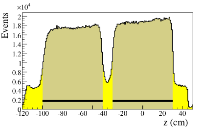
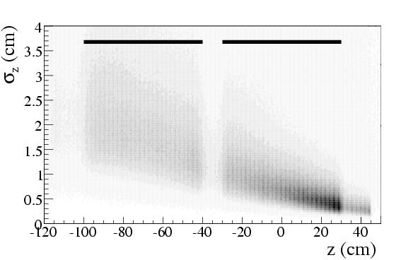
Figure 64: Distribution of the reconstructed vertex position $z$ along the beam axis (top); distribution of the error $\sigma_{z}$ vs. $z$ (bottom). The solid lines show the position of the target cells.

In the direction perpendicular to the beam axis, the primary vertex coordinates are determined by the Kalman filter with an accuracy of about $0.1\,\mm$. Along the beam axis the resolution depends on the production angle of secondary particles, which is limited by the opening angle of the target solenoid, and increases from about $5\,\mm$ at the downstream end of the target to $25\,\mm$ in average at the upstream end (Fig. 64 (bottom)). The vertex resolution, estimated using Monte Carlo simulations that include beam halo and pile-up background, is compatible with the resolution determined with the Kalman filter method. The number of tracks not connected to any physical vertex is smaller than 3%.

Secondary vertices are reconstructed inside the target and several meters downstream, so that nearly all $K^{0}_{S}$, $\Lambda$ and ${\overline{\Lambda}}$ decays into charged particles are observable. The $V^{0}$ vertices are searched by combining all pairs of tracks with opposite charge, regardless of their association to the primary vertex. The most probable decay position, the track parameters at the vertex and the corresponding error matrices are calculated using the Kalman filter technique. For decays occurring downstream of the target, the mass resolution is found to be $7.6\,\MeV/c^{2}$ for the $K^{0}_{S}$ and $2.5\,\MeV/c^{2}$ for the $\Lambda$ and ${\overline{\Lambda}}$ (see Fig. 65).

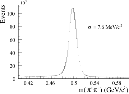
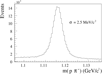
Figure 65: Reconstructed invariant mass of $V^{0}$ decays, in the hypothesis of $\pi^{+}\pi^{-}$ decay (top) or $p\pi^{-}$ decay (bottom), respectively.

10.4 The software package for the analysis of RICH-1 data

The pattern recognition and Particle Identification (PID) with RICH-1 is performed inside CORAL by a package called RICHONE [108]. The raw RICH-1 data provide the coordinates of the Photon Detectors (PD) pads with signal above threshold and the signal amplitude; this information is combined with the particle trajectory at the RICH entrance known from track reconstruction. At first a clustering procedure is applied to the hit pads. The photon Cherenkov angle is reconstructed according to a recipe from the literature [109]: knowing the reconstructed particle trajectory and the coordinates of the detected photon at the photon detectors, assuming that the photon is emitted at the mid point of the particle path in the radiator, an estimation of the Cherenkov angle is obtained for each detected photons. The uncertainty in the photon emission point corresponds to the spherical aberration of the image. The best estimate of the measured Cherenkov angle is the mean value of all the Cherenkov angle estimations obtained. This algorithm is at the base of both RICHONE particle ring recognition and PID. The ring recognition is mostly used to monitor all the properties and the performances of the RICH, like PD and mirror alignments, photon and ring angular resolution, PID error calibration, ring reconstruction, pseudo-efficiency, and also for a first approximation ${\chi}^{2}$-based PID. The PID in use is based on a likelihood method which includes several ingredients. All the photons, within a large fiducial area, are taken into account and compared to the mass hypothesis. An accurate cluster background description is obtained from the distribution measured on the PDs themselves. A Poissonian probability, taking into account the expected number of detected photons, as a function of the particle mass and momentum and of the detector acceptance (dead zones), is also included. This likelihood method is independent of the ring pattern recognition.

The RICHONE code has been developed and optimised using Monte Carlo simulated events; physical data from the experiment have been largely used, as soon as available, for tuning all geometrical and physical quantities necessary for ring reconstruction and PID.

10.5 Monte Carlo simulation of the experimental apparatus

A general interface to Geant 3.21 [110], called COMGEANT, has been developed in order to simulate the performance of the COMPASS spectrometer. COMGEANT can be linked to any generator of lepton, photon or hadron interactions such as Lepto [111], Aroma [112] or Pythia [113]. Radiative corrections can also be introduced in the generated events [114].

For the muon beam, the track parameters used to generate beam and halo particles are extracted from the real data events recorded with randomly generated triggers. In the case of beam particles, the parameters are taken from the tracks reconstructed in the BMS, SciFis and Silicon trackers. The parameters of the near halo component are extracted from halo tracks reconstructed along the spectrometer. For the far halo particles, falling outside of the spectrometer acceptance, the momentum is assigned using a parameterization taken from the Monte Carlo simulation of the beam line. A similar approach is used for the simulation of the hadron beams.

Interactions are generated randomly inside the target volume and secondary tracks propagated through the spectrometer. Special care was devoted to the realistic description of the regions of the spectrometer with high material densities, through the use of material maps that describe the type and amount of material of each of the spectrometer elements. The maps consist of three dimensional grids with variable cell size, depending on the homogeneity of the material being considered. The relevant properties (radiation length, density) are stored for every cell. Material maps are defined around the target, between the target and SM1, between SM1 and the RICH, for RICH itself and for both muon filter regions. These maps take into account all materials introduced into the spectrometer acceptance including detector frames, support structures and hadron absorbers.

For detector response simulation two basic quantities are used, efficiency and resolution. In case of specific types of detectors like GEMs, Calorimeters and RICH photon detectors, space and amplitude distributions of the signals are also simulated. All detector properties introduced in the simulation have been tuned using real data samples.

10.6 Track reconstruction efficiency

The spectrometer acceptance is defined by the distribution of reconstructible tracks. To be reconstructible, tracks are required to have segments formed by at least two clusters in two projections. The fraction of reconstructible hadron tracks is shown in Fig. 66 as a function of their momentum. The distribution starts below $1\,\GeV/c$ and reaches a plateau of about 80% around 10 GeV/c, the losses being mostly due to the absorption and re-interaction of hadrons in the polarized target material. In the case of muons, the acceptance in the reconstruction is close to 100% for $y>0.1$.

The reconstruction efficiency is defined as the fraction of Monte-Carlo generated tracks within the spectrometer acceptance which are reconstructed by the tracking package. Here we consider only charged tracks produced at a primary interaction point located inside one of the two target cells.

In view of the large uncertainty on the momentum of tracks reconstructed in the fringe field of SM1, only tracks with segments on both sides of one of the dipole magnets are considered here as reconstructed. The reconstruction efficiency, which is independent of the particle type, is found to be larger than 90% for $p>5\,\GeV/c$ but drops rapidly for lower momenta (see Fig. 67).

The inefficiency in track reconstruction may result either from a failure in pattern recognition, due to an insufficient number of clusters, or from a failure in the track fit. In general, low momentum tracks cross fewer detectors, which makes pattern recognition more difficult. The track fit may also fail, even for correctly associated space segments, if the track has a break-point due to a re-scattering at large angle because this process is not taken into account in the reconstruction program. This mainly accounts for the reconstruction inefficiency of high momentum tracks. Monte-Carlo studies show that at lower momenta ($\sim 2-3\,\GeV/c$) pattern recognition and track fit contribute about equally to the reconstruction inefficiency. It may be noted that the condition of only two clusters in two projections tends to everestimate the number of reconstructible tracks. In order to limit the number of ghost tracks in the reconstructed sample, the actual conditions on the numbers of clusters, applied at different stages in pattern recognition, are more rigorous; therefore they tend to reduce the efficiency shown in Fig 67.

10.7 Track reconstruction accuracy

The accuracy of the tracking is evaluated by comparing the track parameters resulting from the Kalman fit on the reconstructed Monte Carlo tracks with the corresponding values from the generated tracks. The r.m.s. widths of the distributions of residuals are found to agree with the errors estimated in the track fit, within factors of $1.2-1.5$.

The average errors on the track position in the transverse plane are of the order of $80\,\mum$ at the $z$-coordinate of the first detector, in agreement with the nominal resolution. The relative momentum resolution and the track angle resolution are shown in Figs. 68-69 as a function of the momentum. The relative error $\sigma_{p}/p$ is about $0.5\%$ for tracks reconstructed in both spectrometers ($p\geq 5\,\GeV/c$) and about $1.2\%$ for low momentum tracks reconstructed in the LAS only. The error on the track polar angle at the interaction vertex ($\sigma_{\theta}$) is of the order of $0.1\,\mrad$ for $p\approx 30\,\GeV$ and increases for lower momenta.

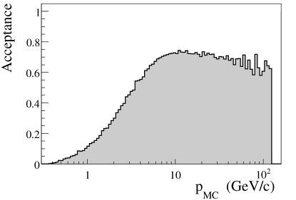
Figure 66: Tracking acceptance for hadrons as a function of the generated particle momentum.

Figure 67: Reconstruction efficiency as a function of the particle momentum.

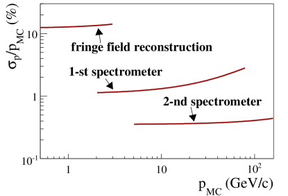
Figure 68: Relative track momentum resolution $\sigma_{p}/p$ versus $p$.

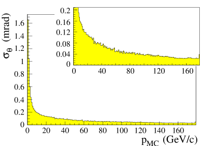
Figure 69: Resolution of the reconstructed particle emission angle at the interaction vertex as a function of the particle momentum.

10.8 RICH-1 performances

Figure 70 shows a two-dimensional histogram of the Cherenkov angles as measured with RICH-1, versus the particle momenta. The corresponding loci for pions, kaons and protons are clearly visible.

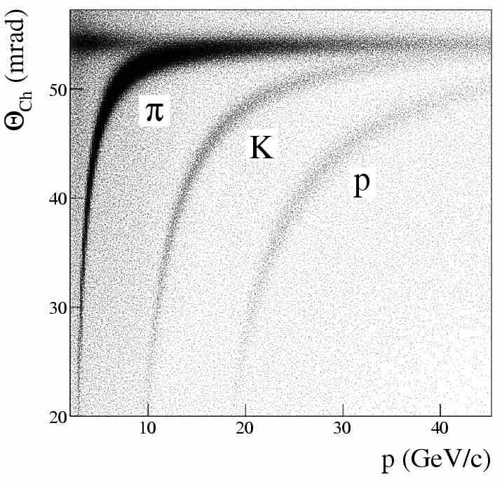
Figure 70: A two-dimensional histogram of the Cherenkov angles as measured with RICH-1 versus the particle momenta. The entries referring to particles identified as pions have been depressed by a factor of 3; those referring to particles identified as protons have been multiplied by a factor of 4.

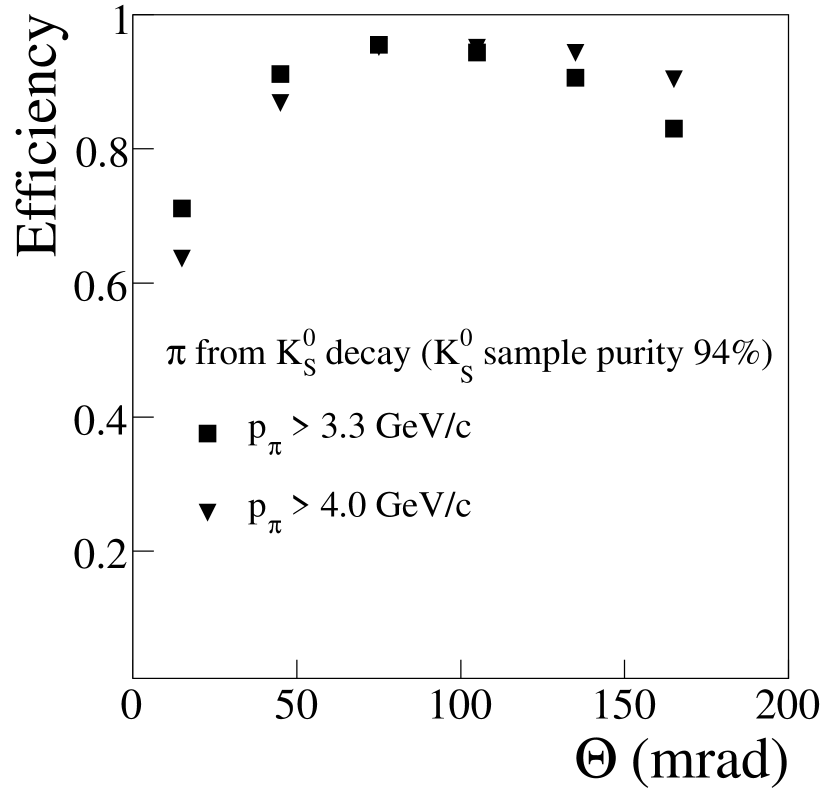
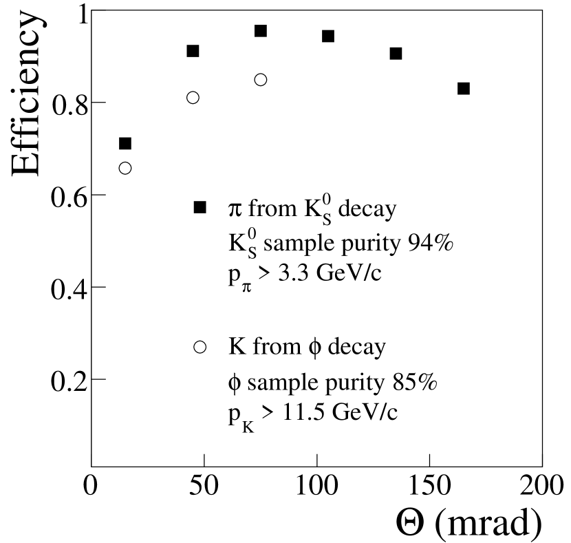
Figure 71: 2003 data, PID efficiency for pions from $K_{S}^{0}$ decay versus the particle polar angle, pion momentum $p>3.3\,\GeV/c$ (squares); left: comparison with PID efficiency for pions with momentum $p>4\,\GeV/c$ (triangles); right: comparison with PID efficiency for kaons from $\phi$ decays, kaon momentum $p>11.5\,\GeV/c$ (open circles).

Figure 71 (left) shows the PID efficiency for pions from $K_{S}^{0}$ decay versus the particle polar angle applying two different cuts to the particle momentum: $3.3\,\GeV/c$, corresponding to a mean value of 5 detected photoelectrons per particle and $4\,\GeV/c$, corresponding to a mean number of 8 detected photons. The $K_{S}^{0}$ sample has a purity of 94%. The efficiency is plotted versus the particle polar angle because different angles correspond to different regions of the photon detectors. For particles scattered at small polar angles, the signal to noise ratio is less favourable due to the overlap with the images generated by the huge beam halo of the SPS muon beam. Moreover, the presence of the beam pipe inside the RICH vessel and a corresponding hole in the mirror wall reduces the number of detectable photons for these particles. Particles scattered at large polar angle have, on average, low momentum.

Comparing PID efficiency for particles selected with different momentum cuts, it is shown that the slightly lower efficiency at large polar angles is related to samples with lower mean momentum value, thus with lower number of detected Cherenkov photons. For example, for the pions contributing to the point at largest polar angles, the mean value of the momentum distribution is as low as $4.3\,\GeV/c$ .

Figure 71 (right) presents the PID efficiency for kaons from $\phi$ decay versus the particle polar angle. Momenta larger than $11.5\,\GeV/c$, corresponding to a mean value of 5 detectable photoelectrons, were selected. The $\phi$ sample has a purity of 85%. The kinematic range explored is limited due to the phase space spanned by the diffractive $\phi$ production. The apparent reduced efficiency for K PID is compatible with the poorer purity of the $\phi$ sample.

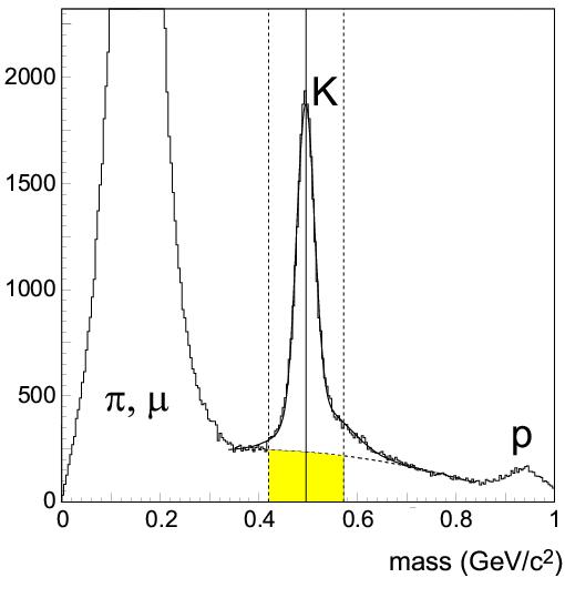
Figure 72: Reconstructed mass spectrum for particles with momenta $11.5\,\GeV/c$ and polar angle $>$ 25 mrad.

Figure 72 illustrates the achieved PID purity: the reconstructed mass spectrum, K region, for particles with momenta larger than $11.5\,\GeV/c$ and polar angle $>$ 25 mrad is shown. The signal S over background B ratio is 2.5 and the purity, defined as S / (S + B), is $>$ 0.7. The corresponding phase space region includes $\sim$75% of the kaons from $D^{0}$ and $\overline{D}^{0}$ decay, as selected applying standard COMPASS analysis cuts.

10.9 Energy reconstruction in the COMPASS calorimeters

In COMPASS, the energies of charged and neutral particles are reconstructed by means of two hadron calorimeters (HCAL1 and HCAL2, see Sec. 6.3.1 and 6.3.2) and one electromagnetic calorimeter (ECAL2, see Sec. 6.3.3). The energies and positions of the calorimeter showers are reconstructed by a dedicated software package, common to both types of calorimeters. The shower parameters are estimated from the energy deposited in clusters of neighbouring cells, assuming a known parameterization of the shower profile.

During the first step of the shower reconstruction, the local maxima are approximately identified by selecting the cells with an energy deposit above a predefined threshold. At this stage, two showers are not separated if the local maxima are located at nearby cells.

The energy and position of the cell corresponding to the local maximum are used as initial parameters for the shower reconstruction. The remaining part of the shower is searched in a region of $3\times 3$ or $5\times 5$ cells surrounding the local maxima. The region size depends on the estimated shower energy; for higher energies a larger region is selected. Although a local maximum can be attributed to one shower only, the energy deposited in the surrounding cells can be shared between two or more showers. Therefore, the initial values of energy and position for the shower are used to estimate the amount of energy deposited in the cells surrounding the local maximum. This procedure is repeated for all local maxima; the relative contribution of each shower to the shared cells is thus computed.

Once the amount of energy deposited in each cell by the expected showers is computed, a fitting procedure is applied to calculate the exact parameters (energy and position). The energy is simply calculated from the sum of cell energies, corrected for the shower leaks outside the calorimeter and for the shower overlaps. For the determination of the coordinate parameters, the inverse one-dimensional cumulative shower profile function [115] is used. In this approach, the theoretical two-dimensional shower surface is projected onto two planes, perpendicular to the calorimeter surface, one directed horizontally and one vertically. The projection of the shower surface is symmetric with respect to the shower axis, and the two boundaries are parameterized with analytical functions, the actual parameters of which are optimised for the hadron and electromagnetic cases. The position of the shower axis which gives the best fit to the energy distribution in the cells attributed to the shower determines the X and Y coordinates, depending on the projection surface.

A good estimation of the overall ECAL2 performances is given by the mass resolution for reconstructed $\eta\to\gamma\gamma$ decays. To estimate the width of the $\eta$ mass peak and minimise the combinatorial background, only events with exactly two clusters originating from neutral particles have been selected. The invariant mass is then calculated under the assumption that the two clusters were produced by two photons emitted from the reconstructed primary interaction vertex. The resulting mass distribution is shown in Fig. 73. The fit of the mass peak with a Gaussian function and a polynomial background gives a relative resolution of 4.6%, quite close to the theoretical limit of about 4% given by the intrinsic energy resolution of the calorimeter elements.

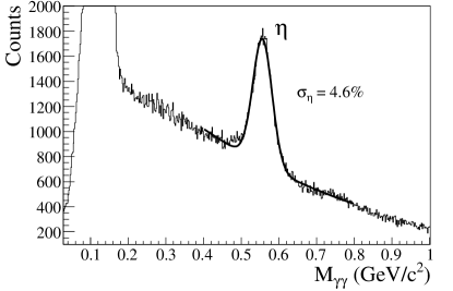
Figure 73: Invariant mass distribution in the hypothesis of $2\gamma$ neutral decays. The $\eta$ mass is determined from the gamma energy reconstructed in the electromagnetic calorimeter ECAL2, in the hypothesis that the photons originated from the primary interaction vertex.

11 Spectrometer upgrade

The COMPASS setup employed during the data taking periods in 2002, 2003 and 2004, and described in the previous sections, is not as complete as the one foreseen in the original design of the COMPASS spectrometer. Part of the components have been staged. For the data taking from 2006 on, an important upgrade of the COMPASS apparatus is implemented. It concerns the polarised target (see Sec. 11.1), the large area trackers of the LAS (see Sec. 11.2), the RICH-1 detector (see Sec. 11.3), the electromagnetic calorimeter ECAL1 (see Sec. 11.4), and the new tracker and preshower station located downstream of RICH-1 (see Sec. 11.5).

11.1 Polarised target

The original design of the COMPASS spectrometer included a large-aperture superconducting solenoid magnet, which maintains the polarisation of the target. The solenoid has been designed to match the required $\pm 180\,\mrad$ acceptance for the most downstream edge of the polarised target (see Sec. 4.1 for a description of the polarised target), while providing a homogeneity at least as good as the magnet used until 2004 in COMPASS, despite a volume five times larger.

The solenoid was delivered to the collaboration by Oxford Danfysik [116] at the end of 2004. Extensive tests were performed in order to fully characterise the intrinsic performances of the magnet. The relative intrinsic field uniformity was tuned to within $\pm 3\EE{-5}$ over the useful volume of the target cells ($130\,\cm$ total length, $3\,\cm$ diameter). A fully automated control system for the handling of the cryogenics and a fast safety system designed to trigger the heaters in case of a quench were implemented. A specific procedure involving the heaters on the shim coils had to be worked out in order to accommodate for a short circuit in one of the shims. After installing the magnet in its final position in the COMPASS hall, new optimisations of the shim coil currents were performed in order to account for the presence of the large SM1 dipole magnet yoke. A final relative field uniformity of $\pm 4\EE{-5}$ was achieved, valid for operation at both field orientations. Field profiles have also been measured in the region between the solenoid and SM1, providing additional input for the tracking software. As for the magnet used until 2004, a transverse field is required for field rotations and for measurements with transverse orientation of the target polarisation. A dipole coil provides such a transverse field of $0.6\,\T$.

The polarised target configuration used until 2004 consisted of two identical cells with opposite polarisation (see Sec. 4.1). The variation of the spectrometer acceptance for reaction products originating from the two cells is a source of false asymmetry, largely removed by reversing the cell polarisation every eight hours. A new target system was built for the new solenoid. It consists of three target cells and a redesigned microwave cavity adapted to the enlarged acceptance. In this new configuration, the central cell is twice longer than the two external cells and its target material is polarised in opposite direction to the external ones. Simulations show that such a configuration leads to a further reduction - by an order of magnitude - of the false asymmetry.

11.2 Large drift chamber and straw tubes

The two tracker telescopes of the LAS, located upstream and downstream of the SM1 analysing magnet, have to match the enlarged acceptance made possible by the availability of the COMPASS solenoid: $\pm 180\,\mrad$ in the horizontal and vertical projections between the polarised target and SM1 and $\pm 250\,\mrad$ in the horizontal projection between SM1 and RICH-1. Upstream of SM1, the existing tracker telescope is completed with an additional medium size drift chamber positioned immediately behind the first Micromegas station. Downstream of SM1 only one out of the three stations of the corresponding tracking telescope (see Sec. 5.3) has a transverse surface big enough to cover the enlarged angular acceptance. The two drift chambers are replaced by a new large drift chamber and by a second straw tube station, identical to the ones described in Sec. 5.3.2.

The new drift chamber has a design derived from trackers DC1, DC2 and DC3, already in operation in the COMPASS spectrometer (see Sec. 5.3.1). The active surface is enlarged to $248\times 208\,\cm^{2}$, compared to $180\times 127\,\cm^{2}$ for DC1–3. The chamber has eight active wire planes for the measurement of four coordinates (horizontal wires, vertical wires and wires inclined at $\pm 10$ degrees with respect to the vertical axis). The drift cells have a pitch of $8\,\mm$ and a gap of $8\,\mm$. The central dead zone has a diameter of $30\,\cm$. The total material budget of the chamber is $0.32\%$ of a radiation length. The readout system is identical to the one in use for DC1-3 chambers, namely ASD8 front-end chips coupled to F1-TDCs. Performances (efficiency, resolution) are expected to be identical to the ones obtained with stations DC1-3.

11.3 RICH-1

The overall RICH-1 upgrade project aims at a significant increase of the RICH performances in the years to come. It was designed to improve two important limitations of the RICH-1 detector. The first limitation comes from the large dispersed halo that generates high pad occupancies and deteriorates the signal-to-noise ratio (see 6.1.5), particularly in the central region. The halo also increases the probability for electrical instabilities of the photon detectors. The second limitation is due to the large dead time imposed by the architecture of the GASSIPLEX front-end chip (see Sec. 6.1.4).

In order to minimise the overall cost of the project, two complementary technologies have been chosen. In the most sensitive central region both the photon detectors and the readout system are replaced with a new photon detection system based on Multi-Anode Photo-Multiplier Tubes (MAPMT). In the peripheral region the existing photon detectors are kept, but their associated electronics is replaced with a new, much faster readout system based on the APV25 chip.

11.3.1 RICH-1 upgrade in the central region

The central part of the RICH-1 detector is instrumented with a system based on MAPMTs for fast photon detection. The time resolution, of a few ns, allows an efficient rejection of the high background due to uncorrelated events. Each MAPMT is coupled to a telescope formed by a field lens and a concentrator lens. These new detectors replace the four central photocathodes of the CsI MWPCs, corresponding to $25\%$ of the total active surface.

The approach to detect photons in RICH counters with MAPMTs and lenses is not new (HERA-B [117], studies for LHCb [118, 119]). In our design, two new elements are introduced: the detection of visible and UV photons and a largely increased ratio of the collection surface to the photocathode one. We extend the detected range of the Cherenkov light spectrum to the UV domain (down to $\sim 200\,\nm$) by using UV extended MAPMTs and fused silica lenses. We have selected the R7600-03-M16 MAPMT developed by Hamamatsu [32], characterised by a bialkali photocathode with $18\times 18\,\mm^{2}$ active surface, 16 pixels, 70% collection efficiency of photoelectrons and a UV extended glass entrance window extending the sensitive range down to $200\,\nm$. The effective pixel size of a MAPMT coupled to the lens telescope is 12$\times$12 mm². The resulting ratio of the entrance lens surface to the MAPMT photocathode surface has a value of about 7, thus reducing the number of MAPMTs and keeping the system at affordable cost.

The lens telescope has been designed in order to satisfy several important requirements. The image distortion has to be minimised, keeping the telescope length around $10\,\cm$, in spite of the large image demagnification and the large angular acceptance. Simulations show that only about $10\%$ of the photons are not detected in the corresponding MAPMT pixel, but in a nearby one. The telescope must have a large angular acceptance; the value achieved is about $\pm 165\,\mrad$, resulting in an estimated ring loss below $5\%$. The dead zone should be as small as possible; an accurate mechanical design assures only $2\%$ dead zone between field lenses.

The MAPMTs are read with a MAD4 amplifier-discriminator [56], housed on small front-end boards mounted directly onto the resistive divider boards. Power and thresholds are distributed via deck boards, while digital boards housing F1-TDC chips are directly coupled to the deck boards; the arrangement is without cables, thus very compact and reliable. The readout architecture is similar to that already successfully implemented in COMPASS for the Micromegas and DC detectors (see Sec. 8.3.3), and also used for the Rich wall detector . The photon detection principle has been validated in two test beam measurements at the CERN PS beam line T11 in summer 2003 and 2004 [120]. The MAPMTs have been studied and characterised for single photoelectron detection in the laboratory [121, 122]. Comparing Monte Carlo studies and test results, it has been shown that single photoelectrons collected by the MAPMT dynode system are detected with full efficiency. The long plateau of the threshold curves clearly indicates that noise and crosstalk can be efficiently rejected without photoelectron losses. At high rate, the MAPMT efficiency shows no losses up to single photoelectron rates of $5\,\MHz$ per pixel, while the front-end chip is limited to about $1\,\MHz$. A new version of the chip overcoming this limitation, C-MAD, is being developed and will be used in 2008 and beyond.

The new detection system collects a number of detected photons per ring that is a factor of 4 larger than the previous one; at saturation, and far from the central region affected by dead zones, this results in about 60 photons per ring. Due to the enlarged pixel size, the resolution on the measured Cherenkov angle from single photons is worsened by about a factor 1.5. This reduction is largely compensated by the increased number of detected photons. The angular resolution also benefits from the negligible uncorrelated background level. The expected resolution for a whole ring at saturation, and far from the central region is about $0.3\,\mrad$ (presently $0.45\,\mrad$). The improved resolution makes the $\pi$/K separation at $2.5\,\sigma$ possible up to at least $50\,\GeV/c$, to be compared with the present limit of $43\,\GeV/c$. Finally, the increased number of detected photons will lower the effective RICH thresholds; the new thresholds nearly coincide with the physical thresholds of the Cherenkov effect.

11.3.2 RICH-1 upgrade in the peripheral region

The existing system of MWPC with CsI photocathodes continues to equip the peripheral 75% of the active area of the RICH-1 detector. The readout system will be replaced by a new analogue sampling readout based on the APV25 chip [123], already employed to read COMPASS silicon (see Sec. 5.1.2) and GEM detectors (see Sec. 5.2.2). The time information obtained from the new system allows us to reduce the effective time gate of the RICH readout from presently $\approx 3.5\,\mus$ to less than $400\,\ns$, leading to a large suppression of the uncorrelated background. In addition, the system significantly reduces the readout dead time, making it similar to the rest of the experiment, i.e. 5% at $50\,\kHz$ trigger rate. Multiplexing 128 detector channels onto a single output channel also makes this solution very cost-effective.

The APV25 chip, although originally designed for silicon microstrip detectors, is used here for the first time to read “slow” signals from a MWPC, maintaining a signal-to-noise ratio of about 9. This is made possible by the fact that the time constants of the preamplifier and shaper stages of the chip can be increased from the standard value of $50\,\ns$ up to $500\,\ns$ by varying bias currents through feedback transistors. The sampling of the input signals is still performed at $40\,\MHz$, as for the silicon and GEM detectors; the three samples transferred per incoming trigger, however, are separated in time by $150\,\ns$ instead of $25\,\ns$ in order to cover the rising edge of the MWPC signal. The multiplexed information from each APV25 chip is digitised using a pipelined ADC, similar to the one described for the silicon and GEM detectors in Sec. 8.3.1. To allow a precise tuning of thresholds and efficient zero suppression, necessary due to the typical Polya amplitude distribution for single photon events, which has an approximately exponential shape at low gain, 12-bit ADCs are used for the RICH, in contrast to 10-bit ADCs for silicon and GEM detectors. The sampling rate of the ADCs is increased from $20\,\MHz$ to $40\,\MHz$ in order to keep the dead time at the expected value.

To match the configuration of the RICH-1 CsI photon detector, four APV25 chips are mounted on one front-end card, each APV25 reading 108 RICH pads. For optimum noise performance and reliability, four front-end cards are then directly connected to one ADC card, digitising 16 APV25 chips and distributing the trigger and control signals to the front-end cards. Two Virtex-4 FPGAs perform online common mode noise correction and zero suppression.

A full test of the proposed readout system was performed in nominal muon beam conditions in the central region of RICH-1 in 2004, with half the area of one photon detector equipped with APV25 chips and 5184 channels read out by 10-bit ADCs. For the optimal APV25 settings a signal-to-noise ratio very similar to the original GASSIPLEX-based readout was obtained, the higher ballistic deficit of the APV25 readout being fully compensated by a lower average noise figure. As a consequence, the detection efficiency for single photoelectrons was found to be very close to that obtained with the GASSIPLEX. The signal-to-background ratio, however, is strongly increased by the new readout due to its increased time resolution. A gain by a factor of 5-6 was measured in the central region, where pile-up due to the muon beam halo is most significant.

11.4 Electromagnetic calorimeter

An electromagnetic calorimeter (ECAL1), with overall dimensions of $4.00\times 2.91\,\m^{2}$ is assembled and positioned upstream of the HCAL1 hadronic calorimeter. The ECAL1 calorimeter covers the angular acceptance of $\pm 180\,\mrad$ made possible by the use of the new solenoid magnet. It allows measurements of reaction channels with the production of low energy prompt photons and/or neutral pions.

The ECAL1 calorimeter is formed by blocks of three different sizes. The most central region is equipped with 576 blocks of $38.2\times 38.2\,\mm^{2}$, originating from the GAMS calorimeter [82]. In the intermediate region 580 blocks of $75\times 75\,\mm^{2}$ from a calorimeter built for the WA89 experiment at CERN [124] are used. The most external region is filled with 320 blocks from the OLGA calorimeter [125] with dimensions of $143\times 143\,\mm^{2}$. The signal amplitude from all the calorimeter blocks are read by fast sampling SADCs, identical to the ones described in Sec. 8.3.2.

11.5 Rich wall

A new large-size (4.86 $\times$ 4.22 m²) tracking station (Rich wall), is positioned downstream of RICH-1, directly in front of the ECAL1 electromagnetic calorimeter. It consists of eight layers of MDT modules (see Sec. 6.2.1, Fig. 43) that have the same design as MW1, apart from a thinner Al profile ($0.45\,\mm$ instead of $0.6\,\mm$). Mechanically, the Rich wall detector is similar to one station of MW1 (see Fig. 44), with a converter inserted in front of each of the four pairs of layers. Each converter is a sandwich of three plates (steel/lead/steel), resulting in a total converter thickness of about 3 radiation lengths. The Rich wall detector provides up to four coordinate points per track in two projections, $X$ and $Y$. The required coordinate accuracy (of about $0.8\,\mm$ r.m.s. per plane) is obtained by reading out the MDT modules in drift mode. Ageing tests performed with an Ar/CO₂ (70/30) gas mixture have shown no degradation effects up to $1\,\C/\cm$. The beam-induced MDT charge, integrated over the lifetime of the COMPASS experiment, is comparable to that value; therefore no performance degradation is expected for the duration of the experiment.

The Rich wall tracker station performs a twofold function in the COMPASS spectrometer. First, it measures the particle trajectories downstream of the RICH, thus allowing a better reconstruction of the particle trajectories in the RICH volume. Second, it acts as preshower for the ECAL1 electromagnetic calorimeter, thus improving the spatial resolution of the calorimeter itself.

12 Summary and outlook

An overview of the COMPASS experimental setup, as used in the 2004 run, was given in this article. The setup was designed with the purpose of detecting one or more outgoing hadrons in coincidence with the scattered beam particle, in a large momentum range, for large angular acceptances and at high incident flows. In order to fulfil these requirements the outgoing particles are detected in a two-stage spectrometer, built around two large dipole magnets. The setup was built using various detector technologies, standard and novel ones. Charged particle tracks are measured using scintillation fibre hodoscopes, planes of high-precision silicon microstrips, large-size, high-resolution, minimal material budget GEM and Micromegas micropattern gas detectors, MWPCs, various sets of large-size drift chambers, straw drift tubes, planes of mini drift tubes and of stainless steel drift tubes. Particle identification is an important requirement for most of the COMPASS physics programme. It is performed making use of a large dimensions RICH detector, based on MWPCs with CsI photocathodes as photon detection technology, and tuned for momenta between $5$ and $43\,\GeV/c$, of an electromagnetic calorimeter, two hadron calorimeters and two muon filters. The trigger system makes use of scintillating counter hodoscopes and of the hadron calorimeter information. Several custom-made electronics devices such as the SFE16 front-end, F1-TDC and trigger matrix chips, the CATCH, GeSiCA and SADC readout modules and several specific front-end boards have been developed in order to match the COMPASS specifications, in particular the capability to stand high beam and trigger rates and the request of minimising the dead time generated by the data acquisition system.

Most of the equipments, designed for use in both muon and hadron experimental programmes, were commissioned between 2001 and 2002; some additional detector planes have been added for the 2003 and for the 2004 data taking. Up to 2004, the apparatus has been optimised and successfully operated mostly with a muon beam. A first pilot run with a hadron beam was also carried out.

All the COMPASS detectors, targets, control and monitoring packages, reconstruction and analysis software were described. Emphasis was put on their general features and on the characteristics obtained in nominal muon beam conditions. Performances of the whole setup were summarised.

The upgrade, as put in operation for the data taking phase starting in 2006, was also described. With this setup fully operational, COMPASS can complete the study of hadron structure using leptonic probes. The physics programme with hadron beams has been only marginally addressed until now, with the measurement of the pion polarisabilities during the 2004 pilot hadron run, and is scheduled from 2007 on. It comprises a variety of measurements, including central production of light mesons and production of heavy flavours, which require further upgrades of the apparatus in addition to the ones completed for the 2006 run. Thin targets surrounded by radiation-hard high-precision silicon trackers are needed to achieve the required mass resolutions and to separate the production and decay vertices of charmed hadrons. Precise tracking close to the beam in the spectrometer requires the use of light detectors with little material budget in order to minimise secondary interactions outside the target. Radiation-hard electromagnetic calorimeter modules are foreseen to cope with the required beam intensities. Additional trigger devices will be necessary to select the desired final states and kinematical regions.

In summary, the COMPASS setup is fully operational and is being used for a broad nucleon structure and spectroscopy programme. The upgrade completed in 2006 insures data taking with further improved performances in the forthcoming years.

References

- [1] COMPASS Collaboration, G. Baum, et al., Compass: A proposal for a COmmon Muon and Proton Apparatus for Structure and Spectroscopy, CERN/SPSLC 96-14, SPSC/P 297 (March 1996).
- [2] S. D. Bass, Rev. Mod. Phys. 77 (2005) 1257.
- [3] F. Bradamante, et al. (Eds.), Workshop on future physics @ COMPASS, 2004, Yellow Report CERN-2004-011.
- [4] COMPASS Collaboration, E. S. Ageev, et al., Phys. Lett. B 612 (2005) 154.
- [5] COMPASS Collaboration, V. Y. Alexakhin, et al., Phys. Rev. Lett. 94 (2005) 202002.
- [6] COMPASS Collaboration, E. S. Ageev, et al., Eur. Phys. J. C41 (2005) 469.
- [7] COMPASS Collaboration, E. S. Ageev, et al., Phys. Lett. B 633 (2006) 25.
- [8] K. Kurek, et al., Nucl. Instr. and Meth. A 485 (2002) 720.
- [9] SMC, D. Adams, et al., Phys. Rev. D 56 (1997) 5330.
- [10] N. Doble, et al., Nucl. Instr. and Meth. A 343 (1994) 351.
- [11] EMC, O. C. Allkofer, et al., Nucl. Instr. and Meth. 179 (1981) 445.
- [12] C. Bovet, et al., The CEDAR counters for particle identification in the SPS secondary beams, CERN Yellow Report, CERN 82-13 (1982).
- [13] A. Abragam, The Principles of Nuclear Magnetism, The Clarendon Press, Oxford, 1961.
- [14] J. Ball, Nucl. Instr. and Meth. A 526 (2004) 7.
- [15] S. Goertz, et al., Nucl. Instr. and Meth. A 356 (1995) 20.
- [16] S. Bültmann, et al., Nucl. Instr. and Meth. A 425 (1999) 23.
- [17] SMC, D. Adams, et al., Nucl. Instr. and Meth. A 437 (1999) 23.
- [18] A. Dael, et al., IEEE Trans. Mag. 28 (1992) 560.
- [19] J. Ball, et al., Nucl. Instr. and Meth. A 498 (2003) 101.
- [20] A. Meier, 6LiD für das Polarisierte Target des COMPASS-Experiments, Ph.D. thesis, Ruhr-Universität Bochum, Germany (2001).
- [21] S. Neliba, et al., Nucl. Instr. and Meth. A 526 (2004) 144.
- [22] K. Kondo, et al., Nucl. Instr. and Meth. A 526 (2004) 70.
- [23] F. Gautheron, et al., The COMPASS polarized target, in: SPIN 2004: proceedings of 16th International Spin Physics Symposium and Workshop on Polarized Electron Sources and Polarimeters, Trieste, Italy, 10-16 October 2004, 2005, p. 791.
- [24] J. Koivuniemi, et al., Polarization build up in COMPASS 6LiD target, in: SPIN 2004: proceedings of 16th International Spin Physics Symposium and Workshop on Polarized Electron Sources and Polarimeters, Trieste, Italy, 10-16 October 2004, 2005, p. 796.
- [25] J. Koivuniemi, et al., Nucl. Instr. and Meth. A 526 (2004) 100.
- [26] O. V. Lounasmaa, Experimental Principles and Methods Below 1 K, Academic Press, 1974.
- [27] F. Pobell, Matter and Methods at Low Temperatures, Springer-Verlag, 1996.
- [28] Y. M. Antipov, et al., Phys. Lett. B 121 (1983) 445.
- [29] J. Bisplinghoff, et al., Nucl. Instr. and Meth. A 490 (2002) 101.
- [30] S. Horikawa, et al., Nucl. Instr. and Meth. A 516 (2004) 34.
- [31] Kuraray Co. Ltd., Methacrylic Resin Division, Tokyo, 103-0027 Japan, http://www.kuraray.co.jp.
- [32] Hamamatsu Photonics K.K., 14-5 Shimokanzo, Toyooka village, Shizouka-ken, Japan, http://www.hamamatsu.com.
- [33] A. Gorin, Nucl. Instr. and Meth. A 452 (2000) 280.
- [34] I. Abt, et al., Nucl. Instr. and Meth. A 439 (2000) 2.
- [35] M. J. French, et al., Nucl. Instr. and Meth. A 466 (2001) 359.
- [36] H. Angerer, et al., Nucl. Instr. and Meth. A 512 (2003) 229.
- [37] V. Palmieri, et al., Nucl. Instr. and Meth. A 413 (1998) 475.
- [38] D. Thers, et al., Nucl. Instr. and Meth. A 469 (2001) 133.
- [39] F. Kunne, Nucl. Phys. A 721 (2003) 1087c.
- [40] C. Bernet, et al., Nucl. Instr. and Meth. A 536 (2005) 61.
- [41] E. Delagnes, et al., IEEE Trans. Nucl. Sci. 47 (2000) 1447.
- [42] F. Sauli, Nucl. Instr. and Meth. A 386 (1997) 531.
- [43] Kaneka Corporation, Pasadena, USA, http://www.kanekahightech.com.
- [44] M. C. Altunbas, et al., Nucl. Instr. and Meth. A 490 (2002) 177.
- [45] B. Ketzer, et al., IEEE Trans. Nucl. Sci. 48 (2001) 1065.
- [46] S. Bachmann, et al., Nucl. Instr. and Meth. A 479 (2002) 294, CERN-EP-2000-151.
- [47] B. Ketzer, et al., IEEE Trans. Nucl. Sci. 49 (2002) 2403, CERN-OPEN-2002-004.
- [48] G. Bencivenni, et al., Nucl. Instr. and Meth. A 488 (2002) 493.
- [49] M. Bozzo, et al., Design and construction of the triple-GEM detector for TOTEM, in: Proc. IEEE Nuclear Science Symposium, Rome, 2004.
- [50] B. Ketzer, et al., Nucl. Instr. and Meth. A 535 (2004) 314.
- [51] M. C. Altunbas, et al., Nucl. Instr. and Meth. A 515 (2003) 249.
- [52] DuPont, U.S.A., http://www.dupont.com.
- [53] F. M. Newcomer, et al., IEEE Trans. Nucl. Sci. 40 (1993) 630.
- [54] V. N. Bychkov, et al., Nucl. Instr. and Meth. A 556 (2006) 66.
- [55] K. Platzer, et al., IEEE Trans. Nucl. Sci. 52 (2005) 793.
- [56] F. Gonella, et al., The MAD, a full custom ASIC for the CMS barrel muon chambers front end electronics, CERN/LHCC 2001-034, 7th Workshop on Electronics for LHC Experiments, Stockholm, Sweden, 10-14 Sep 2001 (2001).
- [57] F. W. Brasse, et al., Construction of a large drift chamber and test measurements, Internal Report, DESY F21-76/02 (August 1976).
- [58] E. Albrecht, et al., Nucl. Instr. and Meth. A 553 (2005) 215, and references therein.
- [59] E. Albrecht, et al., Nucl. Instr. and Meth. A 502 (2003) 266.
- [60] E. Albrecht, et al., Nucl. Instr. and Meth. A 510 (2003) 262.
- [61] E. Albrecht, et al., Nucl. Instr. and Meth. A 502 (2003) 236.
- [62] E. Albrecht, et al., Nucl. Instr. and Meth. A 502 (2003) 112.
- [63] RD26 Collaboration, RD26 status report, CERN/DRDC 93-36 (1993).
- [64] RD26 Collaboration, RD26 status report, CERN/DRDC 94-49 (1994).
- [65] RD26 Collaboration, RD26 status report, CERN/DRDC 96-20 (1996).
- [66] ALICE Collaboration, Detector for high momentum PID, technical design report, CERN/LHCC 98-19 (August 1998).
- [67] E. Albrecht, et al., Nucl. Instr. and Meth. A 518 (2004) 586.
- [68] E. Albrecht, et al., Nucl. Instr. and Meth. A 504 (2003) 354.
- [69] J. C. Santiard, et al., GASSIPLEX: a low noise analog signal processor for read-out of gaseous detectors, presented at the 6th Pisa Meeting on Advanced Detectors, La Biodola, Isola d’Elba, Italy (1994).
- [70] E. Iarocci, Nucl. Instr. and Meth. 217 (1983) 30.
- [71] W. Busza, Nucl. Instr. and Meth. A 265 (1988) 210.
- [72] V. M. Abazov, et al., preprint JINR P13-2003-198 (submitted to PTE), Dubna (2003) .
- [73] V. M. Abazov, et al., preprint JINR P13-2004-155 (submitted to PTE), Dubna (2004) .
- [74] G. D. Alexeev, et al., Nucl. Instr. and Meth. A 462 (2001) 494.
- [75] G. D. Alexeev, et al., Nucl. Instr. and Meth. A 423 (1999) 157.
- [76] G. D. Alexeev, et al., Nucl. Instr. and Meth. A 473 (2001) 269.
- [77] G. D. Alexeev, et al., communication JINR E13-2005-37, Dubna (2005) .
- [78] C. Brown, et al., Nucl. Instr. and Meth. A 279 (1989) 331.
- [79] N. V. Vlasov, et al., Instruments and Experimental Techniques 49 (2006) 41.
- [80] F. Binon, et al., Nucl. Instr. and Meth. A 256 (1987) 444.
- [81] D. Alde, et al., Nucl. Phys. B 269 (1986) 485.
- [82] F. Binon, et al., Nucl. Instr. and Meth. A 248 (1986) 86.
- [83] M. Kobayashi, et al., Nucl. Instr. and Meth. A 345 (1994) 210.
- [84] F. Binon, et al., Nucl. Instr. and Meth. A 214 (1983) 269.
- [85] F. Binon, et al., CERN preprint CERN-EP/81-27 (1981).
- [86] C. Bernet, et al., Nucl. Instr. and Meth. A 550 (2005) 217.
- [87] H. C. van der Bij, et al., IEEE Trans. Nucl. Sci. 44 (1997) 398.
- [88] RD12 Collaboration, 1997 status report on the RD12 project, CERN/LHCC 97-29 (April 1997).
- [89] B. Grube, et al., Architecture of a common GEM and silicon readout for the COMPASS experiment, Proceedings of the 7th International Conference on Advanced Technology and Particle Physics (ICATPP-7), Como, Italy, World Scientific (2001).
- [90] H. Fischer, et al., Nucl. Instr. and Meth. A 461 (2001) 507.
- [91] ALICE DAQ and ECS user’s guide, ALICE-INT-2005-015 v.1.
- [92] J.-P. Baud, et al., CASTOR status and evolution, in: Computing in high energy and nuclear physics (CHEP03), La Jolla, CA, USA, 2003, arXiv:cs.oh/0303241.
- [93] ETM professional control GmbH, Eisenstadt, Austria, http://www.pvss.com.
- [94] CAEN, Viareggio (LU), Italy, http://www.caen.it.
- [95] iseg Spezialelektronik GmbH, 01454 Radeberg, Germany, http://www.iseg-hv.de/.
- [96] W-IE-NE-R Plein & Baus GmbH, Burscheid, Germany, http://www.wiener-us.com/index.htm.
- [97] B. Hallgren, et al., The embedded local monitor board (ELMB) in the LHC front-end I/O control system, in: Proc. 7th Workshop on Electronics for the LHC Experiments, Stockholm, 10-14 September 2001, CERN 2001-005, CERN/LHCC/2001-034, 2001, p. 325.
- [98] The OPC Foundation, http://www.opcfoundation.org/.
- [99] http://itcofe.web.cern.ch/itcofe/Projects/SLiC.
- [100] C. Gaspar, et al., Comput. Phys. Commun. 140 (2001) 102.
- [101] D. R. Myers, et al., The LHC experiments’ joint controls project, JCOP, in: Proc. 7th International Conference on Accelerator and Large Experimental Physics Control Systems, 1999, http://accelconf.web.cern.ch/AccelConf/ica99 /proceedings.html.
- [102] MySQL AB, 753 20 Uppsala, Sweden, http://www.mysql.com.
- [103] C. Bernet, Caractérisation des Micromégas et mesure de la polarisation des gluons sur COMPASS (in French), Ph.D. thesis, Université Paris 7 - Denis Diderot (2004).
- [104] R. Brun, et al., Nucl. Instr. and Meth. A 389 (1997) 81, http://root.cern.ch.
- [105] R. Frühwirth, Nucl. Instr. and Meth. A 262 (1987) 444.
- [106] E. J. Wolin, et al., Nucl. Instr. and Meth. A 329 (1993) 493.
- [107] V. Blobel, et al., A new method for the high-precision alignment of track detectors, in: Proc. PHYSTAT2002, 2002, hep-ex/0208021.
- [108] G. Baum, et al., Nucl. Instr. and Meth. A 502 (2003) 315.
- [109] T. Ypsilantis, et al., Nucl. Instr. and Meth. A 343 (1994) 30.
- [110] GEANT - detector description and simulation tool, CERN Program Library Long Writeup W5013, http://wwwasdoc.web.cern.ch/wwwasdoc /geant_html3/geantall.html.
- [111] G. Ingelman, et al., Comput. Phys. Commun. 101 (1997) 108.
- [112] G. Ingelman, et al., Comput. Phys. Commun. 101 (1997) 135.
- [113] T. Sjöstrand, et al., Comput. Phys. Commun. 135 (2001) 238.
- [114] I. Akushevich, et al., RADGEN 1.0. Monte Carlo Generator for Radiative Events in DIS on Polarized and Unpolarized Targets, hep-ph/9906408 (1999).
- [115] A. A. Lednev, Nucl. Instr. and Meth. A 366 (1995) 292.
- [116] Oxford Danfysik, Oxford, Oxfordshire, OX2 0ES, UK, http://www.oxford-danfysik.com.
- [117] J. Pyrlik, et al., Nucl. Instr. and Meth. A 446 (2000) 299.
- [118] LHCb Collaboration, LHCb technical design report, CERN/LHCC/2000-37 (2000).
- [119] E. Albrecht, et al., Nucl. Instr. and Meth. A 488 (2002) 110.
- [120] M. Alekseev, et al., Nucl. Instr. and Meth. A 553 (2005) 53.
- [121] P. Abbon, et al., Nucl. Instr. and Meth. A 567 (2006) 114.
- [122] P. Abbon, et al., Studies for a fast RICH, presented at the 9th ICATPP, International conference on advanced technology and particle physics, Villa Olmo, Italy, 2005.
- [123] P. Abbon, et al., Nucl. Instr. and Meth. A 567 (2006) 104.
- [124] W. Brückner, et al., Nucl. Instr. and Meth. A 313 (1992) 345.
- [125] NA 14 Collaboration, P. Astbury, et al., Phys. Lett. B 152 (1985) 419.